
An Efficient Approach for Predicting Resonant Response with the Utilization of the Time Transformation Method and the Harmonic Forced Response Method


Abstract
:1. Introduction
2. Investigation Methodology
2.1. Prediction of the Aerodynamic Excitation
2.2. Prediction of the Damping
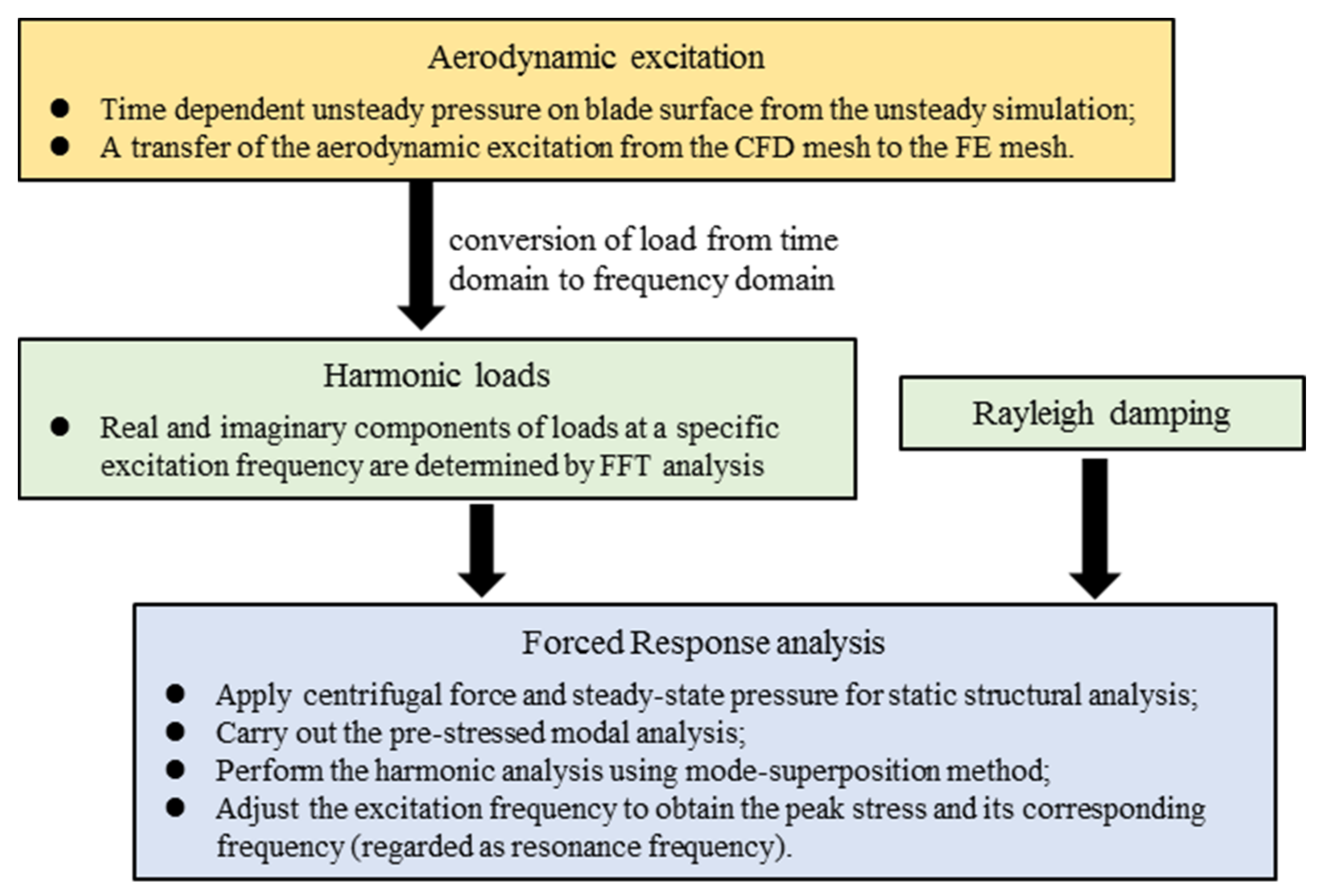
2.3. Prediction of the Vibration Response
- and are the amplitude and the phase angle of the loads;
- and are the real and imaginary parts of the loads;
- and are the amplitude and the phase angle of the displacements;
- and are the real and imaginary parts of the displacements.
3. Test Case
4. Results and Discussion
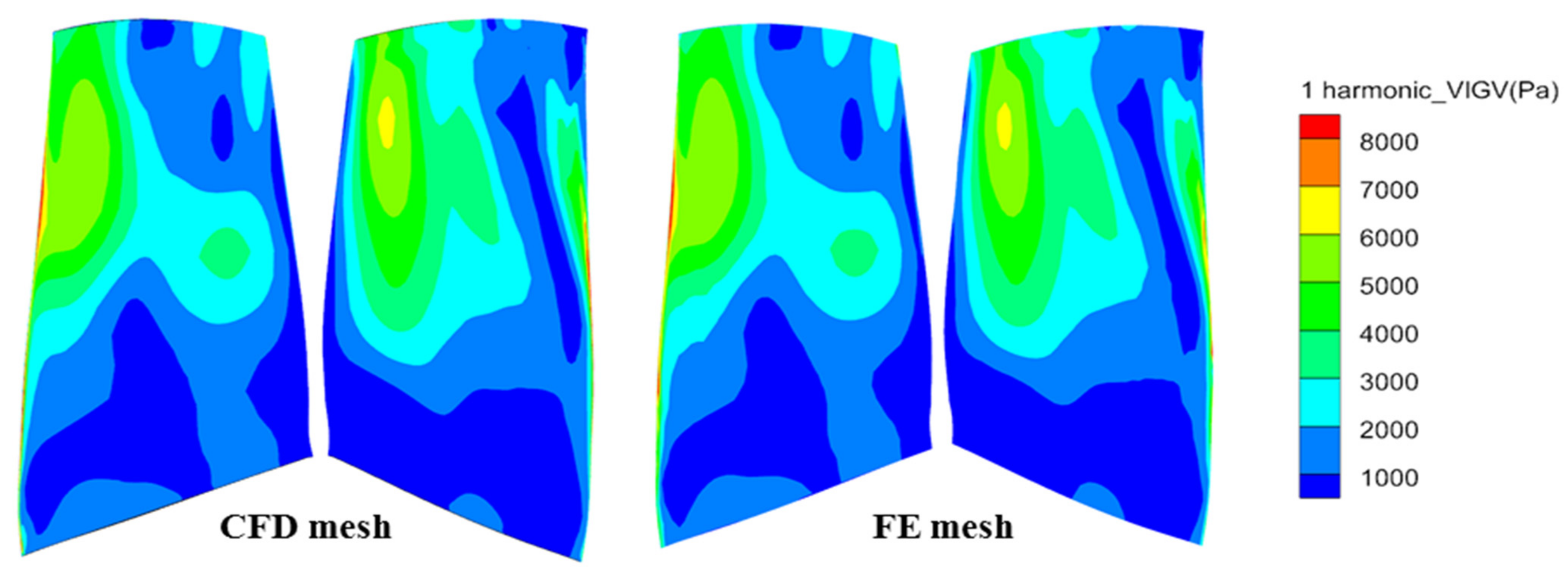
4.1. Aerodynamic Excitation
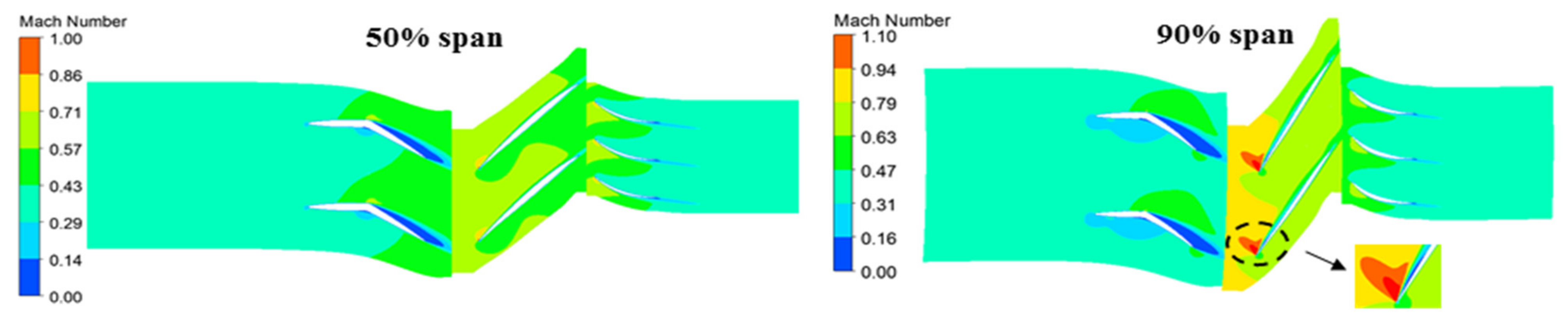
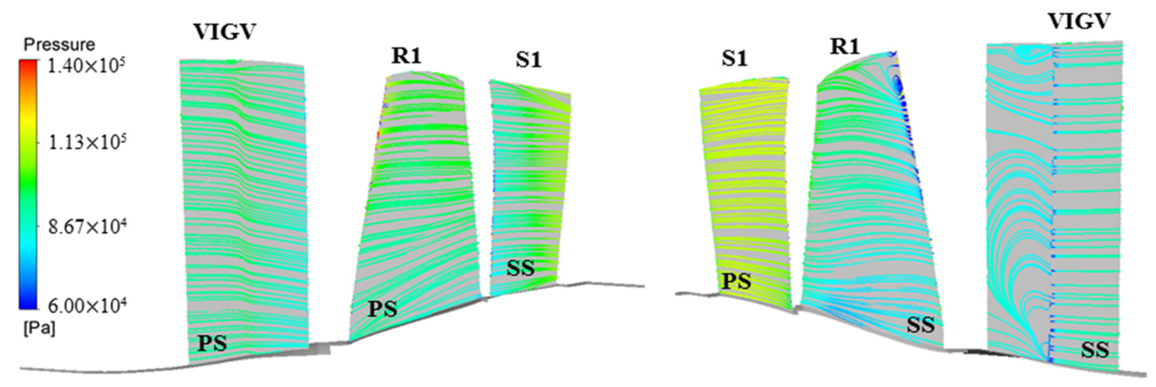
4.1.1. Steady Simulation
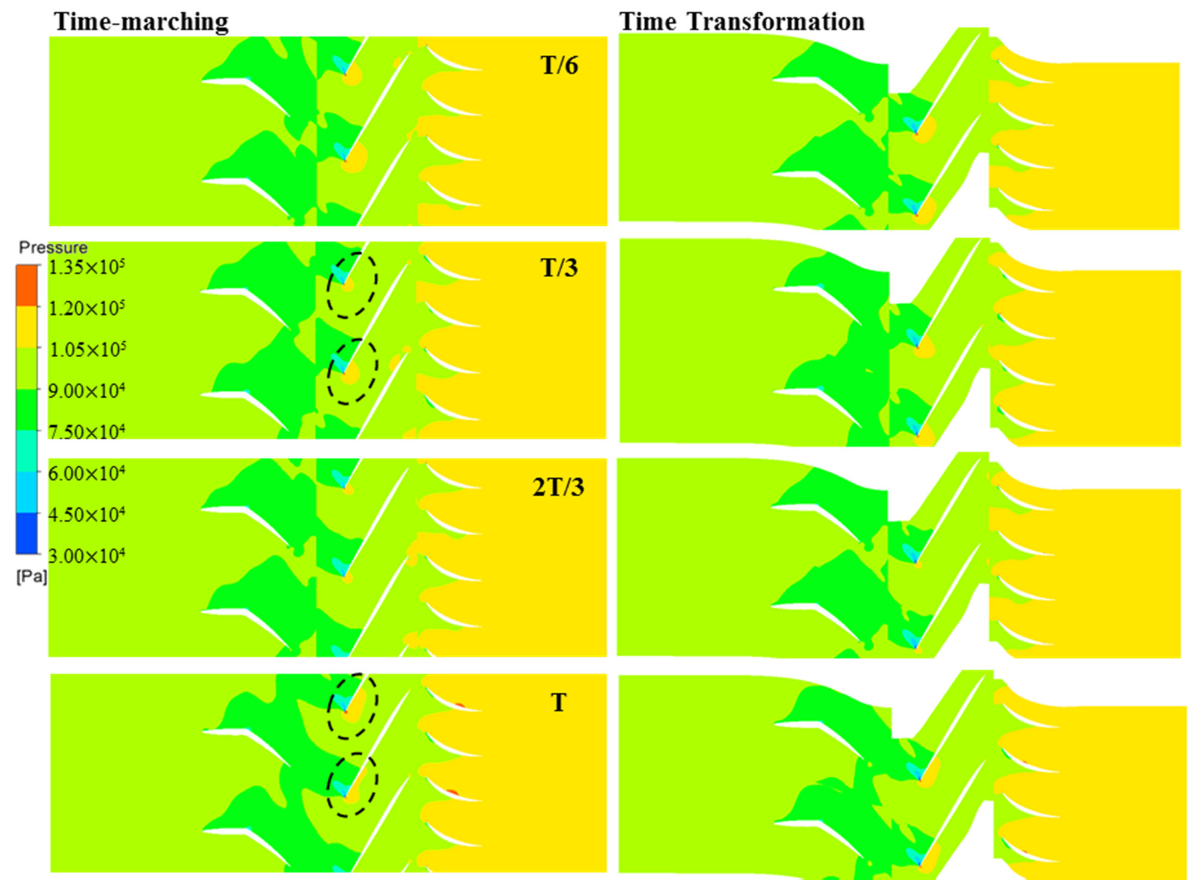
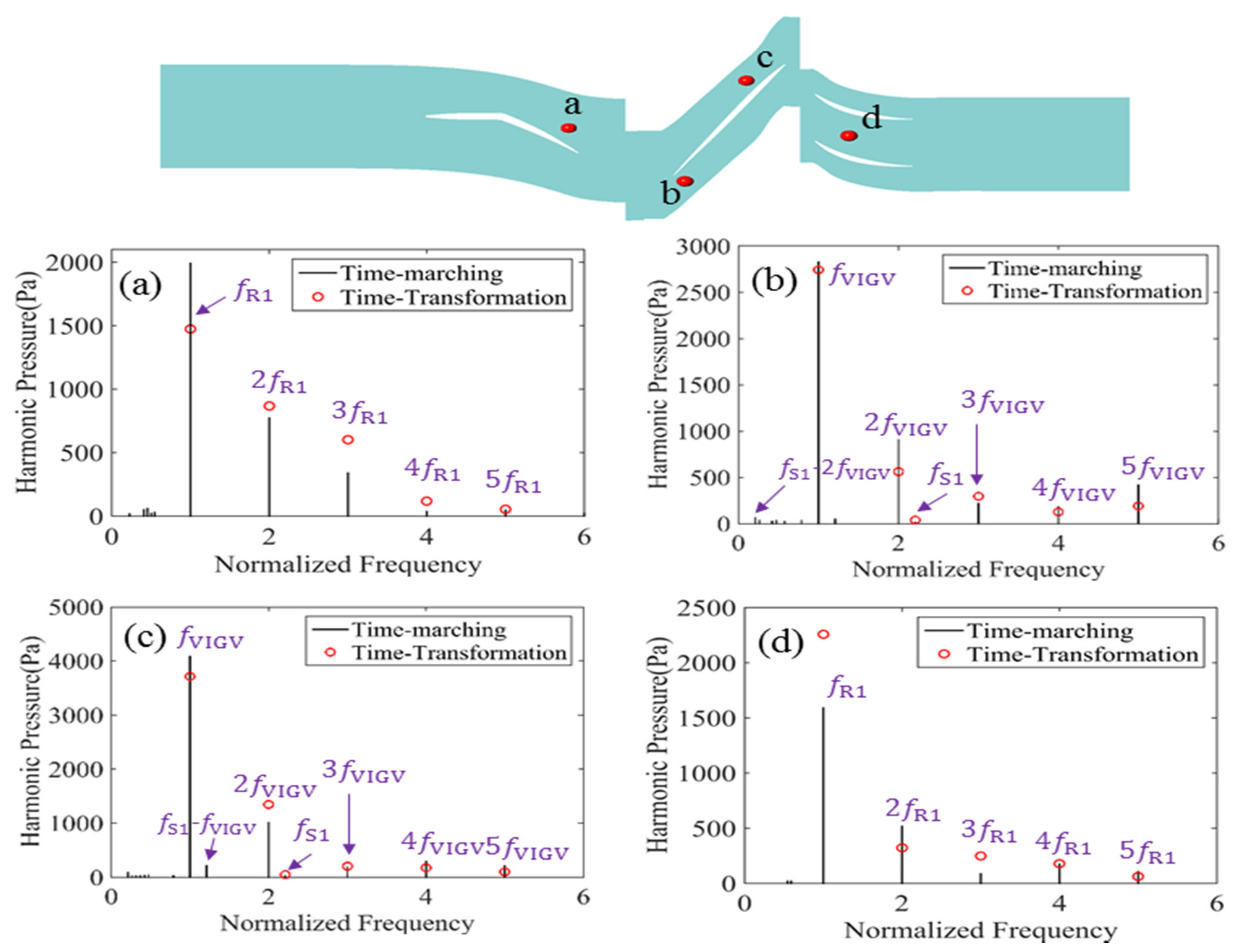
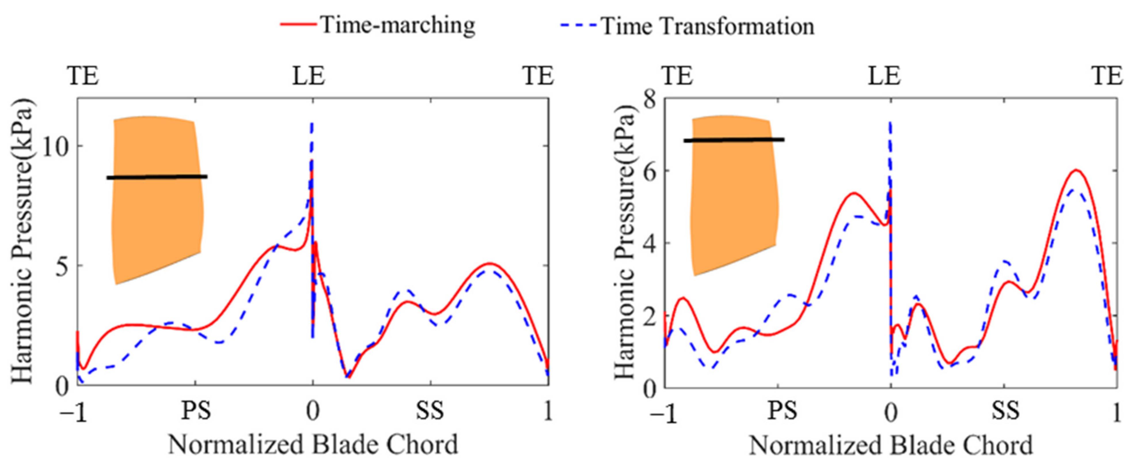
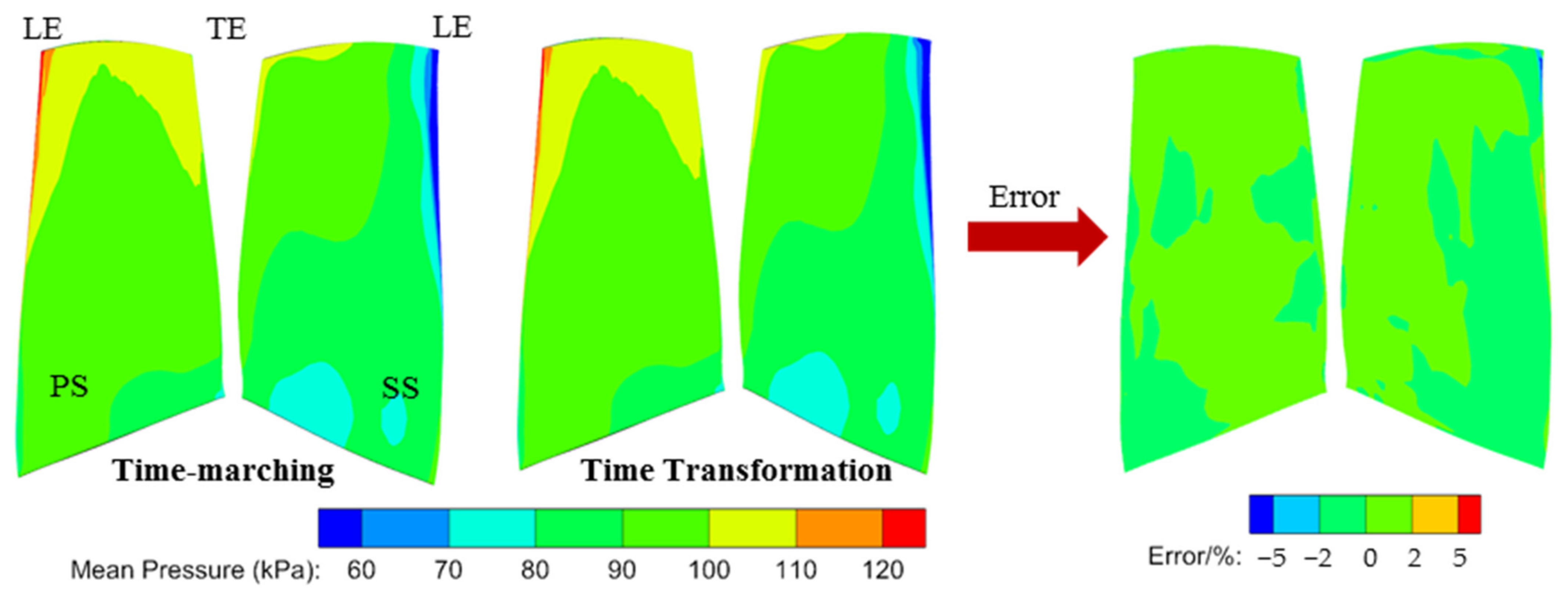
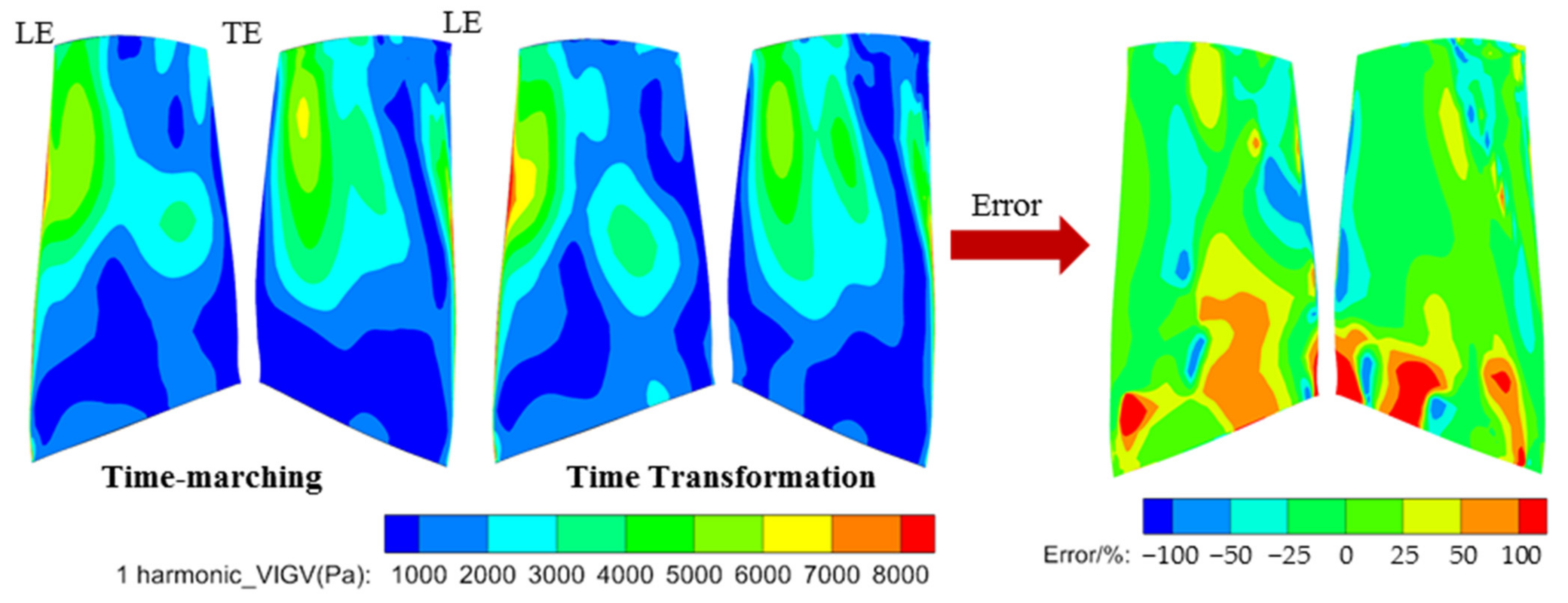
4.1.2. Unsteady Simulation
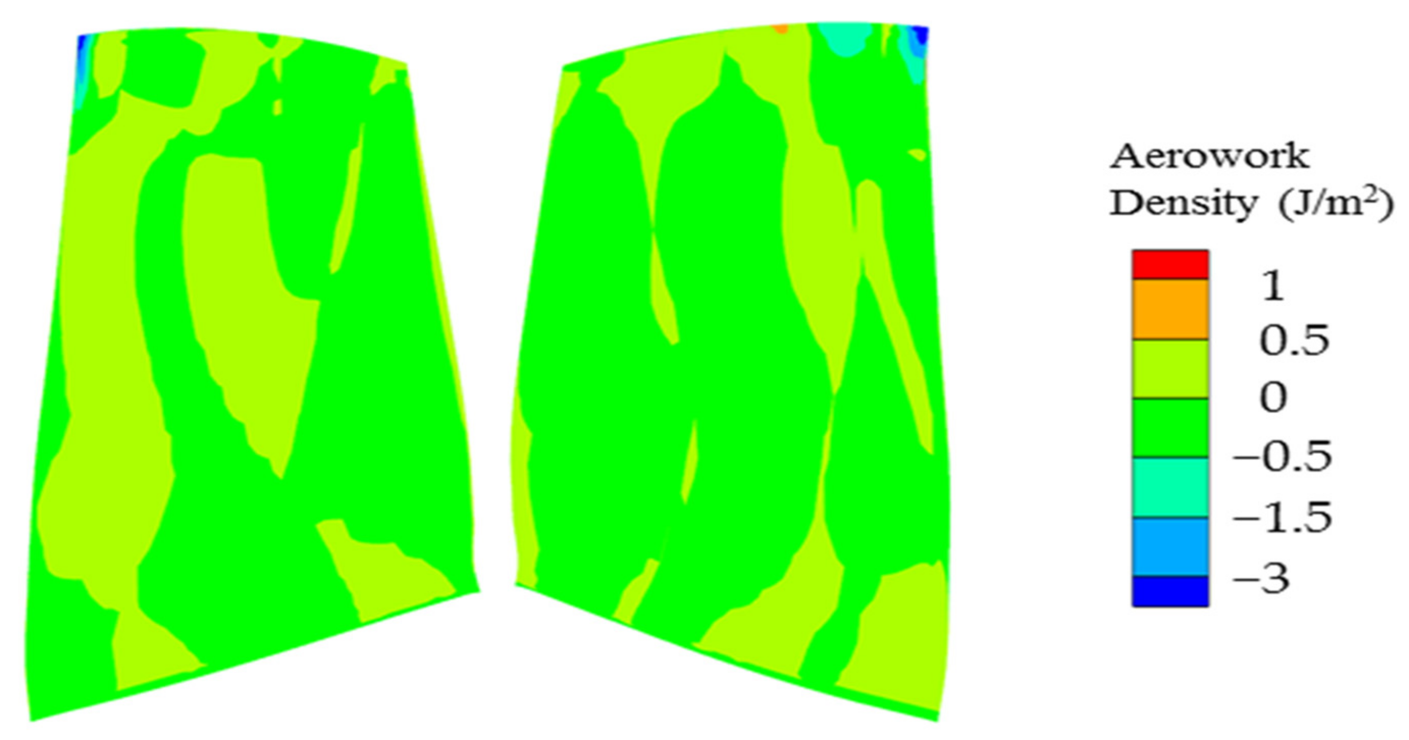
4.2. Aerodynamic Damping
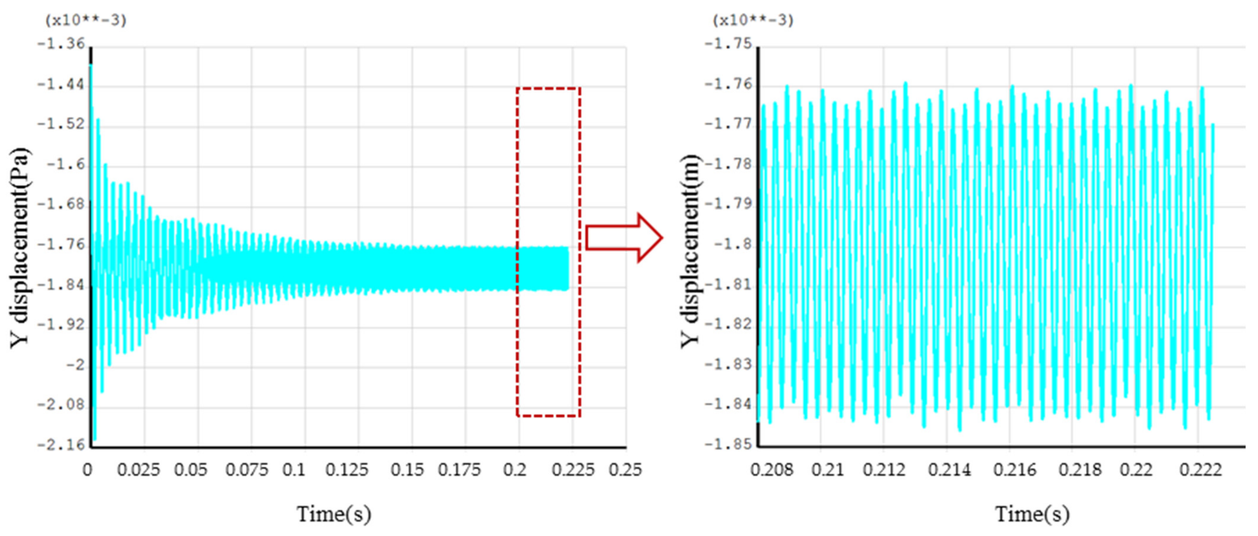
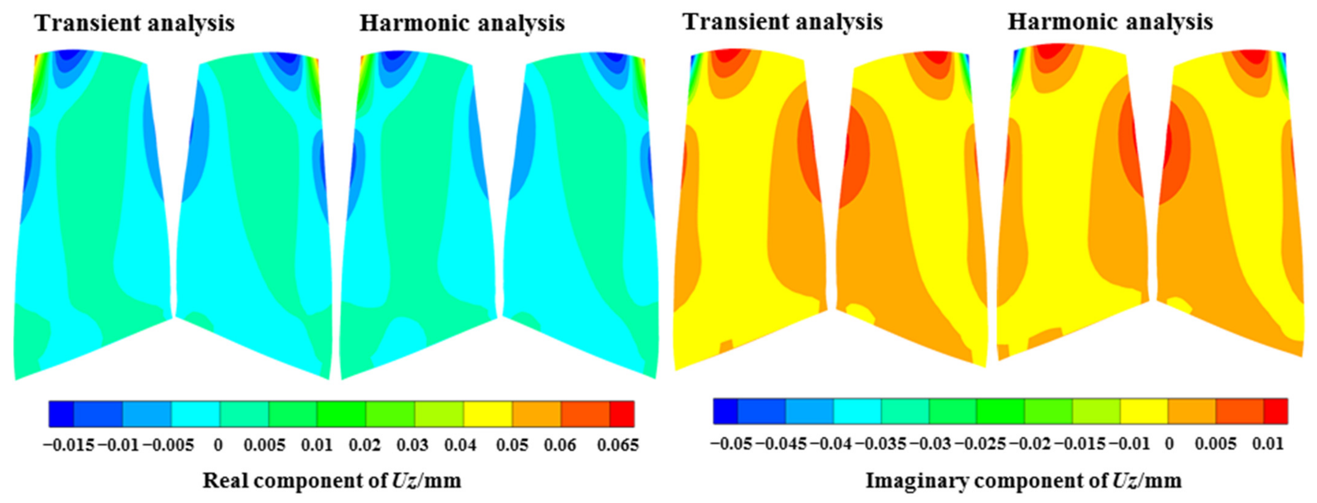
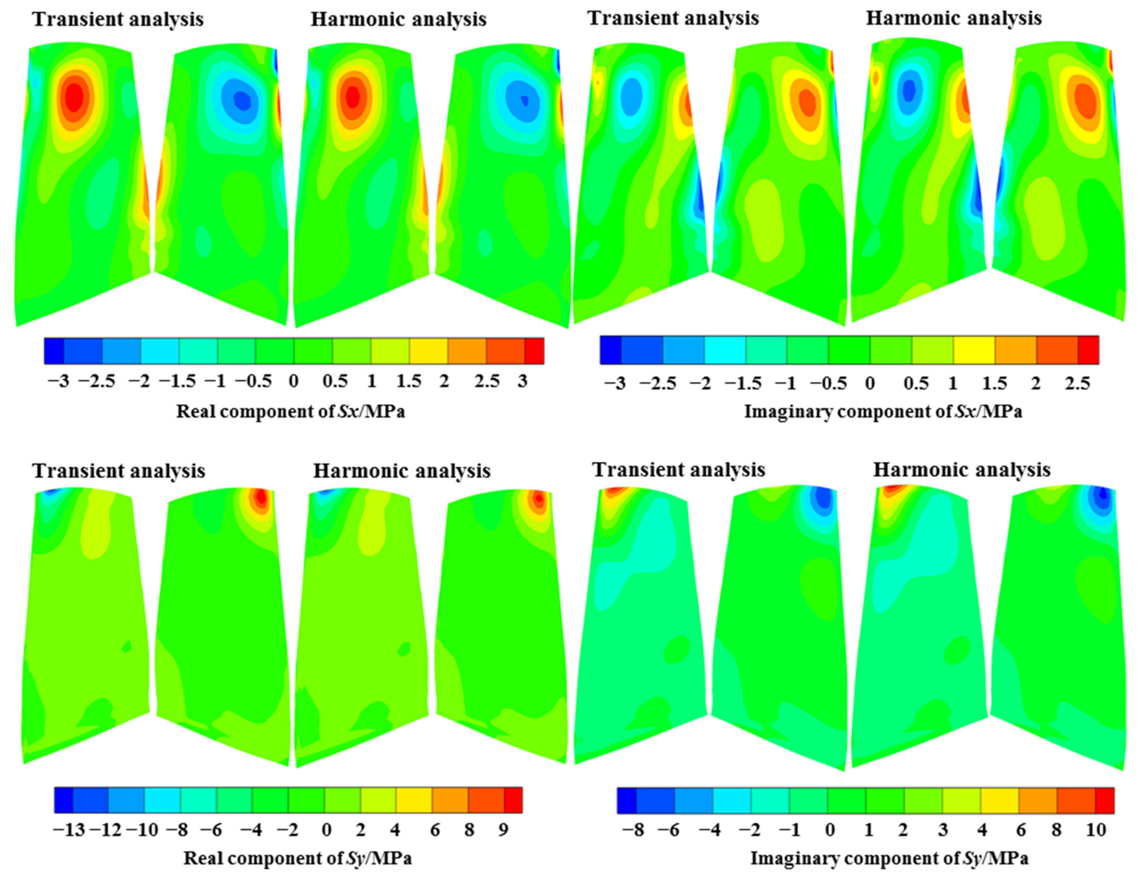
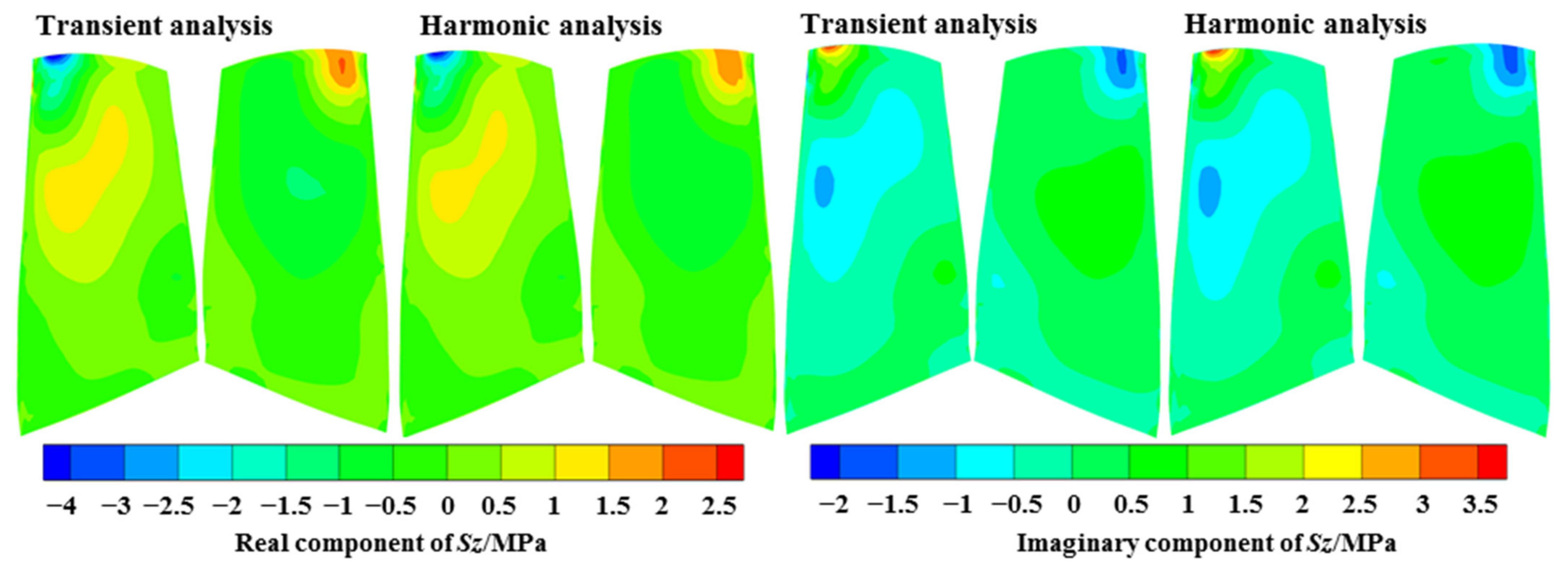
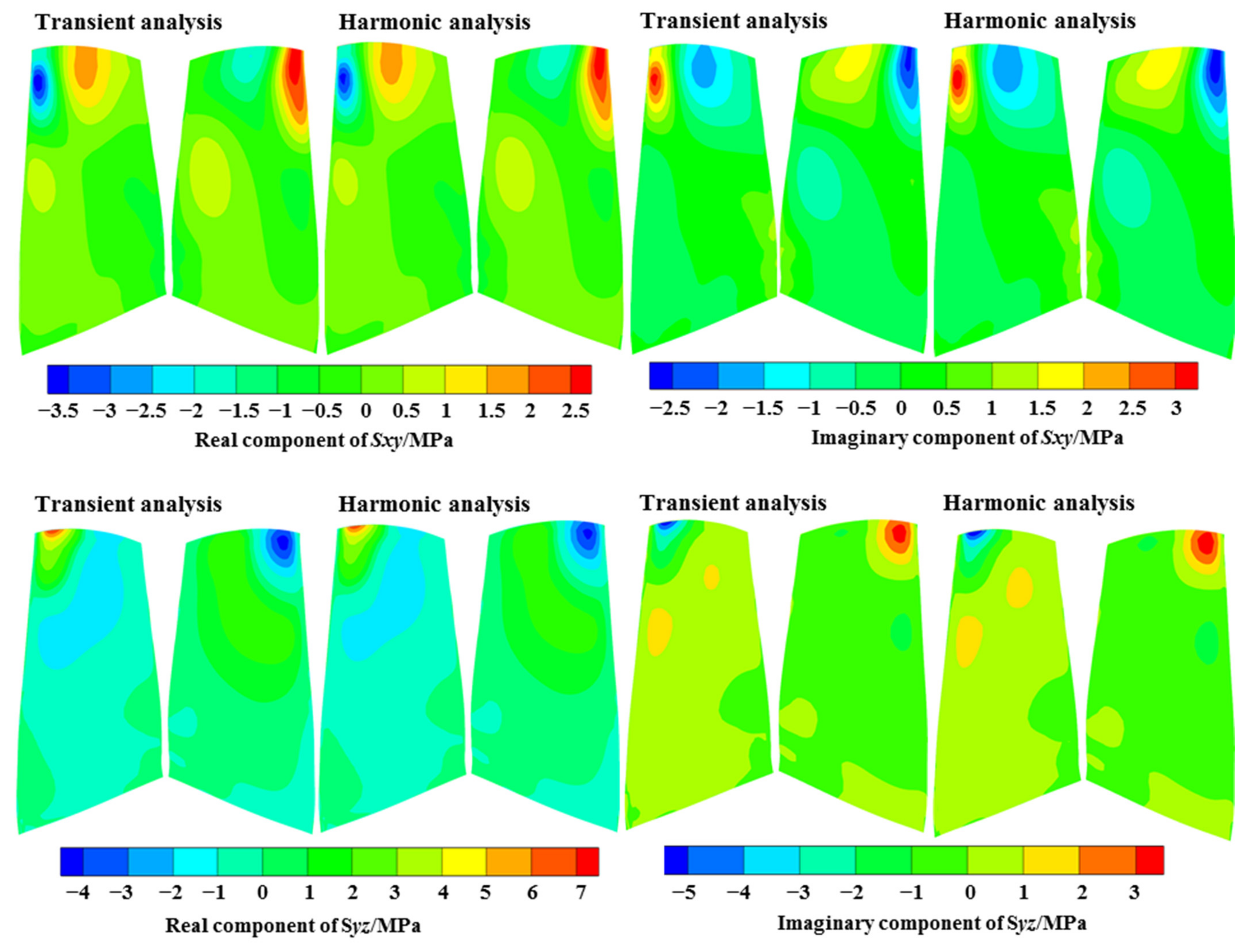
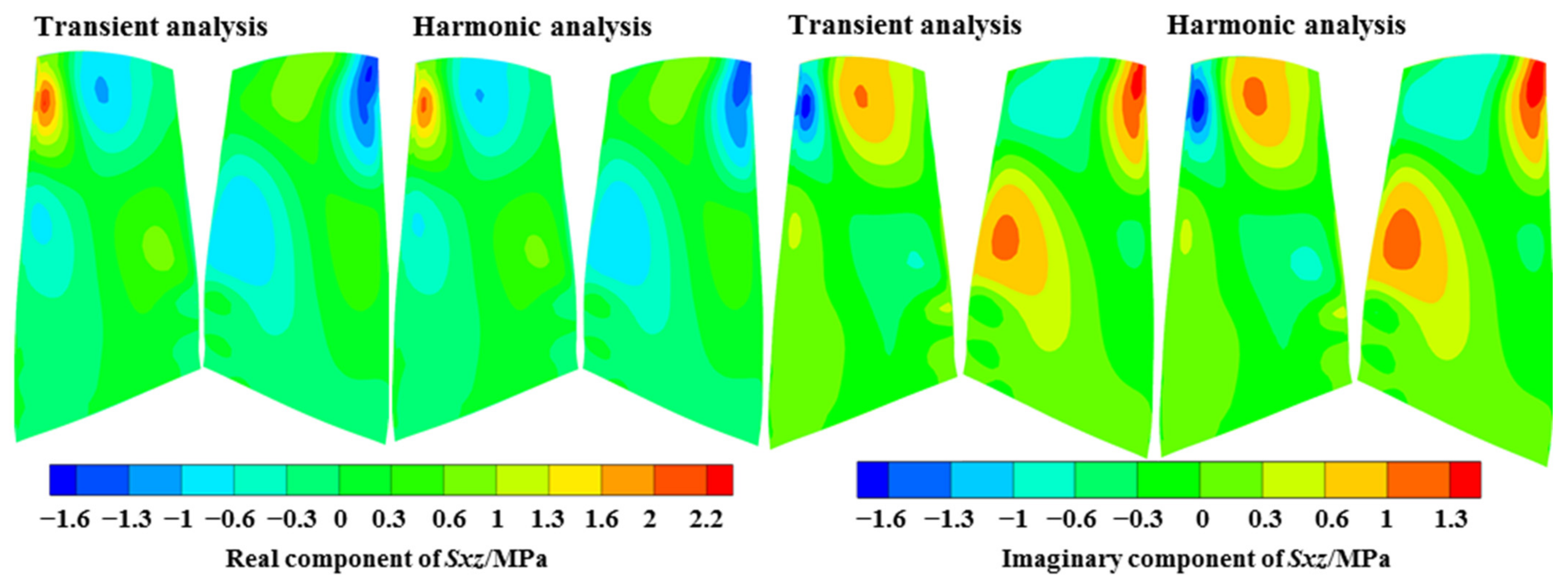
4.3. Harmonic Forced Response
5. Conclusions
Author Contributions
Funding
Institutional Review Board Statement
Informed Consent Statement
Data Availability Statement
Conflicts of Interest
References
- Kovachev, N.; Waldherr, C.U.; Mayer, J.F.; Vogt, D.M. Prediction of Aerodynamically Induced Blade Vibrations in a Radial Turbine Rotor Using the Nonlinear Harmonic Approach. ASME J. Eng. Gas Turb. Power 2018, 141, 021007. [Google Scholar] [CrossRef]
- Canepa, E.; Formosa, P.; Lengani, D.; Simoni, D.; Ubaldi, M.; Zunino, P. Influence of Aerodynamic Loading on Rotor-Stator Aerodynamic Interaction in a Two-Stage Low Pressure Research Turbine. J. Turbomach. 2007, 129, 765–772. [Google Scholar] [CrossRef]
- Efstathios, K.; Chunlei, L. Dynamic Response of a Turbulent Cylinder Wake to Forced Excitation. In Proceedings of the ASME 2009 Pressure Vessels and Piping Conference, Prague, Czech Republic, 26–30 July 2009; pp. 349–357. [Google Scholar]
- Nikola, K.; Tobias, R.M.; Christian, U.W.; Damian, M.V. Prediction of Low-Engine-Order Excitation Due to a Nonsymmetrical Nozzle Ring in a Radial Turbine by Means of the Nonlinear Harmonic Approach. J. Eng. Gas Turbines Power 2019, 141, 121004. [Google Scholar]
- Breard, C.; Green, J.; Imregun, M. Low-Engine-Order Excitation Mechanisms in Axial-Flow Turbomachinery. J. Propul. Power 2003, 19, 704–712. [Google Scholar] [CrossRef]
- Seinturier, E. Forced Response Computation for Bladed Disks Industrial Practices and Advanced Methods. In Proceedings of the 12th IFToMM World Congress, Besancon, France, 18–21 June 2007; pp. 1–17. [Google Scholar]
- He, L. Fourier Methods for Turbomachinery Applications. Prog. Aerosp. Sci. 2010, 46, 329–341. [Google Scholar] [CrossRef]
- Ning, W.; He, L. Computation of unsteady flows around oscillating blades using linear and non-linear harmonic Euler methods. J. Turbomach. 1998, 120, 508–514. [Google Scholar] [CrossRef]
- Hall, K.; Thomas, J.; Clark, W.S. Computation of Unsteady Nonlinear Flows in Cascades Using a Harmonic Balance Technique. AIAA J. 2002, 40, 879–886. [Google Scholar] [CrossRef] [Green Version]
- Erdos, J.; Alzner, E. Numerical Solution of Periodic Transonic Flow through a Fan Stage. AIAA J. 1977, 15, 1559–1568. [Google Scholar] [CrossRef]
- He, L. An Euler Solution for Unsteady Flows around Oscillating Blades. J. Turbomach. 1990, 112, 714–722. [Google Scholar] [CrossRef]
- Connell, S.; Hutchinson, B.; Galpin, P.; Campregher, R.; Godin, P. The Efficient Computation of Transient Flow in Turbine Blade Rows Using Transformation Methods. In Proceedings of the ASME Turbo Expo 2012: Turbine Technical Conference and Exposition, Copenhagen, Denmark, 11–15 June 2012; pp. 2631–2640. [Google Scholar]
- Sharma, G.; Zori, L.; Connell, S.; Godin, P. Efficient Computation of Large Pitch Ratio Transonic Flow in a Fan with Inlet Distortion. In Proceedings of the ASME Turbo Expo 2013: Turbine Technical Conference and Exposition, San Antonio, TX, USA, 3–7 June 2013; pp. 1–11. [Google Scholar]
- Rai, M.M. Navier-Stokes Simulations of Rotor-Stator Interactions Using Patched and Overlaid Grids. J. Propul. Power 1987, 3, 387–396. [Google Scholar] [CrossRef]
- Galpin, P.F.; Broberg, R.B.; Hutchinson, B.R. Three-Dimensional Navier Stokes Predictions of Steady State Rotor/Stator Interaction with Pitch Change. In Proceedings of the Third Annual Conference of the CFD Society of Canada, Banff, AB, Canada, 25–27 June 1995. [Google Scholar]
- Gerolymos, G.; Michon, G.; Neubauer, J. Analysis and Application of Chorochronic Periodicity in Turbomachinery Rotor/Stator Interaction Computations. J. Propul. Power 2002, 18, 1139–1152. [Google Scholar] [CrossRef]
- Giles, M. Calculation of Unsteady Wake/Rotor Interaction. J. Propul. Power 1988, 4, 356–362. [Google Scholar] [CrossRef]
- Zori1, L.; Galpin, P.; Campregher, R.; Morales, J.C. Time-Transformation Simulation of a 1.5 Stage Transonic Compressor. J. Turbomach. 2017, 139, 071001.1–071001.11. [Google Scholar] [CrossRef]
- Cornelius, C.; Biesinger, T.; Zori, L.; Campregher, R.; Galpin, P.; Braune, A. Efficient Time Resolved Multistage CFD Analysis Applied to Axial Compressors. In Proceedings of the ASME Turbo Expo 2014: Turbine Technical Conference and Exposition, Düsseldorf, Germany, 16–20 June 2014; pp. 1–14. [Google Scholar]
- Cornelius, C.; Biesinger, T.; Galpin, P.; Braune, A. Experimental and Computational Analysis of a Multistage Axial Compressor Including Stall Prediction by Steady and Transient CFD Methods. J. Turbomach. 2014, 136, 061013.1–061013.12. [Google Scholar] [CrossRef]
- Ansys CFX Version 19.2 Documentation; ANSYS Inc.: Canonsburg, PA, USA, 2021.
- Carta, F.O. Coupled Blade-Disk-Shroud Flutter Instabilities in Turbojet Engine Rotors. ASME J. Eng. Gas Turb. Power 1967, 89, 419–426. [Google Scholar] [CrossRef]
- Moffatt, S.; He, L. Blade Forced Response Prediction for Industrial Gas Turbines: Part 1—Methodologies. In Proceedings of the ASME Turbo Expo 2003, Collocated with the 2003 International Joint Power Generation Conference, Atlanta, GA, USA, 16–19 June 2003; pp. 407–414. [Google Scholar]
- Brian, J.O.; Steven, W.S.; Chengzhi, S.; Christophe, P.; Robert, G.P. Circulant Matrices and Their Application to Vibration Analysis. Appl. Mech. Rev. 2014, 66, 040803. [Google Scholar]


| Method | Passages Required | Total Time-Steps | Relative Mesh Nodes | Relative Cost in Memory | Relative Computing Time |
|---|---|---|---|---|---|
| TT | 4 | 6384 | 1 | 1 | 1 |
| TM | 83 | 6384 | 20.7 | 1106.6 | 19.8 |
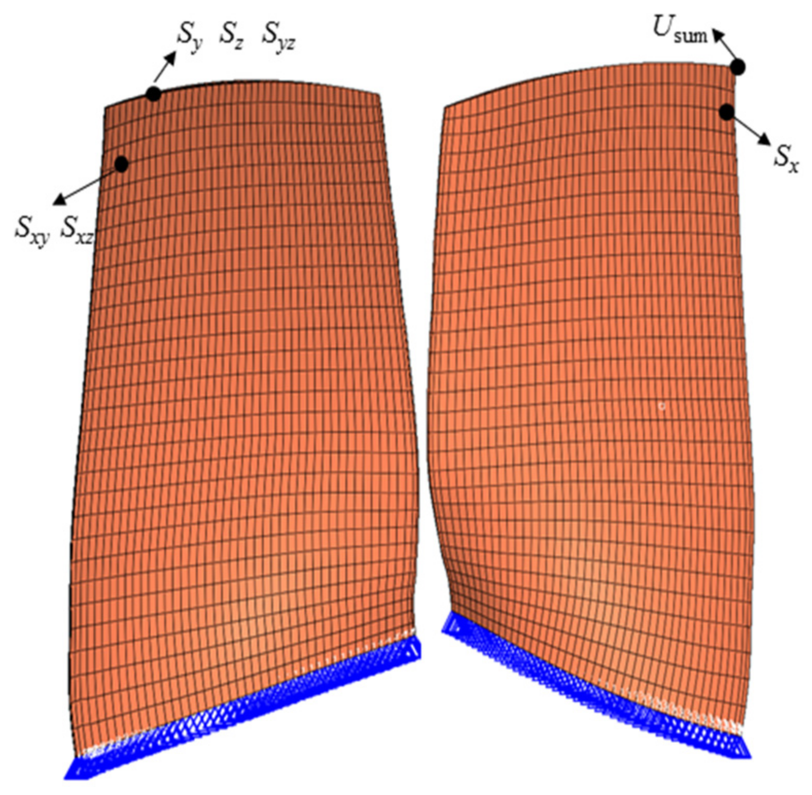
| Method | Normalized Resonance Frequency 1 | Usum /mm | Sx /MPa | Sy /MPa | Sz /MPa | Sxy /MPa | Syz /MPa | Sxz /MPa | Computing Time |
|---|---|---|---|---|---|---|---|---|---|
| Transient | 0.7419 | 0.102 | 4.37 | 17.30 | 5.49 | 5.12 | 9.14 | 2.84 | ~30 h |
| Harmonic | 0.7415 | 0.103 | 4.29 | 17.34 | 5.52 | 5.15 | 9.17 | 2.86 | <5 min |
| Error/% | −0.05 | 0.98 | −1.83 | 0.23 | 0.55 | 0.59 | 0.33 | 0.70 |
Publisher’s Note: MDPI stays neutral with regard to jurisdictional claims in published maps and institutional affiliations. |
© 2021 by the authors. Licensee MDPI, Basel, Switzerland. This article is an open access article distributed under the terms and conditions of the Creative Commons Attribution (CC BY) license (https://creativecommons.org/licenses/by/4.0/).
Share and Cite
Zhang, X.; Wang, Y.; Jiang, X. An Efficient Approach for Predicting Resonant Response with the Utilization of the Time Transformation Method and the Harmonic Forced Response Method. Aerospace 2021, 8, 312. https://doi.org/10.3390/aerospace8110312
Zhang X, Wang Y, Jiang X. An Efficient Approach for Predicting Resonant Response with the Utilization of the Time Transformation Method and the Harmonic Forced Response Method. Aerospace. 2021; 8(11):312. https://doi.org/10.3390/aerospace8110312
Chicago/Turabian StyleZhang, Xiaojie, Yanrong Wang, and Xianghua Jiang. 2021. "An Efficient Approach for Predicting Resonant Response with the Utilization of the Time Transformation Method and the Harmonic Forced Response Method" Aerospace 8, no. 11: 312. https://doi.org/10.3390/aerospace8110312