Article

On a Novel Approximate Solution to the Inhomogeneous Euler–Bernoulli Equation with an Application to Aeroelastics

by
Dominique Fleischmann
1,† and
László Könözsy
2,*,†
1
Centre for Aeronautics, Cranfield University, Cranfield, Bedfordshire MK43 0AL, UK
2
Centre of Computational Engineering Sciences, Cranfield University, Cranfield, Bedfordshire MK43 0AL, UK
*
Author to whom correspondence should be addressed.
These authors contributed equally to this work.
Aerospace 2021, 8(11), 356; https://doi.org/10.3390/aerospace8110356
Submission received: 25 September 2021 / Revised: 16 November 2021 / Accepted: 18 November 2021 / Published: 22 November 2021
(This article belongs to the Special Issue Advances in Aerospace Sciences and Technology II)

Abstract

:
This paper focuses on the development of an explicit finite difference numerical method for approximating the solution of the inhomogeneous fourth-order Euler–Bernoulli beam bending equation with velocity-dependent damping and second moment of area, mass and elastic modulus distribution varying with distance along the beam. We verify the method by comparing its predictions with an exact analytical solution of the homogeneous equation, we use the generalised Richardson extrapolation to show that the method is grid convergent and we extend the application of the Lax–Richtmyer stability criteria to higher-order schemes to ensure that it is numerically stable. Finally, we present three sets of computational experiments. The first set simulates the behaviour of the un-loaded beam and is validated against the analytic solution. The second set simulates the time-dependent dynamic behaviour of a damped beam of varying stiffness and mass distributions under arbitrary externally applied loading in an aeroelastic analysis setting by approximating the inhomogeneous equation using the finite difference method derived here. We compare the third set of simulations of the steady-state deflection with the results of static beam bending experiments conducted at Cranfield University. Overall, we developed an accurate, stable and convergent numerical framework for solving the inhomogeneous Euler–Bernoulli equation over a wide range of boundary conditions. Aircraft manufacturers are starting to consider configurations with increased wing aspect ratios and reduced structural weight which lead to more slender and flexible designs. Aeroelastic analysis now plays a central role in the design process. Efficient computational tools for the prediction of the deformation of wings under external loads are in demand and this has motivated the work carried out in this paper.

1. Introduction

Pressures to minimise the environmental impact of air travel have led to aircraft manufacturers becoming focused on reducing the fuel consumption of the next generation of civil transport aircraft. Manufacturers are starting to consider configurations with increased wing aspect ratios and reduced structural weight, and this is leading to more structurally flexible designs [1,2,3,4]. Engineers can no longer assume that the airframe is rigid, and it becomes increasingly important to take account of the aeroelastic behaviour earlier in the design process. Efficient computational tools for use at the conceptual design stage for the prediction of the deformation of wing beams with representative physical properties under varying external loads are now in demand. Such tools are also applicable to the aeroelastic analysis of helicopter rotor blades and wind turbines. Recent research works related to aeroelastic analysis were conducted by Amoozgar et al. [5], Vazhayil Thomas et al. [6], Rajpal et al. [7], Tsushima et al. [8], Rong et al. [9], Sommerwerk et al. [10] and Qin et al. [11]. It is with these developments in mind that the present work was undertaken.
This paper addresses the problem of finding approximate solutions to the inhomogeneous fourth-order Euler–Bernoulli partial differential Equation (PDE) using the finite difference method for application to the analysis of flexible aircraft at the conceptual design stage.
Work to exploit the Calculus and partial differential equations to analyse the strength and deformation of structures began in the 18th Century. A good survey of the history of this field of engineering was prepared by Timoshenko [12]. Leonhard Euler (1707–1783) and Daniel Bernoulli (1700–1782) worked in collaboration to apply the mathematical tools of the Calculus to the analysis of the strength and deformation of beams under an external load, and this work was continued and refined by Claude-Louis Navier (1785–1836). A major result of their work is the fourth-order Euler–Bernoulli PDE.
In recent decades, the Euler–Bernoulli equation has been used in engineering analysis to predict the dynamic oscillatory behaviour of structures under loads that vary in both space and time. In particular, the equation has been successfully applied to the prediction of the oscillatory deformation of aircraft wings, helicopter rotor blades, wind turbines and hydrofoils undergoing unsteady fluid-dynamic loading. Good introductions to this topic and its application in the field of aerospace design are given by Murua and Palacios [13], Hodges [14], Wright and Cooper [15] and Bisplinghoff et al. [16,17].
In recent years, a large amount of work has been conducted regarding the application of the Euler–Bernoulli equation to the emerging technological field of nano-structures—especially micro-electro mechanical systems (MEMSs). We refer the reader to the work of Fernandez et al. [18], and for the use of changes of coordinates to take account of very large deflections, we refer the reader to the work of Tari et al. [19]. Regarding new techniques in the numerical solution of the equation, Scuciato et al. [20,21] used a time domain boundary element method to solve the inhomogeneous equation for beams with mechanical properties that are independent of length along the beam.
Of particular interest is the work of Li and Sun [22] who derived a finite difference scheme for the Timoshenko-coupled PDEs. While the Timoshenko equations are applicable to a wider class of problems than those of the Euler–Bernoulli equation, the work presented in [22] contains several simplifying assumptions that means their results are only applicable to problems where the beam stiffness E, second moment of the area of cross-section I, Timoshenko coefficient κ , cross-sectional area A, and shear modulus G are independent of the distance along the beam span. These assumptions were not made in the present work.
Analytic solutions exist for the homogeneous version of the Euler–Bernoulli PDE and for certain specific boundary conditions. In contrast, solving the equation for arbitrary boundary and initial conditions using analytic techniques is very difficult, and it is more practical in these cases to use a numerical approach to find approximate solutions. Numerical techniques based on modal analysis were widely used and a large body of knowledge now exists for this approach. Our motivation for pursuing the work described in this paper was a desire to avoid the a priori choice of the mode basis functions. The result was an alternative solution technique based on the finite difference method that makes no assumptions regarding the modes of deformation, and does not use a component summation approach. By developing an approximation method based on an independent theory, the two methods can be compared and used to validate each other. In addition to the practical aspects of comparing predictions and computational techniques, having two alternative theoretical bases may lead to a greater depth of understanding of the underlying equation.
In this paper, we derived an analytical solution to the Euler–Bernoulli equation with boundary conditions relevant to application in aeroelastic analysis. Other authors have provided analytical solutions for different applications of Euler–Bernoulli and Timoshenko equations. Kundu and Ganguli [23] carried out an analysis on the weak solution of the Euler–Bernoulli equation taking into account an axial force. The inclusion of an axial force term in the Euler–Bernoulli equation has particular application to the analysis of helicopter rotor blades and wind turbine blades where the dynamics were strongly influenced by the centrifugal force (see the work of Fleischmann et al. [24]). Li et al. [25] provided a bending solution of Timoshenko beams based on the solutions of the homogeneous Euler–Bernoulli equation. Analytical formulations of the stochastic Euler–Bernoulli beam equation were derived by Yuan [26]. One can find more analytical solutions to different applications in the works of Miao et al. [27], Xu et al. [28], Sumelka et al. [29], Baghani et al. [30], Ma and Gao [31], Dongming and Liu [32], Ndogmo [33], Djondjorov [34], and Elishakoff and Livshits [35].
Reddy and El Borgi [36] proposed a formulation of the governing equations of Euler–Bernoulli and Timoshenko beams taking into account moderate rotations. They considered the length scales of the materials relying on the Eringen’s non-local theory using a nonlinear finite element approach. Further details on the development of the non-local theory of Euler–Bernoulli and Timoshenko beams were discussed by Sarkar and Reddy [37], Khodabakhshi and Reddy [38], Fernandez et al. [18] and Roque et al. [39]. The Euler–Bernoulli theory was also applied to the analytical and numerical investigation of the behaviour of micro- and nanobeams (see the works of Ghayesh et al. [40]; Demir and Civalek [41]; Rahaeifard [42]; Semnani et al. [43]; Shafiei et al. [44]; Nejad and Hadi [45]; Nejad et al. [46]; Mehdi and Nikkhah [47]; Abadi and Daneshmehr [48]; Mehdi and Nikkhah [47]; Mehdi [49]; Eltaher et al. [50]; Roque et al. [39]; and Kong et al. [51,52]. Other nanoscale applications have been found in the literature, and it is important to mention that Khajeansari et al. [53] derived an explicit solution for bending nanowires using the Euler–Bernoulli beam theory.
The consideration of time-varying load distribution is of central interest in engineering applications. The Euler–Bernoulli beams in conjunction with moving loads were studied by Giunta et al. [54] and Prasad [55]. A dynamic analysis was carried out by Shangand et al. [56] using a generalised finite element formulation and a time-dependent boundary element method was employed by Scuciato et al. [20,21]. There is ongoing research into the identification of the basis function coefficients of approximate solutions to the Euler–Bernoulli equation which was carried out by Lerma and Hinestroza [57], Kawano [58], Marinov and Vatsala [59,60].
In an attempt to improve fuel efficiency, aircraft manufacturers are considering wings with much higher aspect ratios. To achieve the planform area required, such large wing-spans are needed that folding wing tips are considered to allow access to airport gates. The aeroelastic behaviour and design of the folding geometry and stiffness is of important concern, and this has been investigated using a finite element approximation to the Euler–Bernoulli equation in [61,62]. In some concepts, spring stiffness is introduced at the hinge line for the purpose of gust alleviation, and research in this area is presented in [63,64].
We begin this paper with a short review of the Euler–Bernoulli equation and the development of a numerical approach for solving it. For comparison purposes, the full derivation of an analytical solution to the homogeneous version of the equation with a very specific set of boundary and initial conditions is presented in Appendix A. The results of computations using the new finite difference algorithm presented towards the end of this paper will then be compared against this analytical solution, and this forms part of the validation of the algorithm. We followed this by documenting a commonly used (but to the best of knowledge, unpublished) systematic method for deriving expressions for finite difference approximations of derivatives of any given degree to any given order of accuracy, and we provided a snippet of Matlab® computer code in a dataset linked to this paper that implements the method. A write-up of the method in the form of post-graduate teaching notes prepared by Miskandarani can be found, e.g., in [65]. We applied the method to the construction of an explicit finite difference solution scheme for the Euler–Bernoulli equation for the application to the analysis of beams in the presence of time-varying external loads with a velocity-dependent damping term and taking into account mass, the second moment of area, and elastic modulus beam structural properties, that arbitrarily vary with the distance along the beam.
The Lax–Richtmyer stability criteria were applied to the scheme to derive an upper limit on Δ t to ensure numerical stability. The concern is that such a restriction on the size of Δ t might render this finite difference scheme computationally inefficient. However, this concern has proved unfounded in practice. To strengthen confidence in the validity of the scheme and its implementation, we present the results of a grid sensitivity study using the Richardson generalised extrapolation method (as can be seen in the work of Roache in [66]) and these results demonstrated that the scheme is indeed grid convergent.
We followed this by presenting the results of three sets of computer experiments. The first set simulated the behaviour of the unloaded beam. Careful choice of the initial and boundary conditions allowed us to compare the results with the homogeneous analytical solution provided in the earlier part of this paper. The second set of computer experiments simulated the time-domain behaviour of a beam with properties chosen to represent the slender flexible wing structure of a generic aircraft. This consisted of the stiffness and mass distributions varying along the length of the beam, while subjected to inertial and fluid-dynamic loading during a gust encounter. It is crucial to appreciate that in this work the external load distribution due to the fluid-dynamic lift is dependent on the surface geometry, which in turn depends on the beam deformation. In this way, the deformation feeds back into the external load distribution. The third set of computer experiments was used to validate the finite difference method against experimental data. Experiments were conducted as part of background research at Cranfield University to measure the static deformation of the tip of a horizontally oriented aluminium alloy beam cantilevered at one end as different transverse point loads are applied to the opposite end. Computer simulations were conducted with the replicated boundary conditions and the results were compared with the experimental results.
This paper concludes by summarising the main findings and giving suggestions for further work to expand the applicability of the methods presented.

2. Governing Equations and Solution Methodology

In this section, we develop a numerical approach for solving the inhomogeneous Euler–Bernoulli equation. The derivation of an analytical solution to the homogeneous version of the Euler–Bernoulli equation with simple boundary and initial conditions is provided in Appendix A which we use in Section 3 to validate the numerical scheme developed in this work. For the inhomogeneous equation, when the function describing the transverse loading is taken into account, the unsteady numerical method was employed and a stability analysis was also carried out. We assumed that (a) deformations remain elastic which means that the deformations are small and that strain in the material remains within the elastic range; (b) plane sections remain plane, which means that cross-sections do not distort out of plane during bending; (c) the material properties are isotropic; and (d) the beam is not subject to any longitudinal loading. These assumptions restrict the validity of the Euler–Bernoulli theory to those cases where the deformation is small relative to the length of the beam. This means that nonlinearities associated with large deflections are neglected in the work presented here. In such cases, the beam bending theory of Timoshenko can be considered.
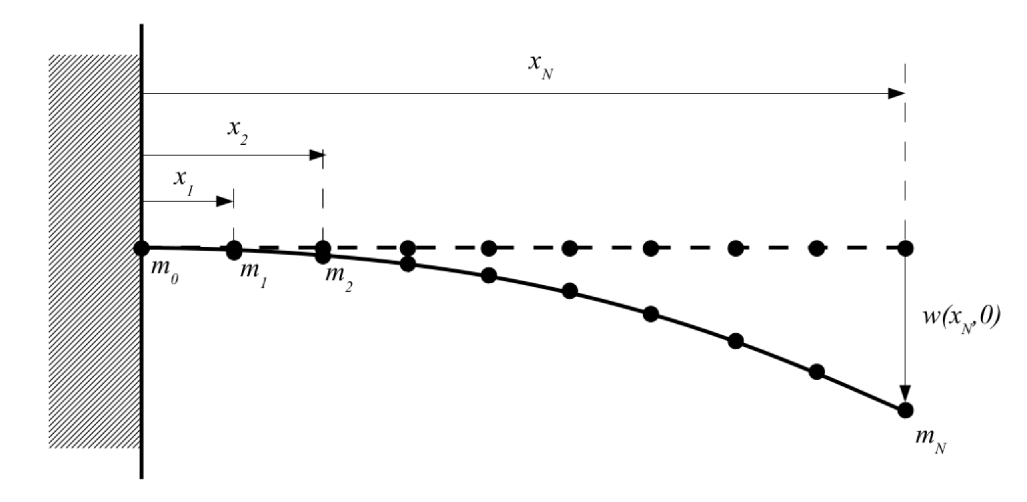
Under the assumptions stated above, the Euler–Bernoulli equation can be used to predict the dynamic deformation behaviour of a slender beam under a laterally applied distributed load. The inhomogeneous Euler–Bernoulli equation in a rectangular Cartesian coordinate system (see Figure 1) can be written as
t μ w t + 2 x 2 E I 2 w x 2 = q x , t ,
where E = E ( x ) is the modulus of elasticity of the beam material, I = I ( x ) is the second moment of area of cross-section of the beam taken about the neutral axis parallel to the plane z = 0 , μ = μ ( x ) is the mass-per-unit length along the beam, the function w = w ( x , t ) is the lateral deflection of the beam as a function of distance along the beam x and time t, and  q = q ( x , t ) is the given external force per metre applied to the beam as a function of distance along the beam x and time t.
In real-world engineering applications, mechanical damping causes the amplitude of oscillation of a beam under a steady externally applied load to decrease over time and the deformation tends towards an equilibrium deformation profile. To capture this behaviour, we included a velocity-dependent damping term in our simulation. We assumed that the mechanical damping force was linearly proportional to velocity, and directly the opposite to the local deflection velocity. Including the damping term and re-arranging, we have:
2 t 2 w x , t = q x , t μ x 1 μ x 2 x 2 E x I x 2 x 2 w x , t β t w x , t ,
where β is the non-dimensional damping coefficient.

2.1. Development of a Numerical Approach for Solving the Inhomogeneous Euler–Bernoulli Equation

In this section, we develop a numerical scheme for solving the inhomogeneous Euler–Bernoulli Equation (1) by using finite difference approximations. We emphasise that the proposed approach overcomes the assumption that the deformation function is the linear superposition of basis mode shapes, and thus we avoid the necessity of defining the shape of the mode basis functions at the outset. The numerical scheme is applied to a single beam experiencing a transverse load distribution q ( x , t ) in a single direction (see Figure 2). We note that the load distribution q ( x , t ) is not a follower distribution, and therefore the method described here is limited to conditions where values of w / x are small.
Geometric nonlinearities were taken into account in this work by permitting arbitrary distributions of structural properties as a function of distance along the beam x, and these distributions are sampled at discrete positions corresponding to the beam nodes of the finite difference method described below. These variable structural properties are E = E ( x ) ; I = I ( x ) ; μ = μ ( x ) ; and  q = q ( t , x ) . If the distribution of these beam properties rapidly changes, our approach would be to increase the fineness of the discretisation and increase the number of nodes in the finite difference scheme.
The purpose of the time-marching finite difference scheme is to determine w ( x i , t n + 1 ) , given w ( x i , t n ) , and w ( x i , t n 1 ) for all i { 0 , , N } , where we have adopted the subscript n in keeping with the convention used in finite difference schemes for indexing the time levels. We combined finite difference approximations for the various derivatives in Equation (1) to form the finite difference version of the Euler–Bernoulli equation and we re-arranged the equation to obtain an expression for w ( x i , t n + 1 ) in terms of w ( x i , t n ) and w ( x i , t n 1 ) for all i { 0 , , N } .
We emphasise that the function w ( x , t ) represents the deformation of the initially straight beam, and is measured perpendicularly to the straight beam. Since no account was taken of the change in the angle of the beam as w varies, this approach necessarily ignores the preservation of beam length. This is an additional reason for the imposition of the small w / x condition of the method.
We assume that the beam is initially at rest so that:
t w x i , 0 = 2 t 2 w x i , 0 = 0 , i { 0 , , N } .
Using numerical techniques to propagate the geometry of the beam from one discrete time level to the next involves solving the Euler–Bernoulli equation for the unknown node displacement at each node. It is important to note that great care must be taken in computing the numerical approximation of the derivatives in Equation (1). To perform computations for nodes near the ends of the beam, it is necessary to fill the stencil beyond the ends with artificially generated values of w. We call these artificial values "ghost" points and we call the artificially generated nodes at which these values are taken "ghost" nodes. We will show that contrarily to being an impediment to the method, the values of w at the ghost points are fully determined by the boundary conditions.
We proceed to substitute for partial derivatives in the inhomogeneous Equation (2) using finite difference expressions. Without loss of generality, we assumed Δ t is a constant for all time levels and Δ x is a constant for each point along the beam. Evaluating the inhomogeneous Euler–Bernoulli Equation (2) at the discrete coordinates x i and t n , we obtain:
2 t 2 w x i , t n = q x i , t n μ x i 1 μ x i 2 x 2 E x i I x i 2 x 2 w x i , t n β t w x i , t n .
Substituting central second-order accurate temporal and spatial discretisation schemes, we can write the finite difference approximation of Equation (4) as
w x i , t n + 1 2 w x i , t n + w x i , t n 1 Δ t 2 + O Δ t 2 = q x i , t n μ x i 1 μ x i S x i , t n β w x i , t n + 1 w x i , t n 1 2 Δ t + O Δ t 2
where x n + 1 = x n + Δ x , etc., and where S is defined as
S x i , t n = 1 Δ x 2 F x i 1 2 x 2 w x i 1 , t n b 2 F x i 2 x 2 w x i , t n c + F x i + 1 2 x 2 w x i + 1 , t n f + O Δ x
where the superscripts b, c, and f denote backward, central, and forward second derivatives to third-order accuracy, respectively, and where F ( x i ) = E ( x i ) I ( x i ) . For the three second-degree spatial derivatives in Equation (6), we employed third-order accurate finite difference discretisation schemes, and we write:
S x i , t n = 1 Δ x 4 1 12 F x i 1 w x i 4 , t n + 1 3 F x i 1 w x i 3 , t n + 1 2 F x i 1 + 1 6 F x i w x i 2 , t n + 5 3 F x i 1 8 3 F x i w x i 1 , t n + 11 12 F x i 1 + 5 F x i + 11 12 F x i + 1 w x i , t n + 8 3 F x i 5 3 F x i + 1 w x i + 1 , t n + 1 6 F x i + 1 2 F x i + 1 w x i + 2 , t n + 1 3 F x i + 1 w x i + 3 , t n 1 12 F x i + 1 w x i + 4 , t n + O Δ x ,
where the central third-order accurate spatial second-degree derivative in Equation (6) is estimated by
f 2 x 1 12 f x 2 Δ x + 4 3 f x Δ x Δ x 2 + 5 2 f x + 4 3 f x + Δ x 1 12 f x + 2 Δ x Δ x 2 + O Δ x 3 ,
the backward third-order accurate scheme is estimated by
f 2 x 1 12 f x 3 Δ x + 1 3 f x 2 Δ x Δ x 2 + 1 2 f x Δ x 5 3 f x + 11 12 f x + Δ x Δ x 2 + O Δ x 3 ,
and the forward third-order accurate discretisation is estimated by
f 2 x 11 12 f x Δ x 5 3 f x + 1 2 f x + Δ x Δ x 2 + 1 3 f x + 2 Δ x 1 12 f x + 3 Δ x Δ x 2 + O Δ x 3 .
The process of forming the finite difference representation of a partial differential equation requires that each derivative in the original equation be replaced by a finite difference approximation of a given order of accuracy. The order of accuracy directly affects the number of terms in the Taylor expansion that are taken into account. It can be a laborious task to derive these approximations by hand. We used an algorithm suitable for computer automation in the derivations of the expressions in Equations (8)–(10). Such algorithms are frequently taught in university courses but we did not find them in the published literature. For this reason, we included a derivation of the algorithm in Appendix B. A Matlab® script that implements this algorithm can be found in the MDPI code database (see Appendix E).
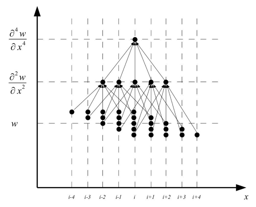
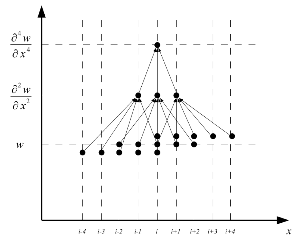
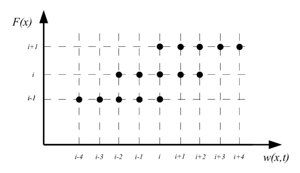
A specific combination of left, centre, and right finite differences are contained in Equation (6). This choice of biases is largely based on our computational experience. We tried to use other combinations of biases, but these attempts exhibited unexpected oscillatory characteristics that do not correspond to physically realistic behaviour found in the experiment. For example, replacing the biases in Equation (6) with centred finite differences throughout results in the wild unbounded continual oscillatory behaviour of the function w that appears right from the start of the simulation. The authors believe that the suitability of the choice of biases in the different terms is associated with the route of information propagation through the algorithm. To illustrate our heuristic justification, we present plots of stencils of the nodes used in two different simulations (see Figure 3 and Figure 4). A derivative sampling scheme that gives rise to wild oscillatory behaviour is presented in Figure 3 and the derivative sampling finally chosen for this work is shown in Figure 4.
It is important to note that the oscillatory scheme (see Figure 3) required the use of third-order accuracy for the approximation of both second-degree derivatives, while the physically realistic scheme (see Figure 4) only requires third-order accuracy for the approximation of the first second-degree derivative. This suggests that taking higher-order accuracy alone does not lead in itself to the better capture of physical phenomena.
Re-arranging Equation (5) and dropping the order terms gives:
w x i , t n + 1 1 1 + β Δ t 2 Δ t 2 μ x i q x i , t n Δ t 2 μ x i S x i , t n + β Δ t 2 1 w x i , t n 1 + 2 w x i , t n ,
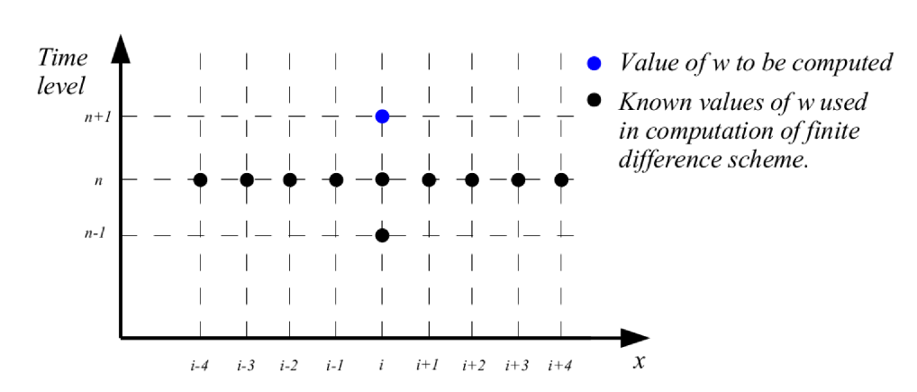
where S x i , t n is given by Equation (7). The stencil of Equation (11) is illustrated in Figure 5.
The outputs of the algorithm are approximations of the deflection function w at discretely sampled intervals along the length of the beam x and at discretely sampled times t greater than 0. In the next subsection, we derive sufficient criteria for the finite difference scheme to be stable.

2.2. Extension of the Lax–Richtmyer Stability Criteria to the Fourth-Order Euler–Bernoulli Equation

There are several established methods for determining conditions on the spatial step size Δ x and the time-step size Δ t in PDEs such that instabilities are avoided. An existing method suitable for use in explicit parabolic finite difference schemes of second-order linear PDEs is given in [67].
In order to assure the stability of the fourth-order Euler–Bernoulli equation presented in this paper, we propose to extend the application of the Lax–Richtmyer stability criteria to higher-order schemes to obtain an upper limit on Δ t which is dependent on Δ x . We focus on the coefficient of the w ( x i , t n ) term in Equation (11). According to the Lax–Richtmyer criteria, the finite difference scheme will likely be stable if the coefficient has a positive pre-sign.
First, considering the multiplicative term in Equation (11), we see that:
1 1 + β Δ t 2 > 0
for all β > 0 and all Δ t > 0 , so it remains to consider the coefficients inside the square braces in Equation (11). Grouping all terms in w ( x i , t n ) and explicitly writing this condition, we require that:
2 1 μ x i Δ t 2 Δ x 4 11 12 F x i 1 + 5 F x i + 11 12 F x i + 1 > 0 ,
which leads to the inequality for a stable time-step size of the discretised Euler–Bernoulli equation given by
Δ t < Δ x 2 2 μ x i 11 12 F x i 1 + 5 F x i + 11 12 F x i + 1 .
Since this condition must hold for the whole beam, we see that Δ t must satisfy:
Δ t < min i { 0 , N } Δ x 2 2 μ x i 11 12 F x i 1 + 5 F x i + 11 12 F x i + 1 .
The Lax–Richtmyer stability criteria states that the pre-signs of all coefficients of w depending on Δ x and Δ t on the right-hand side of Equation (11) should be positive. Taking the coefficient of w ( x i 4 , t n ) as an example, we have:
a w x i 4 , t n = 1 1 + β Δ t 2 1 μ x i Δ t 2 Δ x 4 1 12 F x i 1 ,
which is always positive for all Δ x and Δ t by virtue of the fact that F ( x j ) is positive for all j { 1 , , N } . Similar expressions exist for the coefficients of w ( x i + 4 , t n ) , w ( x i 1 , t n ) , and w ( x i + 1 , t n ) .
For the coefficients of w ( x i 3 , t n ) , w ( x i 2 , t n ) , w ( x i + 2 , t n ) , and w ( x i + 3 , t n ) , the coefficients are negative irrespective of the choice of Δ x and Δ t , and so the Lax–Richtmyer stability criteria can never be satisfied by these terms. It may appear that this jeopardises the stability of the algorithm. However, some terms with a negative pre-sign are in fact necessary; otherwise, the function w ( x i , t n ) would be a monotonic increasing function of x i and t n .

2.3. Specification of Boundary Conditions and Values of Functions F and W at the Ghost Nodes

As illustrated in Figure 6, to compute w ( x i , t n + 1 ) for i { 1 , , N } in Equation (11), two ghost values of F are required beyond each end of the beam. We defined these values by linear extrapolation as
F ( x 1 ) = F ( x 0 ) + [ F ( x 0 ) F ( x 1 ) ] , F ( x 2 ) = F ( x 1 ) + [ F ( x 1 ) F ( x 0 ) ] ,
and:
F ( x N + 1 ) = F ( x N ) + [ F ( x N ) F ( x N 1 ) ] , F ( x N + 2 ) = F ( x N + 1 ) + [ F ( x N ) F ( x N 1 ) ] .
For the cantilevered beam considered in this paper, the physical boundary conditions on w are:
w x 0 , t n = 0 , x w x 0 , t n = 0 , 2 x 2 w x N , t n = 0 and 3 x 3 w x N , t n = 0 n N .
To ensure that the gradient of the w function vanishes at x 0 , we set w ( x 1 , t n ) = w ( x 0 , t n ) = w ( x 1 , t n ) = 0 for all n N . We also set w ( x 2 , t n ) = 0 for all n N so the first and second left hand ghost points are determined by the second boundary condition. Considering the third boundary condition, we have:
w ( x N + 1 , t n ) 2 w ( x N , t n ) + w ( x N 1 , t n ) ( Δ x ) 2 = 0 n N ,
and re-arranging this gives:
w ( x N + 1 , t n ) = 2 w ( x N , t n ) w ( x N 1 , t n ) ,
so the first right ghost point is determined by the third boundary condition. Finally, we consider the fourth boundary condition, and we require:
w ( x N + 2 , t n ) 2 w ( x N + 1 , t n ) + 2 w ( x N 1 , t n ) w ( x N 2 , t n ) ( Δ x ) 3 = 0 ,
and re-arranging this gives:
w ( x N + 2 , t n ) = 2 w ( x N + 1 , t n ) 2 w ( x N 1 , t n ) + w ( x N 2 , t n ) ,
so the second right ghost point is determined by the fourth boundary condition. The third and fourth left and right ghost points remain to be determined. We arbitrarily constrain the third and fourth left-hand ghost point values of w to be zero. We set the third and fourth right-hand ghost points using linear extrapolation as
w ( x N + 3 , t n ) = 2 w ( x N + 2 , t n ) w ( x N + 1 , t n ) ,
and:
w ( x N + 4 , t n ) = 2 w ( x N + 3 , t n ) w ( x N + 2 , t n ) .
The finite difference scheme described in this paper together with the boundary conditions were implemented in a Matlab® script which is included in the dataset linked to this paper (see Appendix E). All simulations were performed using this script.

3. Results and Discussions

3.1. Grid Sensitivity Study for the Fourth-Order Euler–Bernoulli Equation

We begin by showing that the finite difference scheme for approximating the fourth-order Euler–Bernoulli equation with damping is grid convergent. We present the results of a grid sensitivity study using the Richardson generalised extrapolation method as detailed in [66]. For this activity, we used a uniformly applied constant external load function q ( x , t ) = q , a constant beam structural properties E ( x ) = E and I ( x ) = I , and a damping coefficient β = 10 throughout. We examined the accuracy of the finite element scheme as Δ x is varied. For each choice of Δ x , the value of Δ t is chosen such that the Lax–Richtmyer criteria were met for the w ( x i , t n ) term for all i { 0 , , N } . We performed four simulations of the finite difference scheme and we identified variables associated with each of the different simulations by the subscript j.
We selected four values of Δ x denoted by Δ x j for j { 1 , 2 , 3 , 4 } such that:
Δ x 1 L 0.08 , Δ x 2 L 0.04 , Δ x 3 L 0.02 and Δ x 4 L 0.01 ,
so that, in general, Δ x j + 1 Δ x j / 2 for each j { 1 , 2 , 3 } . The number of nodes for each j is given by
N j L Δ x j ,
and in order to keep the mass of the beam M constant and independent of j, the node mass M j ( x i ) = M j is taken to be:
M j = M N j .
Now, we select a fixed time t > t 0 where t 0 is the time at the start of a simulation, and a fixed C ( 0 , 1 ) . Then, we define a node index i j such that i j / N j C for each j { 1 , 2 , 3 , 4 } . In this way, the  i j t h node is at approximately the same point along the beam for all values of j. We proceeded to perform the four simulations of the finite difference scheme, one for each Δ x j , and consider the predicted value of the function w at the point ( x i j , t ) for each simulation j. For a more convenient notation, we set:
w j w ( x i j , t )
for each simulation.
Since the Lax–Richtmyer stability inequality in (15) contains a ( Δ x ) 2 multiplicative term, it is clear that, as the value of Δ x reduces, a smaller step size in t must be chosen to ensure numerical stability. Thus, for each Δ x j , there is a corresponding stable time step and we denote this by Δ t j . This in turn implies that the number of iterations required to estimate w j will strongly depend on j.
Once the simulations are completed and the values of w j are known, we form the three norms given by
n 1 , 2 = w 1 w 2 w 2 , n 2 , 3 = w 2 w 3 w 3 and n 3 , 4 = w 3 w 4 w 4 .
The corresponding grid convergence indices (GCIs) G j are then given by
G j = n j , j + 1 Δ x j Δ x j + 1 p 1 , j { 1 , 2 , 3 } ,
where p is the order of accuracy of the finite difference scheme. In our case, since the scheme is first-order accurate in space, we set p = 1 . According to the theory presented in [66], if  G j < G j + 1 for j = 1 and j = 2 , then the finite difference scheme is grid convergent.
The finite difference simulation was performed using the Matlab® script with the parameters presented in Table 1.
The results of the simulations are presented in Table 2 below.
The norms are then given by
n 1 , 2 = w 1 w 2 w 2 = 1.0043 1.1881 1.1881 = 0.1547 n 2 , 3 = w 2 w 3 w 3 = 1.1881 1.2609 1.2609 = 0.0577 n 3 , 4 = w 3 w 4 w 4 = 1.2609 1.2957 1.2957 = 0.0268 .
Finally, computing the G C I values, we have:
G 1 = n 1 , 2 Δ x 1 Δ x 2 1 1 = 0.1547 1 = 0.1547 , G 2 = n 2 , 3 Δ x 2 Δ x 3 1 1 = 0.0577 1 = 0.0577 G 3 = n 3 , 4 Δ x 3 Δ x 4 1 1 = 0.0268 1 = 0.0268 .
These are good results. We see that G 1 > G 2 > G 3 , which implies that the finite difference scheme fulfils the criteria for grid convergence given by Richardson [66]. We are concerned that while the values of w j demonstrate grid convergence, this analysis does not measure the number of oscillations of the beam tip before t . To verify whether the number of oscillations is stable between cases, a second grid convergence study was performed with β set to zero throughout, and the results are presented in Table 3. Table 3 includes the extra column indicating the number of oscillations performed by the vibrating beam during the simulation time. The spread of values of w j was explained by the fact that the measurement was taken at different phases of oscillation. The amplitudes of oscillation were very closely matched.
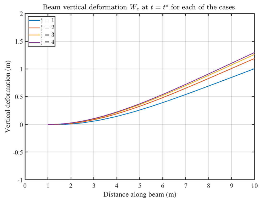
Figure 7 presents the beam deformation distributions for each of the four grid convergence study cases at time t = t .
This grid convergence study was performed with the algorithms implemented in Matlab®. On a PC with 8 Intel Core i7-7800X @3.50GHz processors, one iteration of the fourth case of the grid convergence study (101 nodes) takes approximately five microseconds to execute, as measured by the Matlab® tic and toc functions. This way, to compute one second of beam dynamics for this case takes approximately 10 s of computation time.
In the next sub-section, we describe activities undertaken to compare the predictions using the finite difference approach with the analytical solution.

3.2. Comparison of the Simulation Results with an Analytical Solution

Here, we compare the finite difference algorithm with the analytical solution of the homogeneous equation derived in Appendix A. We compare the time histories of the tip deflection of a beam without damping predicted by both approaches for the specific boundary and initial conditions of a cantilevered beam with initial deflection equal to the first mode shape and without an external load. The geometry and structural properties used here are the same as for the beam in the grid convergence study presented above.
For the purposes of validating the finite difference algorithm against the homogeneous Euler–Bernoulli equation, we start with Equation (A28) and set the initial geometry of the beam to:
w ( x , 0 ) = w 1 ( x , 0 ) = cos α 1 x cosh α 1 x + sin α 1 L sinh α 1 L cos α 1 L + cosh α 1 L sin α 1 x sinh α 1 x ,
with H 1 = 1 . As such, we dramatically simplify the form of the function w ( x , 0 ) without compromising the method of validation of the finite difference method. Then, we define the exact analytic function w a as
w a ( x , t ) = ( cos α 1 x cosh α 1 x . + sin α 1 L sinh α 1 L cos α 1 L + cosh α 1 L sin α 1 x sinh α 1 x ) cos t E I μ α 1 4 .
For a beam of length L = 10 m we, find that the first positive value of α (denoted α 1 ) satisfies Equation (A16) to be 0.1875.
With E = 70.0 × 10 9 (aluminium), I = 6.67 × 10 5 and M = 80 (beam mass evenly distributed over all the nodes), it follows that:
w a ( x , t ) = ( cos α 1 x cosh α 1 x . + sin α 1 L sinh α 1 L cos α 1 L + cosh α 1 L sin α 1 x sinh α 1 x ) cos t E I μ α 1 4 = ( cos 0.1875 x cosh 0.1875 x . + sin 1.8751 sinh 1.8751 cos 1.8751 + cosh 1.8751 sin 0.1875 x sinh 0.1875 x ) cos 26.857 t .
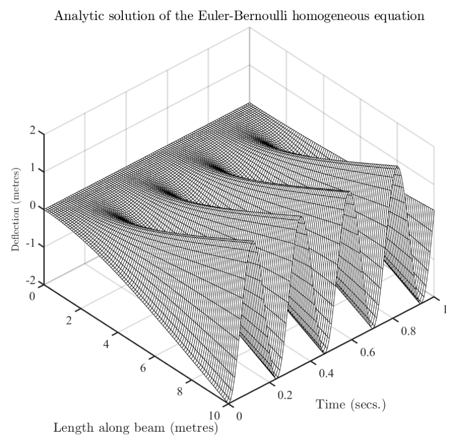
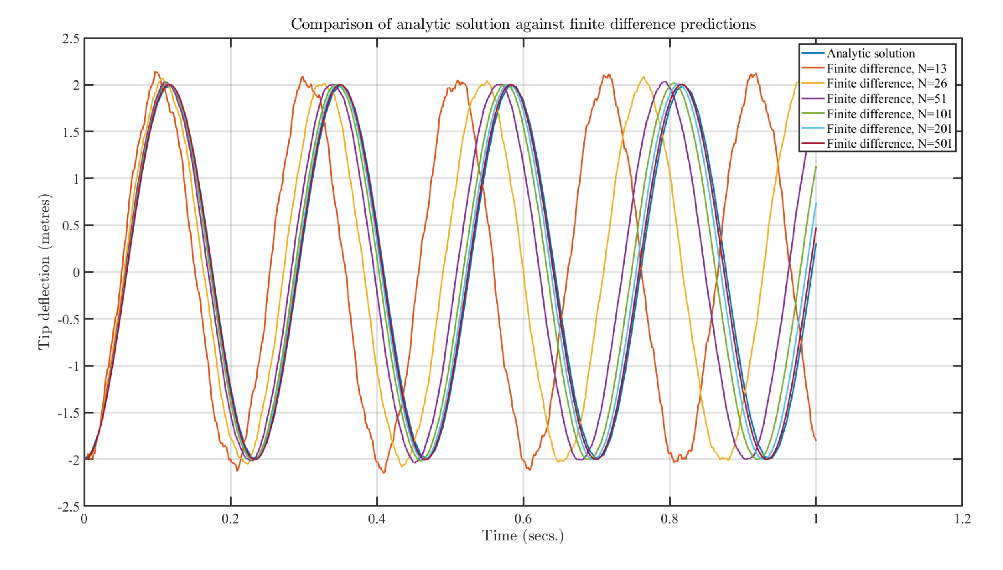
Figure 8 presents the deflection of the 10-m cantilevered beam in free vibration using Equation (36) as a function of length along the beam x and time t. Figure 9 presents a comparison of the tip excursions predicted for this cantilevered beam in free vibration using Equation (36) and using the finite difference algorithm presented above. It is clear that the natural frequency of vibration predicted using the finite difference approach is higher than the analytical solution when fewer nodes are used, and as the number of nodes increases, the predicted frequency decreases towards the analytical solution.

3.3. Application of the Finite Difference Scheme to a Realistic Case of a Commercial Aircraft Wing in a Gust Encounter

As part of the certification procedure for any new design of commercial aircraft, the design authority (manufacturer) is obliged to demonstrate that the aircraft can satisfactorily operate when subjected to gusts and turbulence during flight. A set of standard vertical gust velocity profiles is specified by the certification authority for use in the certification process, and one of these profiles is often referred to as the “ one minus cosine” profile. A full description of the gust specification can be found in the Federal Airworthiness Administration publication [68]. The one minus cosine profile is a vector field defined as
v ( x , y , z ) = 0 i + 0 j + M 2 1 cos ( 2 π x x 0 / S ) k , if x 0 x x 0 + S 0 i + 0 j + 0 k , otherwise ,
where i , j , and k are the unit vectors in the three orthogonal axes x, y, and z, respectively, and where M and S are fixed scalar constants.
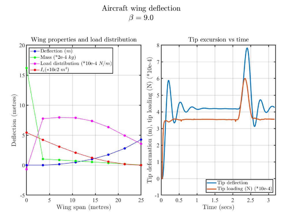
Here, we present the results of a set of simulations of the finite difference algorithm applied to the case of a wing of a large commercial passenger aircraft encountering a one minus cosine gust during steady forward flight to predict the vertical deformation of one of the wings. We assumed the aircraft is symmetric with regard to the vertical centre-line plane, and that the wings are built into a rigid fuselage; therefore, it is only necessary to analyse one wing (the right wing in this case). We estimated distributions of mass, the second moment of area, and Young’s modulus from the general engineering experience, and we used an inhomogeneous source function predicted by unsteady potential flow theory for the gust encounter. Figure 10 shows the results of the simulation that starts at time t = 0 with zero initial deflection; that is, w ( x , 0 ) = 0 for all x.
The Euler–Bernoulli Equation (1) models the transverse translation deformation of the beam. It does not explicitly incorporate any coupling with twisting deformation. In physical aero-elastic scenarios, there is strong interaction between the bending and twisting. For the case described in this section, only bending was considered. This was done to specifically study the finite difference method in isolation. This way, we were sure that the dynamical deformation of the beam observed here was only due to the algorithm presented in this paper.
An Unsteady Vortex Lattice Method (UVLM) developed by one of the authors and implemented in the software package Flexit and described in [24] was used to predict the inhomogeneous source function q ( x , t ) . The UVLM was described in [69]. The gust velocity profile (which varies with the position in the flow field) affects the boundary conditions on the UVLM as the aircraft flies through the gust. These changes in the boundary conditions affected the resulting predicted pressure distribution over the wing. This change in pressure distribution in turn changes the Euler–Bernoulli source function q ( x , t ) , and the finite difference method predicts a change in the deflection function w ( x , t ) of the wing spar. It is crucial to appreciate that this change in w ( x , t ) results in a change in the wing aerodynamic geometry and a new bound vortex geometry. On the next time step, the UVLM uses this new bound vortex geometry and the resulting pressure distribution prediction is based on this new geometry.
The unsteady nature of the computation ensures that there is a feedback between the fluid-dynamic forces and the wing geometry. The resulting simulation is therefore not simply a forced vibration, but rather a full time-varying fluid–structure interaction (FSI) simulation. In the present work, we used the Flexit software code to perform these calculations. More details of the FSI algorithms used in this software are described in reference [24].
For the purpose of this demonstration of the algorithm, we discretised the wing structural beam into just eight nodes. For a typical aeroelastic analysis, many more nodes would be used. The left-hand plot shows a snapshot of the deformation geometry at the end of the simulation. The right-hand plot shows the wing tip deflection and the value of the load applied along the wing as they vary throughout the simulation. The beam oscillates at the start of the simulation as the transverse load is initially applied. The amplitude of oscillation decreases, and at approximately 1 s, the oscillation has almost completely died out (and the tip deflection settles at approximately 4 m). At 2.2 s, the aircraft flies into the one minus cosine gust profile, and the potential flow theory predicts a transient increase in the transverse load. The finite difference algorithm then predicts a sudden increase in wing tip deflection peaking at approximately 8 m before again reducing to 4 m after the aircraft has flown past the gust profile.
The algorithm presented in this paper was included in a computational scheme where the twist and bending algorithms were executed in parallel. Implicit coupling takes place in this scheme because at each time step, the twist of the wing changes the UVLM panel geometry. This changes the predicted aero-dynamic pressure distribution, which in turn modifies the transverse load distribution q ( x , t ) in Equation (5). This coupling is not the immediate topic of this paper; however, the reader can see an illustration of the effect of the twisting on bending implemented in this way, in Appendix F.

3.4. Validation of the Finite Difference Approximation for the Euler–Bernoulli Equation against Experimental Data

3.4.1. Damping Coefficient β

For the established approach to predict the deformation of a beam using modal analysis, Rayleigh damping is usually used, with a mass damping coefficient μ and a stiffness damping coefficient λ . Estimates of μ and λ were established over many years by comparison between experiment and simulation.
For the approach developed in this work, the damping term is velocity-dependent, and we did not find a quantitative correspondence between the two damping methods.
As a result, it is difficult to estimate the correct value of the damping coefficient β that should be used when performing simulations with the finite difference algorithm. Structural damping is highly sensitive to the fine details of how the beam is constructed and assembled, and it is also sensitive to temperature. However, comparing the magnitudes of the damping force with typical external applied loads, it is clear that the effects of the damping forces are relatively small. In simulations for the design of an aircraft wing, the authors noted node deformation velocities of the order of 5 m per second. For a typical value of β of 10, this results in a damping force of 50 Newtons per node, while the external load applied to the node is approximately 1000 Newtons. Thus, the damping force accounts for approximately 5 percent of the response of the beam. If the error in the estimate of β is 50 percent, for instance, then the error in the simulation that results will only be 2.5 percent.

3.4.2. Comparison of Static Deflection Experiment with Finite Difference Simulation

As part of a general research project being performed by the Dynamics, Control and Simulation group at Cranfield University, experiments were conducted to determine the steady-state equilibrium tip deflection of a scale model of an aircraft wing spar clamped at the wing root when different transverse loads are applied at the tip. Here, we present the results of the work we performed to compare the static deflections measured during the experiments with simulations performed using the finite difference algorithms presented in this paper. Note that here we only compare the steady-state tip deflections once any transient oscillations have died out. More examples of the comparisons of beam bending theory with experimental data can be found in [70].
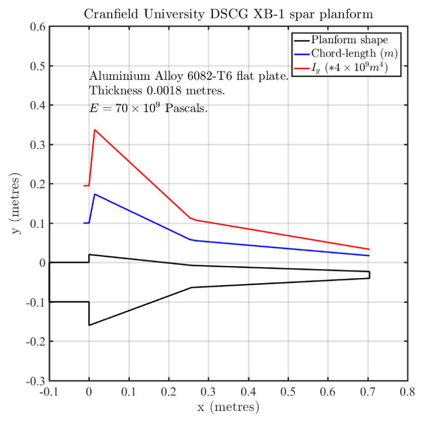
Figure 11 presents the geometry and structural properties of the wing spar model. The scale model under investigation is very simple, and consists of a single flat 6082-T6 specification aluminium plate, nominally measuring 2 mm in thickness with a rectangular cross-section. Accurate measurements of the sample conducted by the authors using a micrometre showed that the actual plate thickness varied from 1.7 mm to 1.9 mm along the length of the spar. Figure 12 shows the experimental set-up. Measurements of the tip deflection were recorded with a resolution of 1 mm. It is estimated that the measurement error is +/− 1 mm (2 σ ).
The wing spar model beam properties are also presented in Table 4.
In the experimental set-up, the wing was clamped ad built-in over the whole rectangular area on the left of the sample, and the larger irregular area was freely cantilevered. The geometry of the experiment, the relatively small tip loadings, and the small magnitudes of the deflections imply that the Euler–Bernoulli PDE can give a good approximation of the experiment.
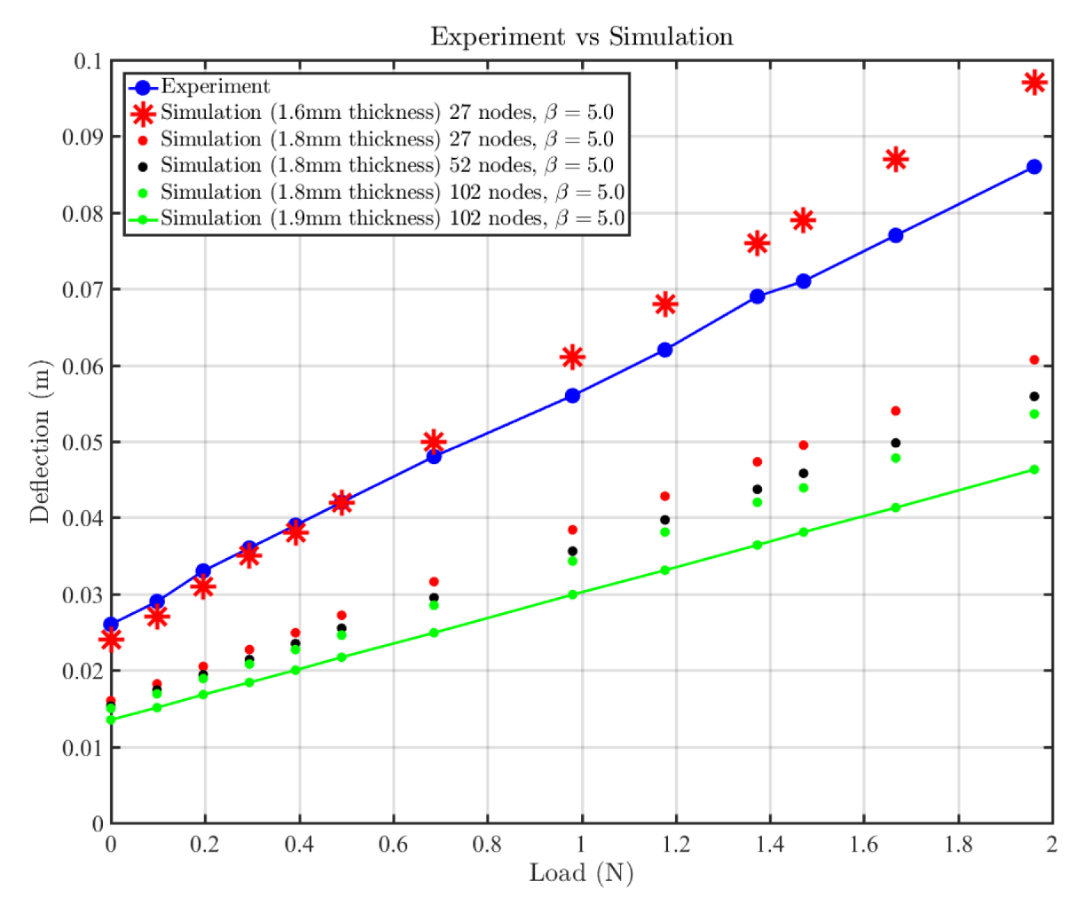
The dynamic simulation was performed using a number of nodes ranging from 27 to 102, a damping coefficient β of 5.0, and varying time steps (always satisfying the Lax–Richtmyer criteria), and we used the planform shape and second moment of area ( I y ) distributions of the actual test piece. Plate thicknesses ranging from 1.6 mm to 1.9 mm were investigated. The simulation began with zero initial deflection and the prediction was sampled after several million iterations after the oscillations completely damped out. Table 5 presents the loading cases and the corresponding deflections measured in the experiment and predicted by computer simulations using the finite difference algorithm.
The errors between the experimental results and the simulations are quite large. Figure 13 demonstrates that, as well as the magnitudes of deflection being in disagreement, there is also disagreement in the rate of the change of deflection with the load between the experiment and the simulations. Before passing judgement on the accuracy of the simulation, it is important to consider factors in the set-up of the experiment that may lead to these large discrepancies. These factors may include the impact of the inaccurate manufacture of the scale model such as variations in plate thickness, the arrangement for the clamping of the built-in spar, the method and accuracy of measurement of the deflection, and the existence of the pre-bend in the spar before the tests took place. In addition, the load was applied close to the tip, and not exactly at the tip of the beam. Figure 13 presents simulation data for a wide range of beam thicknesses in order to demonstrate that the algorithm is stable and robust over a wide range of input parameters.
We note that a small variation in the thickness of the aluminium sheet results in a large change in the predicted magnitudes of deflection. This is because the thickness is increased to the fourth power when computing the second moment of area. A change in thickness of 5 percent leads to a change in predicted deflection of 16 percent. Then, we note the error between the tip deflections predicted for zero tip loads and those measured in the test. These may be partially explained if the sample had a pre-bend before the test.
Of more concern, however, is the difference in the slopes of the load versus deflection curves. The slope of the simulation predictions is lower than that for the experiment, implying that the simulation overestimates the bending strength of the beam. Finally, we note that, as the number of nodes used in the simulation increases from 27 to 102 (for a plate thickness of 1.8 mm), the error in the predicted displacement in fact increases.

4. Conclusions and Future Work

Here, we discuss the main conclusions concerning the finite difference method presented in this paper. The finite difference method provides an alternative approach to the established mode shape analysis for the approximation of both the homogeneous and inhomogeneous versions of the Euler–Bernoulli equation. We demonstrated that the method can be applied to the analysis of aeroelastic phenomena in aircraft. The method results in excellent agreement with the analytical solution to the homogeneous Euler–Bernoulli equation. As the number of nodes increases, the finite difference algorithm appears to rapidly converge to the analytical solution. By applying the method to an idealised commercial aircraft wing subjected to external loading, we showed that the method can be applied in the general case where E, I, μ , and Δ x arbitrarily vary with x, and where the external load q arbitrarily varies with x and t. Indeed, the finite difference algorithm is stable and well behaved when performed for this realistic physical case. The equilibrium deformation predicted by the finite difference algorithm appears to give poor agreement with a particular set of experimental results. To form an accurate picture, comparison with other experimental results is recommended. We extended the application of the Lax–Richtmyer stability criteria to the fourth-order Euler–Bernoulli partial differential equation using a finite difference approximation. The stability of the finite difference algorithm is highly sensitive to the choice of forward, backward, and central finite difference approximations to the various derivatives. This paper considered the case of a simple beam geometry with one end cantilevered. By choosing different boundary conditions, it is possible to consider beams with different anchorings. The boundary conditions at the ends of the beam can easily be controlled by setting the values of w at the ghost nodes.
In this work, we considered the deflection function w : R 2 R that describes the scalar deflection in the z direction as a function of distance along the beam x and time t. We can extend the range of cases that can be analysed to beams subject to external load distributions and undergoing deflections in any direction in the y z plane (see Figure 1). These situations can be analysed by resolving the loads in the orthogonal y and z directions, and performing independent finite difference simulations in each of the resolved directions. The scheme described in this paper assumes that all the beam nodes are colinear. Real beams to be analysed in engineering applications are often not straight, and approximating them by a straight line is not appropriate. By expressing the Euler–Bernoulli equation in the generalised curvilinear coordinates, we can admit the analysis of beams with non-colinear nodes. The dynamical structural behaviour of a given beam undergoing angular rotation is different to that of the non-rotating beam. The effect of the angular velocity of a real beam is to increase its effective stiffness and increase the natural frequencies of vibration. By ignoring the effect of angular velocity, the predicted deformations will be too large and the oscillatory frequencies will be too low. To use the finite difference method for the analysis of rotating beams such as helicopter rotor blades, an extra term must be included in the PDE to account for centrifugal forces. See Appendix C for a description of the extra term required to take account of centrifugal forces. The effects of rotation of the cross-sections in the x z plane can become significant when larger deformations are experienced or when the shear modulus of the beam material is low. Developing a finite difference approach for the Timoshenko coupled equation will significantly extend the body of knowledge in two ways; firstly, it will provide an example of application of this method to coupled PDEs with two unknown functions of x and t (w and φ ); and secondly, it will provide a second method of predicting beam deflections and a comparison of the two methods will contribute to their validation. A description of the Timoshenko-coupled PDEs can be found in Appendix D. Finally, the choice of biases for the finite difference approximations should be further investigated.

Author Contributions

Conceptualisation, D.F.; methodology, L.K.; software, D.F.; validation, D.F. and L.K.; formal analysis, L.K.; investigation, D.F.; resources, not applicable; data curation, D.F.; writing—original draft preparation, D.F. and L.K.; writing—review and editing, L.K. and D.F.; visualisation, D.F.; supervision, L.K.; project administration, L.K.; funding acquisition, L.K. and D.F. All authors have read and agreed to the published version of the manuscript.

Funding

This research was funded by the Centre for Computational Engineering Sciences at Cranfield University under project code EEB6001R and by the Aerospace Technology Initiative, Innovate UK, and Airbus under the Grant Number 113041 of the Agile Wing Integration Project.

Institutional Review Board Statement

Not applicable.

Informed Consent Statement

Not applicable.

Data Availability Statement

Not applicable.

Acknowledgments

The authors are grateful to Douglas Muirden, Geert Kapsenberg, and Michael Strauss for their informal discussions that stimulated the ideas presented here. We would also like to acknowledge the IT support at Cranfield University, UK. We would also like to acknowledge the constructive comments of the anonymous reviewers of the MDPI Aerospace journal.

Conflicts of Interest

The authors declare no conflict of interest.

Abbreviations

The following abbreviations are used in this manuscript:
GCIGrid Convergence Index
MEMSMicro-Electronic Mechanical System
PDEPartial Differential Equation
Latin Nomenclature
ABeam Cross-Section Area ( m 2 )
AConstant in Analytical Solution (-)
BConstant in Analytical Solution (-)
CConstant in Analytical Solution (-)
CFraction of Beam Span Used in Richardson Analysis (−)
DConstant in Analytical Solution (-)
E ( x ) Young’s Modulus ( P a )
F ( x ) The Product of E and I ( k g m 3 / s )
F n Sequence of Constants in Analytical Solution (-)
G n Sequence of Constants in Analytical Solution (-)
G j Richardson Grid Convergent Index (−)
GBeam Shear Modulus ( P a )
H n Sequence of Constants in Analytical Solution (-)
I ( x ) Second Moment of Area ( m 4 )
iBeam Node Index (-)
i j Beam Node Index Used for j t h GCI (-)
LTotal Beam Length (m)
MThe Total Mass of the Beam ( k g )
MGust Constant ( m / s )
M j Beam Node Mass of j t h Richardson Simulation ( k g )
m i Mass of i t h Node ( k g )
NThe Number of Finite Difference Nodes along the Beam (-)
N j Number of Beam Nodes Of j t h Richardson Simulation (-)
nTime Step Index (-)
n i , j Auxiliary Quantity (−)
q ( x , t ) Beam External Loading Function ( k g / m s 2 )
SGust Constant (-)
SAuxiliary Quantity in Finite Difference ( k g / s 2 )
TAnalytic Deflection Function Dependent Only on Time (m)
tTime (s)
t Time at which Richardson Criteria Are Applied (s)
Δ t Finite Difference Time Step Size (s)
v Gust Velocity Vector Field ( m / s )
w ( x , t ) Beam Deflection Distance Function (m)
w a ( x , t ) Analytic Deflection Function (m)
XAnalytic Deflection Function Dependent Only on Distance Along Beam (m)
xDistance along the beam (m)
x i Distance Along Beam of i t h Node (m)
Δ x Distance Between Adjacent Nodes (m)
zDistance Perpendicular to Beam (m)
Greek Symbols
α n Auxiliary Constants in the Analytical Solution (-)
β Velocity-Dependent Damping Coefficient (-)
κ ( x ) Timoshenko Shear Modulus Coefficient (-)
λ Rayleigh Stiffness Damping Coefficient (-)
μ ( x ) Beam Mass per Unit Length ( k g / m )
μ Rayleigh Mass Damping Coefficient (-)
λ Auxiliary Constant in the Analytical Solution (-)
φ Angular Rotation of Beam Cross-Section ( r a d )

Appendix A. An Analytical Solution of the Homogeneous Euler–Bernoulli Equation for Validation Purposes

As part of the validation of our numerical work, we will compare our approximate numerical results against an exact analytical solution, and we derive the exact solution in this section.
For the general case, we might consider a rigidly cantilevered beam at one end (and otherwise free to deform) and then a time and span-wise varying transverse loading distribution function q ( x , t ) is applied. However, it is difficult to derive any analytical results when q ( x , t ) 0 and β 0 in Equation (2). Therefore, purely for validation purposes, we will consider here the special case of the homogeneous Equation ( q ( x , t ) = 0 ) and β = 0 with the rigidly cantilevered beam at one end. In this case, an analytical solution can be derived as outlined below.
While the homogeneous case is relatively simple, it does exercise much of the behaviour of the numerical method, and so provides a valuable means of improving confidence in the validity of the current work.
With these considerations in mind, we derived an analytical solution with boundary conditions where the beam is cantilevered at one end and the beam is free to oscillate without damping. The inhomogeneous case, in which the transverse load distribution is significant and varying in time and space will be subsequently discussed along with a comparison with experimental data.
Let us consider the homogeneous version of the Euler–Bernoulli equation with the beam property functions E, I, and μ independent of x and with the external force applied to the beam q x , t and the damping coefficient β both set to zero. In this case, we can write:
4 w x 4 = μ E I 2 w t 2 ,
which is often referred to as the free vibration equation. By applying the technique of separation of variables, an analytical solution to the homogeneous Equation (A1) can be found for a beam of length L of the form:
w x , t = X x T t ,
where the corresponding boundary conditions are:
X 0 = 0 , X 1 0 = 0 , and X 2 L = 0 , X 3 L = 0 ,
where we adopt the notation f p to denote the p t h derivative of the function f with respect to its independent parameter.
Substituting Equation (A2) into Equation (A1), we obtain:
T X ( 4 ) = μ E I X T ( 2 ) ,
and re-arranging Equation (A4) gives:
X ( 4 ) X = μ E I T ( 2 ) T ,
where the left side of Equation (A5) is only dependent on x and the right side is only dependent on t. Since x and t are independent variables, both sides must be equal to the same constant, e.g., λ . Thus, we have:
X ( 4 ) λ X = 0
and:
μ E I T ( 2 ) + λ T = 0 .
In this way, we expressed the partial differential Equation (A1) as two ordinary differential equations and a constant λ .
Beginning with the first ordinary differential Equation (A6) in x, we impose the constraint that we will only consider real-valued functions X. We justify this simplification by appealing to the fact that the deflection itself is real. We can also exclude the trivial and physically un-meaningful solutions when λ = 0 and λ < 0 , respectively. This leaves us with the case λ > 0 , and we consider the trial solution:
X x = A cos α x + B sin α x + C cosh α x + D sinh α x ,
where λ = α 4 . After differentiating the trial solution (A8) four times, we obtain:
X 1 x = α A sin α x + α B cos α x + α C sinh α x + α D cosh α x ,
X 2 x = α 2 A cos α x α 2 B sin α x + α 2 C cosh α x + α 2 D sinh α x ,
X 3 x = α 3 A sin α x α 3 B cos α x + α 3 C sinh α x + α 3 D cosh α x ,
and:
X 4 x = α 4 A cos α x + α 4 B sin α x + α 4 C cosh α x + α 4 D sinh α x .
We can see that X 4 x = α 4 X x = λ X x , so the trial solution given in Equation (A8) is indeed a solution to the ordinary differential Equation (A6). It remains to determine the coefficients A, B, C, and D, and the new constant α . To do this, we use the boundary conditions (A3) of the partial differential Equation (A1). By applying boundary conditions (A3) to our trial solution (A8) and imposing the condition that α 0 , we obtain:
A = C , B = D ,
thus:
A = B sin α L + sinh α L cos α L + cosh α L ,
and:
A = B cos α L + cosh α L sin α L sinh α L .
By combining Equations (A14) and (A15), we obtain the condition on α given by
1 + cos α L cosh α L = 0 .
There are countably infinite real (and therefore ordered) solutions to Equation (A16) for α and we denote them by α n , n N . The first few solutions can then be numerically approximated. For each n, the function:
X n x = A n cos α n x + B n sin α n x + C n cosh α n x + D n sinh α n x ,
is a solution to the ordinary differential Equation (A6). Substituting for B n , C n , and D n using Equations (A13) and (A15), we obtain:
X n x = A n cos α n x cosh α n x + A n sin α n x sinh α n x cos α n x + cosh α n x sin α n x sinh α n x ,
and these functions X n are often referred to as mode shapes. Since the linear sum of solutions to an ordinary differential equation is also a solution, it follows that, in general, any linear superposition of the mode shape functions is also a solution. Figure A1 presents the first five modes for A n = 1 , together with the total deformation shape given by n = 1 5 X n x . Note that, here, A n is simply a scaling constant.
Figure A1. First five mode shapes for a freely vibrating cantilevered beam.
Aerospace 08 00356 g0a1
We then turn our attention to the function T that must satisfy Equation (A7). Since λ = α 4 , it follows that there is a value of λ corresponding to each n, and we denote this value by λ n , and we write:
λ n = α n 4 , n N .
Thus, Equation (A7) becomes:
μ E I T n 2 + α n 4 T n = 0 ,
thus:
T n 2 = E I μ α n 4 T n , n N .
Assuming that the solution must be real-valued, for each n, we consider the trial solution:
T n t = F n cos t E I μ α n 4 + G n sin t E I μ α n 4 ,
where F n and G n are real-valued constants. By taking derivatives, we have:
T n 1 t = F n E I μ α n 4 sin t E I μ α n 4 + G n E I μ α n 4 cos t E I μ α n 4 ,
and:
T n 2 t = F n E I μ α n 4 cos t E I μ α n 4 G n E I μ α n 4 sin t E I μ α n 4 = E I μ α n 4 T n t ,
as required. Now, we recall that ( w / t ) ( x , 0 ) = 0 for all x ( 0 , L ) , so X n ( x ) T n ( 1 ) ( 0 ) = 0 , and this forces T n ( 1 ) ( 0 ) = 0 . Hence, G n = 0 , and so for each n N , we have:
T n t = F n cos t E I μ α n 4 .
Bringing together the expressions for X n and T n , the function w n x , t = X n x T n t can be written explicitly as
w n x , t = H n cos α n x cosh α n x cos t E I μ α n 4 + H n Z sin α n x sinh α n x cos t E I μ α n 4 ,
where:
Z = sin α n L sinh α n L cos α n L + cosh α n L
and where H n = A n F n . For each n N , the function w n ( x , t ) satisfies the homogeneous Euler–Bernoulli partial differential equation at (A1) and the boundary conditions w ( 0 , t ) = 0 and ( w / x ) ( 0 , t ) = 0 t > 0 , and the initial condition ( w / t ) ( x , 0 ) = 0 x [ 0 , L ] . For any given n, the function w n ( x , 0 ) may or may not be equal to the initial geometry of the beam f ( x ) . In fact:
w n x , 0 = H n cos α n x cosh α n x + H n Z sin α n x sinh α n x ,
for all x ( 0 , L ) only if f ( x ) is a constant multiple of:
cos α n x cosh α n x + Z sin α n x sinh α n x .
To satisfy a given initial condition f ( x ) such that w ( x , 0 ) = f ( x ) , in general, it may be possible to expand f ( x ) as a linear sum of the mode shapes on the interval ( 0 , L ) . We can express w ( x , 0 ) as
w x , 0 = f x = n = 0 H n cos α n x cosh α n x + Z sin α n x sinh α n x ,
where the constants H n are chosen accordingly.
Thus, the final form of the analytical solution to the homogeneous Euler–Bernoulli Equation (A1) can be written as
w x , t = n N H n cos α n x cosh α n x + Z sin α n x sinh α n x cos t E I μ α n 4 ,
where H n and α n for each n N are real constants. In Section 3.2, the values of w x , t given by Equation (A31) will be compared with approximations to w predicted by the numerical method to demonstrate the accuracy.

Appendix B. Algorithm for Deriving the Coefficients of a Finite Difference of a Given Degree and Order of Accuracy

The method described here is taught on undergraduate courses but we did not find it in the published literature. We followed the approach described by Iskandarani in [65].
We start by considering the Taylor series of a general smooth function f : [ a , b ] R for the value of f at x + m Δ x expanded about the point x ( a , b ) :
f ( x + m Δ x ) = f ( x ) + m Δ x 1 ! f ( 1 ) ( x ) + ( m Δ x ) 2 2 ! f ( 2 ) ( x ) + ( m Δ x ) 3 3 ! f ( 3 ) ( x ) + ,
where m is some integer in the set S = { l , , r } for l < r Z (so that the cardinality of S is r l + 1 ), and where f ( p ) denotes the p t h derivative of f with respect to x.
Now, we construct an equation of the form (A32) for each m S :
f ( x + l Δ x ) = f ( x ) + l Δ x 1 ! f ( 1 ) ( x ) + ( l Δ x ) 2 2 ! f ( 2 ) ( x ) + , f ( x + ( l + 1 ) Δ x ) = f ( x ) + ( l + 1 ) Δ x 1 ! f ( 1 ) ( x ) + ( ( l + 1 ) Δ x ) 2 2 ! f ( 2 ) ( x ) + , f ( x + r Δ x ) = f ( x ) + r Δ x 1 ! f ( 1 ) ( x ) + ( r Δ x ) 2 2 ! f ( 2 ) ( x ) + .
Then, we multiply each equation by a corresponding constant a m , m { l , , r } , where these constants are yet to be determined and we subtract a m f ( x ) from both sides of each equation to give:
a l f ( x + l Δ x ) a l f ( x ) = a l l Δ x 1 ! f ( 1 ) ( x ) + a l ( l Δ x ) 2 2 ! f ( 2 ) ( x ) + a l ( l Δ x ) 3 3 ! f ( 3 ) ( x ) + O ( Δ x ) 4 , a l + 1 f ( x + ( l + 1 ) Δ x ) a l + 1 f ( x ) = a l + 1 ( l + 1 ) Δ x 1 ! f ( 1 ) ( x ) + a l + 1 ( ( l + 1 ) Δ x ) 2 2 ! f ( 2 ) ( x ) + a l + 1 ( ( l + 1 ) Δ x ) 3 3 ! f ( 3 ) ( x ) + O ( Δ x ) 4 , a r f ( x + r Δ x ) a r f ( x ) = a r r Δ x 1 ! f ( 1 ) ( x ) + a r ( r Δ x ) 2 2 ! f ( 2 ) ( x ) + a r ( r Δ x ) 3 3 ! f ( 3 ) ( x ) + O ( Δ x ) 4 ,
where we introduced the O ( z ) notation to indicate a quantity of order z R .
When 0 S , the equation corresponding to m = 0 becomes:
a 0 f ( x + 0 ) a 0 f ( x ) = 0 ,
which is a trivial statement and provides no additional information. Thus, whenever 0 S , we omit the case m = 0 from the system of equations in (A34).
Constructing a single equation by summing all the equations in Equation (A34) (while omitting the equation corresponding to m = 0 ), we obtain:
m = l , m 0 r a m f ( x + m Δ x ) m = l , m 0 r a m f ( x ) = m = l , m 0 r m a m Δ x 1 ! f ( 1 ) ( x ) + m = l , m 0 r m 2 a m ( Δ x ) 2 2 ! f ( 2 ) ( x ) + m = l , m 0 r m 3 a m ( Δ x ) 3 3 ! f ( 3 ) ( x ) + O ( Δ x ) 4 .
Defining:
b k = m = l , m 0 r m k a m
we can write Equation (A36) as
m = l , m 0 r a m f ( x + m Δ x ) m = l , m 0 r a m f ( x ) = b 1 Δ x 1 ! f ( 1 ) ( x ) + b 2 ( Δ x ) 2 2 ! f ( 2 ) ( x ) + b 3 ( Δ x ) 3 3 ! f ( 3 ) ( x ) + O ( Δ x ) 4 .
Equation (A38) can be used to find an expression for the finite difference of f of any given degree and any order of accuracy in Δ x , and we proceed to demonstrate this below.
Given a degree p and an order of accuracy q, we can write an expression for f ( p ) ( x ) to q t h -order accuracy by requiring b s = 0 for s { 1 , , p 1 , p + 1 , , p + q 1 } and b p = 1 . With each of the coefficients b k constrained in this way, Equation (A38) becomes:
m = l , m 0 r a m f ( x + m Δ x ) m = l , m 0 r a m f ( x ) = ( Δ x ) p p ! f ( p ) ( x ) + O ( Δ x ) p + q .
Re-arranging the terms in Equation (A39), we have:
( Δ x ) p p ! f ( p ) ( x ) = m = l , m 0 r a m f ( x + m Δ x ) m = l , m 0 r a m f ( x ) + O ( Δ x ) p + q ,
thus:
f ( p ) ( x ) = p ! ( Δ x ) p m = l , m 0 r a m f ( x + m Δ x ) m = l , m 0 r a m f ( x ) + O ( Δ x ) p + q = p ! ( Δ x ) p m = l , m 0 r a m f ( x + m Δ x ) m = l , m 0 r a m f ( x ) + p ! O ( Δ x ) p + q ( Δ x ) p = p ! ( Δ x ) p m = l , m 0 r a m f ( x + m Δ x ) m = l , m 0 r a m f ( x ) + O ( Δ x ) q ,
where we use the fact that O ( a b + c ) / a c = O ( a b ) and O ( a ) = O ( a ) .
Thus, the expression:
p ! ( Δ x ) p m = l , m 0 r a m f ( x + m Δ x ) m = l , m 0 r a m f ( x )
is a finite difference approximation for f ( p ) ( x ) , accurate to q t h -order in Δ x .
The coefficients a m remain to be found, and we subsequently address this challenge.
We note that the conditions on the coefficients a m are
b 1 = m = l , m 0 r m a m = 0 , b 2 = m = l , m 0 r m 2 a m = 0 , b p 1 = m = l , m 0 r m p 1 a m = 0 , b p = m = l , m 0 r m p a m = 1 , b p + 1 = m = l , m 0 r m p + 1 a m = 0 , b p + q 1 = m = l , m 0 r m p + q 1 a m = 0 .
The equations at (A43) can be written in matrix form as -4.6cm0cm
l l 1 l 2 r 1 r l 2 ( l 1 ) 2 ( l 2 ) 2 ( r 1 ) 2 r 2 l p + q 1 ( l 1 ) p + q 1 ( l 2 ) p + q 1 ( r 1 ) p + q 1 r p + q 1 a l a l + 1 a r = b 1 b 2 b p + q 1 .
If l 0 r , then by choosing r l = p + q 1 , we see that the first matrix in Equation (A44) is square (since the column corresponding to m = 0 was removed), and Equation (A44) is a system of p + q 1 linearly independent equations in the p + q 1 unknowns a m .
Then, we consider the value of l (and hence r). If p + q 1 is even, we can choose:
l = 1 2 ( p + q 1 )
and:
r = 1 2 ( p + q 1 ) .
This choice of l and r corresponds to a central finite difference.
Then, to obtain the finite difference approximation for f ( p ) ( x ) , it only remains to solve the system of equations in Equation (A44) using linear algebraic methods.
Since m ranges from 1 / 2 ( p + q 1 ) to 1 / 2 ( p + q 1 ) , the substitution of the values of a m into Equation (A42) gives the central finite difference approximation for f ( p ) ( x ) . The estimate can be left, biased, or right by decreasing or increasing the value of l, respectively, (while satisfying the inequality l 0 r ).

Appendix C. Accounting for Centrifugal Force in the Euler–Bernoulli Equation

The Euler–Bernoulli equation with the inclusion of the effect of centrifugal force is given in [23] as
2 t 2 w ( x i , t n ) = q ( x i , t n ) μ ( x i ) 1 μ ( x i ) 2 x 2 E ( x i ) I ( x i ) 2 x 2 w ( x i , t n ) + 1 μ ( x i ) x T ( x i ) x w ( x i , t n ) β t w ( x i , t n ) ,
where T ( x i ) is given by
T ( x i ) = x i L μ ( u ) Ω 2 ( R + u ) d u ,
where L is the radius of the tip of the beam, R is the radius of the root, Ω is the angular velocity of the beam, and u is a dummy variable of integration. By including the finite difference form of the third term on the right-hand side of Equation (A47) in the finite difference algorithm, we will be able to account for angular velocity, and hence, we will extend the range of cases for which the finite difference method can be used.
Work has already been completed to derive the finite difference form of the centrifugal term, and initial computer experiments to analyse the behaviour of a helicopter rotor blade show a good comparison with experimental data from full-scale tests—as can be seen in [24].

Appendix D. Apply the Finite Difference Methods to Other PDEs Relevant to the Subject of This Paper

There are other well-established PDEs that extend the range of validity beyond that of the Euler–Bernoulli equation. An important example is that the coupled Timoshenko equations that take account of shear deformation in the beam. The Timoshenko equations are:
ρ A 2 w t 2 q ( x , t ) = x κ A G w x φ
and:
ρ I 2 φ t 2 = x E I φ x + κ A G w x φ ,
where, as before, w is the deformation of the beam perpendicular to the beam axis and φ is the angular rotation of the initially plane cross-sections of the beam, ρ is the density of the material, A is the cross-section area of the beam, E is the elastic modulus, G is the shear modulus, I is the second moment of area of the beam cross-section, and κ is an empirical coefficient called the Timoshenko shear modulus.

Appendix E. Description of Matlab® Supplementary Files

  • constructCoefficients.m: This file contains a Matlab® script that generates the coefficients of a finite difference approximation of given order q, degree p, and bias b using the methods described in [65]. The order, degree and bias are provided by the user at the Matlab command line, and the coefficients are displayed in the Matlab command window in rational number format. The algorithm is only valid for p and q, chosen such that p + q 1 mod 2 = 0 , that is, p + q 1 is even.
  • EBFiniteDifference.m: This file contains a Matlab® script that performs calculations for the finite difference approximation to the inhomogeneous dynamical Euler–Bernoulli equation discussed in this paper. The script implements boundary conditions for a cantilevered beam with non-constant material properties and mass distribution that represents the scale model of the aircraft wing used in the experiments described in Section 3.4.2 of the paper. A “one minus cosine” time-dependent external load distribution is considered. In the interest of simplicity, just eight equally spaced beam nodes with lumped masses are considered. This simulation discretises the smoothly varying external load distribution into 317 time slices, each one lasting for 1 2 seconds in duration. The time step used in the finite difference calculation was computed using the Lax–Richtmyer criteria.
  • massR.mat: This file contains the masses (in kg) of each of the eight nodes used in the simulation.
  • IyRnew.mat: This file contains the distribution of the second moment of area perpendicular to the bending axis of the wing beam cross-section. The values are sampled at the locations of the eight nodes along the length of the beam.
  • IyRnew.mat: This file contains the values of the externally applied loads (the “one minus cosine” distribution) at each node at each of the 317 time slices.
  • calcDt.m: This file contains a Matlab® function that is called by EBFiniteDifference.m and computes the maximum time step. For some runs of the simulation, the Lax–Richtmyer time steps are over-ridden and smaller time step values are used.

Appendix F. Coupling between Bending and Twisting
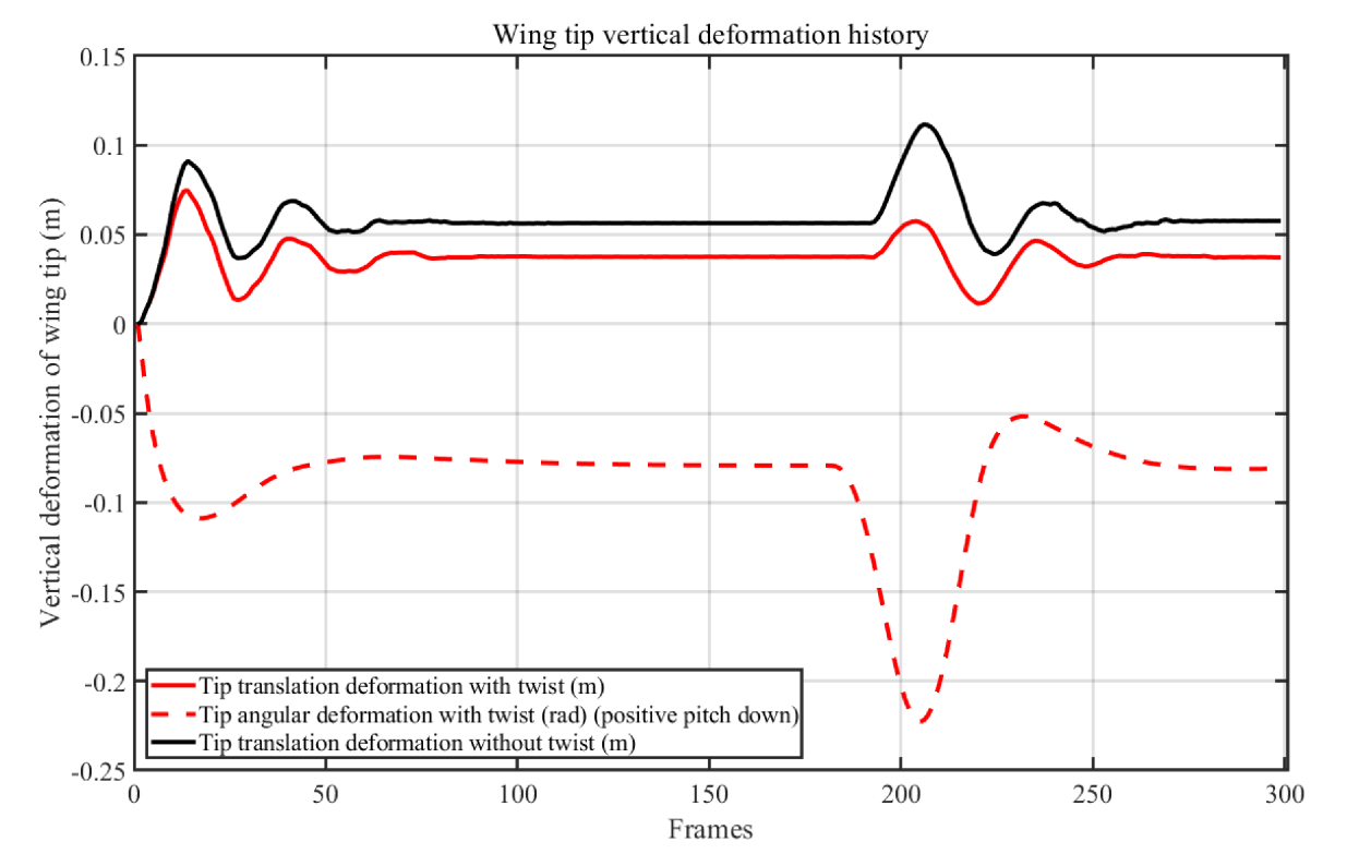
For illustrative purposes, here we present a comparison of wing tip deflection for a generic design showing simulations with and without a twist in Figure A2. These simulations were performed with a value of S = 40 and M = 12 in Equation (37), and the wing encountering the gust centred at frame 200 of the simulation (corresponding to x 0 = 200 ). The coupling of the bending with the twisting in this way will be a topic of our future research.
Figure A2. Prediction of the deformation of an aircraft wing tip with and without twisting.
Aerospace 08 00356 g0a2

References

  1. Gao, S.; Liu, J. Adaptive neural network vibration control of a flexible aircraft wing system with input signal quantization. Aerosp. Sci. Technol. 2020, 96, 105593. [Google Scholar] [CrossRef]
  2. Azimi, M.; Farzaneh Joubaneh, E. Dynamic modeling and vibration control of a coupled rigid-flexible high-order structural system: A comparative study. Aerosp. Sci. Technol. 2020, 102, 105875. [Google Scholar] [CrossRef]
  3. Bekemeyer, P.; Timme, S. Flexible aircraft gust encounter simulation using subspace projection model reduction. Aerosp. Sci. Technol. 2019, 86, 805–817. [Google Scholar] [CrossRef]
  4. Liu, Z.; Liu, J.; He, W. Dynamic modeling and vibration control of a flexible aerial refueling hose. Aerosp. Sci. Technol. 2016, 55, 92–102. [Google Scholar] [CrossRef]
  5. Amoozgar, M.; Fazelzadeh, S.; Haddad Khodaparast, H.; Friswell, M.; Cooper, J. Aeroelastic stability analysis of aircraft wings with initial curvature. Aerosp. Sci. Technol. 2020, 107, 106241. [Google Scholar] [CrossRef]
  6. Vazhayil Thomas, P.; ElSayed, M.S.; Walch, D. Development of high fidelity reduced order hybrid stick model for aircraft dynamic aeroelasticity analysis. Aerosp. Sci. Technol. 2019, 87, 404–416. [Google Scholar] [CrossRef]
  7. Rajpal, D.; Gillebaart, E.; De Breuker, R. Preliminary aeroelastic design of composite wings subjected to critical gust loads. Aerosp. Sci. Technol. 2019, 85, 96–112. [Google Scholar] [CrossRef]
  8. Tsushima, N.; Yokozeki, T.; Su, W.; Arizono, H. Geometrically nonlinear static aeroelastic analysis of composite morphing wing with corrugated structures. Aerosp. Sci. Technol. 2019, 88, 244–257. [Google Scholar] [CrossRef]
  9. Rong, Z.; Cao, B.; Hu, J. Stability analysis on an aeroelastic system for design of a flutter energy harvester. Aerosp. Sci. Technol. 2017, 60, 203–209. [Google Scholar] [CrossRef]
  10. Sommerwerk, K.; Michels, B.; Lindhorst, K.; Haupt, M.; Horst, P. Application of efficient surrogate modeling to aeroelastic analyses of an aircraft wing. Aerosp. Sci. Technol. 2016, 55, 314–323. [Google Scholar] [CrossRef]
  11. Qin, Z.; Marzocca, P.; Librescu, L. Aeroelastic instability and response of advanced aircraft wings at subsonic flight speeds. Aerosp. Sci. Technol. 2002, 6, 195–208. [Google Scholar] [CrossRef]
  12. Timoshenko, S.P. History of Strength of Materials: With a Brief Account of the History of Theory of Elasticity and Theory of Structures; Dover Publications, Inc.: New York, NY, USA, 1983. [Google Scholar]
  13. Murua, J.; Palacios, R.; Graham, J.M.R. Applications of the Unsteady Vortex-Lattice Method in Aircraft Aeroelasticity and Flight Dynamics. Prog. Aerosp. Sci. 2012, 55, 46–72. [Google Scholar] [CrossRef] [Green Version]
  14. Hodges, D.H.; Pierce, G.A. Introduction to Structural Dynamics and Aeroelasticity; Cambridge Aerospace Series; Cambridge University Press: Cambridge, UK, 2002. [Google Scholar]
  15. Wright, J.R.; Cooper, J.E. Introduction to Aircraft Aeroelasticity and Loads; John Wiley and Sons Inc.: Hoboken, NJ, USA, 2007. [Google Scholar]
  16. Bisplinghoff, R.L.; Ashley, H. Principles of Aeroelasticity; Dover Publications Inc.: New York, NY, USA, 2002. [Google Scholar]
  17. Bisplinghoff, R.L.; Ashley, H.; Halfman, R.L. Aeroelasticity; Dover Publications, Inc.: Mineola, NY, USA, 1996. [Google Scholar]
  18. Fernández-Sáeza, J.; Zaeraa, R.; Loyaa, J.A.; Reddy, J.N. Bending of Euler–Bernoulli beams using Eringen’s integral formulation: A paradox resolved. Int. J. Eng. Sci. 2015, 99, 107–116. [Google Scholar] [CrossRef] [Green Version]
  19. Tari, H.; Kinzel, G.L.; Mendelsohn, D.A. Cartesian and piecewise parametric large deflection solutions of tip point loaded Euler–Bernoulli cantilever beams. Int. J. Mech. Sci. 2015, 100, 216–225. [Google Scholar] [CrossRef]
  20. Scuciato, R.; Carrer, J.; Mansur, W. The time-dependent boundary element method formulation applied to dynamic analysis of Euler–Bernoulli beams: The linear theta method. Eng. Anal. Bound. Elem. 2017, 79, 98–109. [Google Scholar] [CrossRef]
  21. Scuciato, R.; Carrer, J.; Mansur, W. Dynamic analysis of Euler–Bernoulli beams by the time-dependent boundary element method formulation. Eng. Anal. Bound. Elem. 2016, 63, 134–153. [Google Scholar] [CrossRef]
  22. Li, F.L.; Sun, Z.Z. A finite difference scheme for solving the Timoshenko beam equations with boundary feedback. J. Comput. Appl. Math. 2007, 200, 606–627. [Google Scholar] [CrossRef] [Green Version]
  23. Kundu, B.; Ganguli, R. Analysis of weak solution of Euler–Bernoulli beam with axial force. Appl. Math. Comput. 2017, 298, 247–260. [Google Scholar] [CrossRef]
  24. Fleischmann, D.; Lone, M.; Weber, S.; Sharma, A. Fast Computational Aeroelastic Analysis of Helicopter Rotor Blades. In Proceedings of the 2018 AIAA Aerospace Sciences Meeting, Kissimmee, FL, USA, 8–12 January 2018. [Google Scholar]
  25. Li, S.R.; Cao, D.F.; Wan, Z.Q. Bending solutions of FGM Timoshenko beams from those of the homogenous Euler–Bernoulli beams. Appl. Math. Model. 2013, 37, 7077–7085. [Google Scholar] [CrossRef]
  26. Yuan, G. Determination of two unknowns simultaneously for stochastic Euler–Bernoulli beam equations. J. Math. Anal. Appl. 2017, 450, 137–151. [Google Scholar] [CrossRef]
  27. Miao, Y.; Shi, Y.; Luo, H.; Gao, R. Closed-form solution considering the tangential effect under harmonic line load for an infinite Euler–Bernoulli beam on elastic foundation. Appl. Math. Model. 2018, 54, 21–33. [Google Scholar] [CrossRef]
  28. Xu, X.J.; Zheng, M.L.; Wang, X.C. On vibrations of nonlocal rods: Boundary conditions, exact solutions and their asymptotics. Int. J. Eng. Sci. 2017, 119, 217–231. [Google Scholar] [CrossRef]
  29. Sumelka, W.; Blaszczyk, T.; Liebold, C. Fractional Euler–Bernoulli beams: Theory, numerical study and experimental validation. Eur. J. Mech. Solids 2015, 54, 243–251. [Google Scholar] [CrossRef] [Green Version]
  30. Baghani, M.; Mohammadi, H.; Haghdabadi, R. An analytical solution for shape-memory-polymer Euler–Bernoulli beams under bending. Int. J. Eng. Sci. 2014, 84, 84–90. [Google Scholar] [CrossRef]
  31. Ma, R.; Gao, C. Nodal solutions of a nonlinear eigenvalue problem of the Euler–Bernoulli equation. J. Math. Anal. Appl. 2012, 387, 1160–1166. [Google Scholar] [CrossRef] [Green Version]
  32. Wei, D.; Liu, Y. Analytic and finite element solutions of the power-law Euler–Bernoulli beams. Finite Elem. Anal. Des. 2012, 52, 31–40. [Google Scholar] [CrossRef] [Green Version]
  33. Ndogmo, J. Equivalence transformations of the Euler–Bernoulli equation. Nonlinear Anal. Real World Appl. 2012, 13, 2172–2177. [Google Scholar] [CrossRef] [Green Version]
  34. Djondjorov, P.A. Invariant Properties of Timoshenko Beam Equations. Int. J. Eng. Sci. 1995, 33, 2103–2114. [Google Scholar] [CrossRef]
  35. Elishakoff, I.; Livshits, D. Some Closed-Form Solutions in Random Vibration of Bernoulli–Euler Beams. Int. J. Eng. Sci. 1984, 22, 1291–1302. [Google Scholar] [CrossRef]
  36. Reddy, J.; El-Borgi, S. Eringen’s nonlocal theories of beams accounting for moderate rotations. Int. J. Eng. Sci. 2014, 82, 159–177. [Google Scholar] [CrossRef]
  37. Sarkar, S.; Reddy, J. Exploring the source of non-locality in the Euler–Bernoulli and Timoshenko beam models. Int. J. Eng. Sci. 2016, 104, 110–115. [Google Scholar] [CrossRef]
  38. Khodabakhshi, P.; Reddy, J. A unified integro-differential nonlocal model. Int. J. Eng. Sci. 2015, 95, 60–75. [Google Scholar] [CrossRef] [Green Version]
  39. Roque, C.; Ferreira, A.; Reddy, J. Analysis of Timoshenko nanobeams with a nonlocal formulation and meshless method. Int. J. Eng. Sci. 2011, 49, 976–984. [Google Scholar] [CrossRef]
  40. Ghayesh, M.H.; Farokhi, H.; Gholipour, A. Oscillations of functionally graded microbeams. Int. J. Eng. Sci. 2017, 110, 35–53. [Google Scholar] [CrossRef]
  41. Demir, Ç.; Civalek, Ö. On the analysis of microbeams. Int. J. Eng. Sci. 2017, 121, 14–33. [Google Scholar] [CrossRef]
  42. Rahaeifard, M. Static behavior of bilayer microcantilevers under thermal actuation. Int. J. Eng. Sci. 2016, 107, 28–35. [Google Scholar] [CrossRef]
  43. Dehrouyeh-Semnani, A.M.; Mostafaei, H.; Nikkhah-Bahrami, M. Free flexural vibration of geometrically imperfect functionally graded microbeams. Int. J. Eng. Sci. 2016, 105, 56–79. [Google Scholar] [CrossRef]
  44. Shafiei, N.; Kazemi, M.; Ghadiri, M. Comparison of modeling of the rotating tapered axially functionally graded Timoshenko and Euler–Bernoulli microbeams. Phys. E 2016, 83, 74–87. [Google Scholar] [CrossRef]
  45. Nejad, M.Z.; Hadi, A. Non-local analysis of free vibration of bi-directional functionally graded Euler–Bernoulli nano-beams. Int. J. Eng. Sci. 2016, 105, 1–11. [Google Scholar] [CrossRef]
  46. Nejad, M.Z.; Hadi, A.; Rastgoo, A. Buckling analysis of arbitrary two-directional functionally graded Euler–Bernoulli nano-beams based on nonlocal elasticity theory. Int. J. Eng. Sci. 2016, 103, 1–10. [Google Scholar] [CrossRef]
  47. Dehrouyeh-Semnaini, A.M.; Nikkhah-Bahrami, M. A discussion on incorporating the Poisson effect in microbeam models based on modified couple stress theory. Int. J. Eng. Sci. 2014, 86, 20–25. [Google Scholar] [CrossRef]
  48. Abadi, M.M.; Daneshmehr, A. An investigation of modified couple stress theory in buckling analysis of micro composite laminated Euler–Bernoulli and Timoshenko beams. Int. J. Eng. Sci. 2014, 75, 40–53. [Google Scholar] [CrossRef]
  49. Dehrouyeh-Semnaini, A.M. A discussion on different non-classical constitutive models of microbeam. Int. J. Eng. Sci. 2014, 85, 66–73. [Google Scholar] [CrossRef]
  50. Eltaher, M.; Alshorbagy, A.E.; Mahmoud, F. Vibration analysis of Euler–Bernoulli nanobeams by using finite element method. Appl. Math. Model. 2013, 37, 4787–4797. [Google Scholar] [CrossRef]
  51. Kong, S.; Zhou, S.; Nie, Z.; Wang, K. Static and dynamic analysis of micro beams based on strain gradient elasticity theory. Int. J. Eng. Sci. 2009, 47, 487–498. [Google Scholar] [CrossRef]
  52. Kong, S.; Zhou, S.; Nie, Z.; Wang, K. The size-dependent natural frequency of Bernoulli–Euler micro-beams. Int. J. Eng. Sci. 2008, 46, 427–437. [Google Scholar] [CrossRef]
  53. Khajeansari, A.; Baradaran, G.; Yvonnet, J. An explicit solution for bending of nanowires lying on Winkler-Pasternak elastic substrate medium based on the Euler–Bernoulli beam theory. Int. J. Eng. Sci. 2012, 52, 115–128. [Google Scholar] [CrossRef]
  54. Giunta, F.; Muscolino, G.; Sofic, A.; Elishakoff, I. Dynamic analysis of Bernoulli–Euler beams with interval uncertainties under moving loads. Procedia Eng. 2017, 199, 2591–2596. [Google Scholar] [CrossRef]
  55. Prasad, B. On the Response of a Timoshenko Beam Under Initial Stress to a Moving Load. Int. J. Eng. Sci. 1981, 19, 615–628. [Google Scholar] [CrossRef]
  56. Shang, H.; Machado, R.; Filho, J.A. Dynamic analysis of Euler–Bernoulli beam problems using the Generalized Finite Element Method. Comput. Struct. 2016, 173, 109–122. [Google Scholar] [CrossRef]
  57. Lerma, A.; Hinestroza, D. Coefficient identification in the Euler–Bernoulli equation using regularization methods. Appl. Math. Model. 2017, 41, 223–235. [Google Scholar] [CrossRef]
  58. Kawano, A. Uniqueness in the determination of unknown coefficients of an Euler–Bernoulli beam equation with observation in an arbitrary small interval of time. J. Math. Anal. Appl. 2017, 452, 351–360. [Google Scholar] [CrossRef]
  59. Marinov, T.T.; Vatsala, A.S. Inverse problem for coefficient identification in the Euler–Bernoulli equation. Comput. Math. Appl. 2008, 56, 400–410. [Google Scholar] [CrossRef] [Green Version]
  60. Marinova, T.T.; Marinova, R.S. Coefficient identification in Euler–Bernoulli equation from over-posed data. J. Comput. Appl. Math. 2010, 235, 450–459. [Google Scholar] [CrossRef] [Green Version]
  61. Ajaj, R.M. Flight dynamics of transport aircraft equipped with flared-hinge folding wingtips. J. Aicraft 2020, 58, 98–110. [Google Scholar] [CrossRef]
  62. Ajaj, R.M.; Saavedra Flores, E.I.; Amoozgar, M.; Cooper, J.E. A Parametric Study on the Aeroelasticity of Flared Hinge Folding Wingtips. Aerospace 2021, 8, 221. [Google Scholar] [CrossRef]
  63. Castrichini, A.; Siddaramaiah, V.; Calderon, D.; Cooper, J.; Wilson, T.; Lemmens, Y. Preliminary investigation of use of flexible folding wing tips for static and dynamic load alleviation. Aeronaut. J. 2017, 121, 73–94. [Google Scholar] [CrossRef] [Green Version]
  64. Balatti, D.; Khodaparast, H.H.; Friswell, M.I.; Manolesos, M.; Amoozgar, M. The effect of folding wingtips on the worst-case gust loads of a simplified aircraft model. J. Aerosp. Eng. Inst. Mech. Eng. 2021. [Google Scholar] [CrossRef]
  65. Iskandarani, D.M. Finite Difference Approximation of Derivatives; Technical Report; Rosenstiel School of Marine Atmospheric Science University of Miami: Miami, FL, USA, 2015. [Google Scholar]
  66. Roache, P.J. Verification and Validation in Computational Sciences and Engineering; Hermosa Publishers: Socorro, NM, USA, 1998. [Google Scholar]
  67. Richtmyer, R.D.; Morton, K.W. Difference Methods for Initial-Value Problems; Krieger Publishing Company: Malabar, FL, USA, 1957. [Google Scholar]
  68. ANM-115. Dynamic Gust Loads; Number 25.341-1 in Advisory Circulars; Federal Aviation Administration: Washington, DC, USA, 2014. [Google Scholar]
  69. Katz, J.; Plotkin, A. Low Speed Aerodynamics; Cambridge University Press: Cambridge, UK, 2001. [Google Scholar]
  70. Belendez, T.; Neipp, C.; Belendez, A. Numerical and Experimental Analysis of a Cantilever Beam: A Laboratory Project to Introduce Geometric Nonlinearity in Mechanics of Materials. Int. J. Eng. Educ. 2003, 19, 885–892. [Google Scholar]
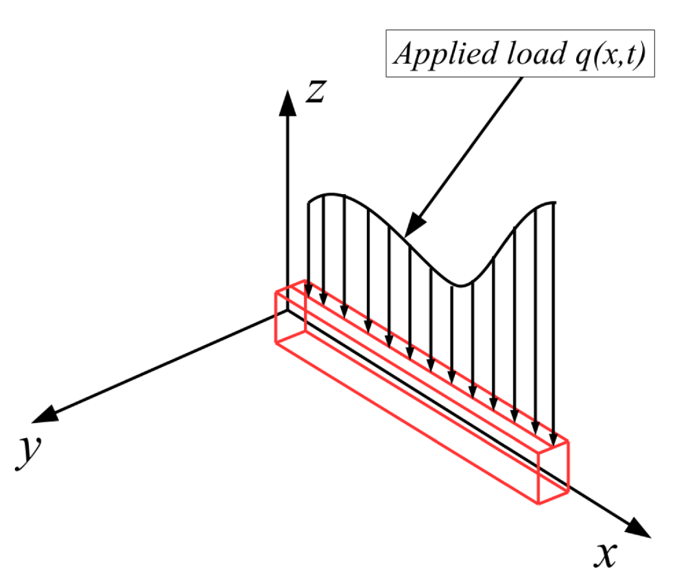
Figure 1. The coordinate system of a structural beam along with the notation used in this paper.
Aerospace 08 00356 g001
Figure 2. The computational domain used in the beam/finite difference simulations.
Aerospace 08 00356 g002
Figure 3. Fourth-order derivative bias stencil for wild oscillatory behaviour.
Aerospace 08 00356 g003
Figure 4. Fourth-order derivative bias stencil for good agreement with physical behaviour.
Aerospace 08 00356 g004
Figure 5. Stencil for the spatial and temporal discretisation of the function w in the finite difference scheme.
Aerospace 08 00356 g005
Figure 6. Stencil for the function F in the finite difference index grid.
Aerospace 08 00356 g006
Figure 7. Beam deformation distributions for the four grid convergence study cases.
Aerospace 08 00356 g007
Figure 8. Analytical solution of the Euler–Bernoulli homogeneous equation for a 10-m cantilevered beam in free vibration.
Aerospace 08 00356 g008
Figure 9. Comparison of the tip deflection between the analytical solution and finite difference predictions for a 10-m cantilevered beam in free vibration.
Aerospace 08 00356 g009
Figure 10. Prediction of the deformation of an aircraft wing.
Aerospace 08 00356 g010
Figure 11. Wing spar model geometry and mechanical properties.
Aerospace 08 00356 g011
Figure 12. Wing spar experimental set-up.
Aerospace 08 00356 g012
Figure 13. Experiment versus simulation.
Aerospace 08 00356 g013
Table 1. Physical parameters used in the grid convergence study of the Euler–Bernoulli finite difference scheme.
SymbolNameVaueUnitsNotes
t -1.0s
EYoung’s modulus 70.0 × 10 9 N/m2Aluminium
ISecond moment of area 6.67 × 10 5 m4Rectangular section, height 0.2 m, breadth 0.1 m
MTotal mass80kgMass evenly distributed over the nodes
β Damping coefficient10
qExternal load4940N/m
CFraction of span0.5
LBeam length10m
Table 2. Grid Convergence Index calculations.
j Δ x j Δ t j No. of Iterations i j w j No. of Nodes
10.833 1.0 × 10 4 1.0 × 10 4 131.004313
20.4 3 × 10 5 3.33 × 10 4 261.188126
30.2 8 × 10 6 1.24 × 10 5 511.260951
40.1 2 × 10 6 5 × 10 5 1011.2957101
Table 3. Second Grid Convergence Index calculations.
j Δ x j Δ t j No. of Iterations i j w j No. of NodesNo. of Oscillations
10.8 1.0 × 10 4 1.0 × 10 4 13−0.7165135
20.4 3 × 10 5 3.33 × 10 4 263.1390264.6
30.2 8 × 10 6 1.24 × 10 5 513.2071514.5
40.1 2 × 10 6 5 × 10 5 1012.57631014.4
Table 4. Wing spar model beam properties.
StationChord Length (m) I y ( m 4 ) Element Mass (kg)
1 100.0000 × 10 3 48.6000 × 10 12 6.8760 × 10 3
2 100.0000 × 10 3 48.6000 × 10 12 11.9109 × 10 3
3 173.2233 × 10 3 84.1865 × 10 12 11.4449 × 10 3
4 166.4466 × 10 3 80.8930 × 10 12 10.9789 × 10 3
5 159.6699 × 10 3 77.5996 × 10 12 10.5130 × 10 3
6 152.8932 × 10 3 74.3061 × 10 12 10.0470 × 10 3
7 146.1165 × 10 3 71.0126 × 10 12 9.5810 × 10 3
8 139.3398 × 10 3 67.7191 × 10 12 9.1151 × 10 3
9 132.5631 × 10 3 64.4256 × 10 12 8.6491 × 10 3
10 125.7864 × 10 3 61.1322 × 10 12 8.1831 × 10 3
11 119.0096 × 10 3 57.8387 × 10 12 7.7172 × 10 3
12 112.2329 × 10 3 54.5452 × 10 12 7.2512 × 10 3
13 105.4562 × 10 3 51.2517 × 10 12 6.7852 × 10 3
14 98.6795 × 10 3 47.9582 × 10 12 6.3193 × 10 3
15 91.9028 × 10 3 44.6648 × 10 12 5.8533 × 10 3
16 85.1261 × 10 3 41.3713 × 10 12 5.3873 × 10 3
17 78.3494 × 10 3 38.0778 × 10 12 4.9214 × 10 3
18 71.5727 × 10 3 34.7843 × 10 12 4.4554 × 10 3
19 64.7960 × 10 3 31.4909 × 10 12 3.9894 × 10 3
20 58.0193 × 10 3 28.1974 × 10 12 3.7958 × 10 3
21 55.2031 × 10 3 26.8287 × 10 12 3.7111 × 10 3
22 53.9721 × 10 3 26.2304 × 10 12 3.6265 × 10 3
23 52.7411 × 10 3 25.6322 × 10 12 3.5419 × 10 3
24 51.5101 × 10 3 25.0339 × 10 12 3.4572 × 10 3
25 50.2791 × 10 3 24.4357 × 10 12 3.3726 × 10 3
26 49.0482 × 10 3 23.8374 × 10 12 3.2879 × 10 3
27 47.8172 × 10 3 23.2391 × 10 12 3.2033 × 10 3
28 46.5862 × 10 3 22.6409 × 10 12 3.1186 × 10 3
29 45.3552 × 10 3 22.0426 × 10 12 3.0340 × 10 3
30 44.1242 × 10 3 21.4444 × 10 12 2.9494 × 10 3
31 42.8932 × 10 3 20.8461 × 10 12 2.8647 × 10 3
32 41.6623 × 10 3 20.2479 × 10 12 2.7801 × 10 3
33 40.4313 × 10 3 19.6496 × 10 12 2.6954 × 10 3
34 39.2003 × 10 3 19.0513 × 10 12 2.6108 × 10 3
35 37.9693 × 10 3 18.4531 × 10 12 2.5261 × 10 3
36 36.7383 × 10 3 17.8548 × 10 12 2.4415 × 10 3
37 35.5073 × 10 3 17.2566 × 10 12 2.3569 × 10 3
38 34.2764 × 10 3 16.6583 × 10 12 2.2722 × 10 3
39 33.0454 × 10 3 16.0601 × 10 12 2.1876 × 10 3
40 31.8144 × 10 3 15.4618 × 10 12 2.1029 × 10 3
41 30.5834 × 10 3 14.8635 × 10 12 2.0183 × 10 3
42 29.3524 × 10 3 14.2653 × 10 12 1.9336 × 10 3
43 28.1214 × 10 3 13.6670 × 10 12 1.8490 × 10 3
44 26.8905 × 10 3 13.0688 × 10 12 1.7644 × 10 3
45 25.6595 × 10 3 12.4705 × 10 12 1.6797 × 10 3
46 24.4285 × 10 3 11.8722 × 10 12 1.5951 × 10 3
47 23.1975 × 10 3 11.2740 × 10 12 1.5104 × 10 3
48 21.9665 × 10 3 10.6757 × 10 12 1.4258 × 10 3
49 20.7355 × 10 3 10.0775 × 10 12 1.3411 × 10 3
50 19.5046 × 10 3 9.4792 × 10 12 1.2565 × 10 3
51 18.2736 × 10 3 8.8810 × 10 12 1.1719 × 10 3
52 17.0426 × 10 3 8.2827 × 10 12 -
Table 5. Comparison between measured and predicted deflections for the wing spar experiment.
CaseTip Load (N)Measured Deflection (m)Simulated Deflection.
Thickness 1.9 mm
Simulated Deflection.
Thickness 1.8 mm
Simulated Deflection.
Thickness 1.6 mm
00.0000.0260.01350.01500.024
10.0980.0290.01510.01690.027
20.1960.0330.01680.01890.031
30.2940.0360.01840.02080.035
40.3920.0390.02000.02270.038
50.4900.0420.02170.02460.042
60.6870.0480.02490.02850.050
70.9810.0560.02990.03430.061
81.1770.0620.03310.03810.068
91.3730.0690.03640.04200.076
101.4710.0710.03810.04390.079
111.6680.0760.04130.04780.087
121.9620.0860.04630.05360.097
Publisher’s Note: MDPI stays neutral with regard to jurisdictional claims in published maps and institutional affiliations.