Article

Physics Guided Deep Learning for Data-Driven Aircraft Fuel Consumption Modeling

1
Faculty of Aeronautics and Astronautics, Istanbul Technical University, Istanbul 34469, Turkey
2
Digital Transformation Office, Presidency of the Republic of Turkey, Ankara 06550, Turkey
3
Centre for Autonomous & Cyber-Physical Systems, School of Aerospace, Transport and Manufacturing, Cranfield University, Cranfield MK43 0AL, UK
*
Author to whom correspondence should be addressed.
Aerospace 2021, 8(2), 44; https://doi.org/10.3390/aerospace8020044
Submission received: 3 January 2021 / Revised: 22 January 2021 / Accepted: 4 February 2021 / Published: 8 February 2021
(This article belongs to the Special Issue Aeronautical Informatics)

Abstract

:
This paper presents a physics-guided deep neural network framework to estimate fuel consumption of an aircraft. The framework aims to improve data-driven models’ consistency in flight regimes that are not covered by data. In particular, we guide the neural network with the equations that represent fuel flow dynamics. In addition to the empirical error, we embed this physical knowledge as several extra loss terms. Results show that our proposed model accomplishes correct predictions on the labeled test set, as well as assuring physical consistency in unseen flight regimes. The results indicate that our model, while being applicable to the aircraft’s complete flight envelope, yields lower fuel consumption error measures compared to the model-based approaches and other supervised learning techniques utilizing the same training data sets. In addition, our deep learning model produces fuel consumption trends similar to the BADA4 aircraft performance model, which is widely utilized in real-world operations, in unseen and untrained flight regimes. In contrast, the other supervised learning techniques fail to produce meaningful results. Overall, the proposed methodology enhances the explainability of data-driven models without deteriorating accuracy.

1. Introduction

Physical modelling, such as aircraft fuel consumption modeling, is used extensively to design and to predict processes in a wide range of engineering applications including flight planning [1,2]. Although the underlying flight dynamic models are based on physical principles and physical laws, these are approximations of actual processes with added errors and biases based on a series of underlying assumptions and simplifications [3,4,5]. In addition, these models also contain a number of parameters, the values of which have to be calculated with scarce observed data, further decreasing their accuracy, largely due to the variability of the underlying physical-rules in both space and time [6].
Machine Learning (ML) algorithms have been shown to produce models that capture actual physical processes in a wide range of engineering disciplines including aircraft performance modeling [7,8]. In that aspect, the most critical aspect in such flight performance modeling is to extract the actual fuel usage based on the flying conditions such as Mach number, altitude number and environmental conditions including disturbances such as wind [9]. As such, ML algorithms, are shown to be able to automatically extract complicated relationships from data [10]. A significant deduction for this conclusion is that ML models, given sufficient data, can find formation and patterns in data where the underlying complexity prevents the precise physics-based modeling of a system’s actual process characteristics. However, the validity of such ML driven models across the whole operational state-space (in this case the whole flight envelope) is complicated by a few critical factors [11]. In particular, even though state-of-the-art ML models can seize entangled spatial-temporal correlations and relations, they require a vast amount of labeled data for training and testing, seldom available in real applications. [12] In addition to this, ML algorithms and methods often give scientifically discrepant results. They can only effectively capture relations in the possible training data and hence have a poor out-of-sample generalization capability [13,14,15]. This is indeed a fact which is also valid for the fuel burn modeling of an aircraft [16].
Recently, with the appearance of novel deep learning algorithms, there has been an interest in using operational flight data recorded by aircraft for several purposes. One of the significant applications is to improve fuel consumption predictions for given atmospheric and flight conditions, and thus to have higher precision flight performance models for optimized flight planning. Conventional supervised machine learning algorithms perform well on this problem, but their applicability is limited by the flight envelope available within the training data. A black-box fuel consumption model ensures coherent outputs only for the flight regimes that the data incorporates. In this work, we design a novel physics guided machine learning process for such data-driven aircraft fuel consumption modeling. Specifically, we guide and design the underlying neural networks with the actual physic laws that govern the fuel consumption dynamics. Even though conventional supervised learning algorithms perform well on this problem, we show that their applicability is limited by the actual flight envelope of the underlying training data. With this approach, we show that we improve consistency in unseen flight regimes, thus extending the validity of the machine learning model to the whole flight envelope. To the best of our knowledge, this is the first work that successfully designs and demonstrates a physics-guided deep learning framework in fuel consumption modeling for an aircraft.
In order to obtain more accurate results and reliable out-of-sample generalization, the vital intention is to merge physics-based models with ML algorithms to leverage their complementary capabilities. Such combined ML-physics models are expected to thoroughly seize the dynamics of scientific systems and improve the knowledge of underlying physical laws [17]. There are several ways to inject physical laws, knowledge, or information into ML models to build physics aware ML models [18]. But physical information often shows a high degree of complexity due to connections among many physical variables diversifying over space and time at various ranges [19]. Conventional ML models can fall short of directly obtaining such relations from data, primarily when given limited measurement data [20]. This scarce data problem is one cause for the failure of the generalization to the circumstances in unseen training data. As a result, several novel research has been used to include physical information into training loss functions to support ML models to seize generalizable patterns consistent with underlying physical laws and governing equations. One of the most common ways to make machine learning models consistent with physical laws is by extending the loss function of the machine learning models to include physical constraints and other physical information [21]. Although the concept of integrating scientific knowledge and machine learning models has only become a popular topic of scientific research in the last few years, there is already extensive literature on this topic [22,23,24]. In the last decade, there has been an increase in utilizing operational flight data, namely Quick Access Recorder (QAR) or Flight Data Recorder (FDR) [25] for many applications such as performance monitoring, anomaly detection, or weather forecasting [26,27,28,29]. These data consist of historical logs of all parameters that can be measured or observed through on-board sensors and systems. Even though they do not have information on the thrust, drag or lift, they record critical performance indicators such as vertical speed, gross weight and fuel flow. This capability makes them highly suitable for the supervised learning of aircraft performance. Chati and Balakrishnan used FDR data in tree-based learning and Gaussian process algorithms to model fuel flow [16,30,31]. Baklacioglu [32] combined genetic algorithms and neural networks for the same purpose. Baumann and Klingauf [10] proposed another scheme for supervised learning of fuel consumption with FDR. The works of Huang et al. [33] and Khadilkar [34] are other examples that have used operational data. These studies proved that aircraft performance can be represented through machine learning techniques. However, they did not investigate model performances in flight regimes that are not covered by the training data. Thus, the applicability of the proposed approaches to the complete flight envelope remains an open issue.
This paper derives from our previous study on tail-specific fuel consumption modeling [7]. Previously, we proved that using proper neural network architectures and hyper-parameters, it is possible to build satisfactory fuel consumption models capturing actual profiles. The simplicity in fuel consumption modeling is that the parameters it depends on are distinct. In a nutshell, fuel consumption varies with the amount of thrust to be produced, altitude, and Mach number. However, the inter-dependencies are non-linear and complex. As illustrated in our previous work, deep neural networks are very efficient for this problem because neural networks can be used as universal function approximation under certain conditions [16,35]. However, extrapolating to the flight or atmospheric conditions that are not in the data is challenging and out-of-distribution generalization capability of neural network models or even any machine learning algorithms may not be enough to approximate the latent or hidden functions related to problem. Granted that the data comprehend samples from operational limit conditions, a black-box model could be extrapolated to some degree. However, it is not the case in real operations because the regimes aircraft fly are determined by either air traffic regulations or airline preferences. Moreover, in a level flight, aircraft speed (Mach number) is set to a fixed value, and altitude is constant. Commercial aircraft usually cruise at altitudes proportional to one thousand feet. Therefore, even though the data cover all cruise levels, there would still be a lack of altitude variance. For instance, operational data of an aircraft with a maximum operable altitude of forty-thousand feet would have forty-one distinct altitudes at best. The case with the Mach number is even more challenging, because the most efficient Mach speeds for jet aircraft usually converge to a very narrow region at high altitudes. For example, narrow-body aircraft generally cruise at 0.78 Mach, whereas wide-body aircraft fly 0.83 [36]. Additionally, airlines prefer high altitude cruise for fuel-efficiency. Therefore, the Mach number variation observed in operational data is limited.
This paper aims to overcome this problem by introducing the cruise fuel flow dynamics into the deep neural networks. First, we analyze the model-based approaches and data to identify a physical intuition that we can embed as a criterion. Then, we generate artificial data-sets that the operational data do not cover. We train our deep neural network such that it learns a mapping for fuel consumption from the labeled data, and captures the physics-guidance we introduce through unlabeled artificial data. This paper’s contributions are: First, we select a physical-guidance function that is valid for all feasible flight conditions. Second, our methodology can be implemented for any parameter that lacks variation in data. Last, our framework produces physically-consistent outputs for unseen flight regimes.
The remainder of this manuscript is organized as follows: Section 2 provides a generic description of the problem. Section 3 is dedicated to describe technical background on neural networks, and fuel consumption dynamics in cruise flight. In Section 4, we explain our methodology for developing the physical-guidance for fuel consumption, and how to embed it into the neural networks. Section 5 demonstrates the results for a wide-body aircraft. Finally, Section 6 concludes the paper, and discusses open issues as well as the future work.

2. Problem Formulation

We are interested in estimating fuel consumption from engines for a complete flight envelope. The aim is to find the fuel consumption estimator f F F : X Y , where X is the set of inputs, and Y is the target variable, which is fuel consumption from engines in mass per time. We aim to find a proper function approximation such that:
f F F X = Y ^
f F F = arg min f J E Y , Y ^ + λ S J S f + λ P H Y J P H Y ( Y ^ )
where Y ^ is the predicted fuel consumption, J E is the empirical error, and J S is the model complexity (regularization term). Considering only J E and J S is the formulation of a generic supervised learning problem. However, a model trained in this scheme does not assure physically consistent fuel consumption predictions or known-physical laws for the complete state space. Hence, we introduce the physical inconsistency loss denoted by J P H Y . It quantifies how physical laws, constraints or relationships are violated, provides physical intuition and knowledge for the model to improve generalization capability. We can define these as:
g X , Y , d Y d X , d Y d t , d 2 Y d X 2 , = 0
h X , Y , d Y d X , d Y d t , d 2 Y d X 2 , 0
In Equations (3) and (4), g and h are known or derivable functions to express the physical constraints, laws or relations. By using these type of equations or inequalities, additional physics based knowledge can be injected in to ML model to learn by introducing an additional physical inconsistency loss.
The physical inconsistency loss J P H Y penalizes model predictions that contravene these constraints. Finally, the hyper-parameters λ ( . ) are the coefficients of physical loss components contributing to the penalization of the loss, related to specific physical-knowledge or law. By adjusting coefficients of these terms, level of the involvement of the physical laws or knowledge of the system can be adjusted to the machine learning model. Obtaining the values of λ ( . ) coefficients is generally possible with experimentally or trial-and-error methods. Adjusting these values provides the injection degree of the physical intuition into ML model. The function approximation process is illustrated in Figure 1. Inputs to the neural network are features related to problem, labeled data, and unlabeled data in which we have knowledge of fuel consumption behavior. One contributor to the main loss function is the empirical error, where we measure how accurate the model is at predicting fuel consumption. As for the unlabeled data, even though we cannot measure any prediction error, we can check whether the output satisfies some physical constraints such as positiveness, monotonic increase/decrease, convexity or physical conservation laws [37]. The most crucial point is that all the terms in the loss function have to be differentiable to calculate gradients with respect to the model parameters. One way of expressing and implementing the constraints in a loss function is to use well-known activation functions such as ReLU, ELU, TanH, and Sigmoid. These activation functions’ differentiability property helps to build a strong framework to express the physical constraints and information.
Combining all the required loss terms that include physical knowledge and constraints, the final loss function can be used for the optimization of the model parameters by using convex or other heuristic optimization techniques. However, one important issue must be noted that even though using this type of implementation has several advantages, the most crucial drawback would be making the loss function more complex. As a result, the optimization of the model parameters with the physics-based loss function can eventually be complicated, and thus leading to longer convergence time in the training of the model. As such, convergence to local optimal solutions during training is possible. To solve these problems, second order optimization algorithms such as Limited Memory Broyden–Fletcher–Goldfarb–Shanno (LBFGS) algorithm [38] or usage of combination of different optimization algorithms sequentially and complementary manner can be utilized [39,40].

3. Preliminaries

In this section, we first provide neural network’s Multi-Layer Perceptron (MLP) architecture and its mathematical background as a universal function approximator for regression problems, and then describe the flight physics governing fuel consumption dynamics.

3.1. Neural Networks with Multi-Layer Perceptrons (MLP)

We adopt a fundamental multi-layer perceptron architecture to regress the fuel consumption, Y, using X. For a fully-connected network with L hidden layers, this amounts to the following modeling equations relating the input features x, to its target prediction y.
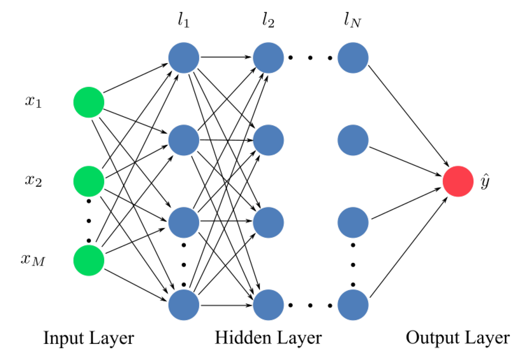
To find the nonlinear mapping for the correction factor τ , we utilize deep neural networks, which have been proven to capture complex input-output relationships through gradient-based optimization and can be used to model any continuous function [41,42]. A generic structure of a deep neural network consisting of a multilayer perceptron with M input features and N layers is illustrated in Figure 2. It is composed of sequentially connected layers, which comprise sets of neurons that are combinations of mathematical operations followed by nonlinear activation functions. The model parameters ξ are defined as ξ = { W , b } , where W = { w i } i = 1 N , and b = { b i } i = 1 N . The output of the lth layer is:
f F F ( x , ξ l ) = f w l , b l ( x ) = z l j = 1 N l w l j x j + b l
= Z l w l T x l + b l ( l = 1 , , N )
where N t is the neuron number and Z l is a nonlinear activation function of a specific lth layer, and x l is the input of the lth layer and also the output of the ( l 1 ) th layer. In addition to this, w l and b l are learnable parameters and called weight and bias terms of that layer respectively. The output of the last layer is a result of the composite and complex mapping defined as:
y ^ ( x ) : =   f w n , b n f w 1 , b 1 ( x )
Back-propagation algorithm [43] is used to train the neural network by utilizing gradient based optimization methods using the loss function given in Equation (8):
f F F = arg min ξ J E Y , Y ^ + λ s J s ξ
To prevent overfitting and improve generalization capability of the neural network, an additional regularization term can be applied to the total loss function in Equation (8). Either L 1 , or L 2 norm penalties, which is also the model complexity loss are given in Equations (9) and (10):
J s ( ξ ) = J s L 1 ( w ) = w 1 = w 1 + w 2 + + w N
J s ( ξ ) = J s L 2 ( w ) = w 2 2 = w 1 2 + w 2 2 + + w n 2
and can be used to regularize the model. The L 1 regularization applies an L 1 norm penalty equal to the absolute value of the coefficient scale. It restricts the scale of the coefficients. L 1 may generate sparse models with few parameters, and specific coefficients may become zero and be discarded. L 2 regularization applies an L 2 penalty equal to the scale square of the coefficients. L 2 can not generate sparse models, and all coefficients are reduced by the same factor. Other regularization methods such as Dropout [44] may help preventing the overfitting for neural networks.

3.2. Cruise Fuel Consumption Dynamics

To understand the parameters affecting fuel consumption, we first need a thrust analysis. The analysis in this section are based on model-based approaches in BADA4 [45], which leverages OEM performance models of Airbus [46] and Boeing [47]. Developers of BADA4 showed the good approximation to these reference models [48]. The cruise phase of a flight is considered to be the equilibrium of both lateral and vertical forces:
L = W
T h = D
where L is the lift, D is the drag, W is the aircraft weight, and T h is the thrust. Equation (12) denotes that thrust required is the drag, and equals to the following aerodynamic equation:
T h r e q = D = 1 2 δ p 0 κ S M 2 C D
where δ is the pressure ratio, p 0 = 101,325 [N/m 2 ] is the air pressure at the sea level, κ = 1.4 is the adiabatic index, M is the Mach number, and C D is the drag coefficient. The drag coefficient is defined as:
C D = C 0 + C 2 C L 2
where C 0 is the skin friction and pressure combined, and C 2 is the lift induced drag coefficients. Thrust produced by the engines is a function of pressure ratio δ , Mach number M, and throttle setting δ T :
T h = f δ , M , δ T
Combining Equations (11) and (13), we can formulate the thrust required in cruise as:
T h r e q = f δ , M , δ T , W
The throttle setting δ T is also referred to RPM or N1. They all determine low-pressure spool speed, which proportionally affects how much fuel is injected into the combustion chamber. In cruise, autopilot systems adjust this parameter to maintain the equilibrium in Equation (13). As seen in Equation (13), pressure ratio dependency is considered to be proportional. Therefore, the nonlinearities are due to Mach number and aircraft mass. Figure 3 illustrates Mach sensitivity of thrust required for selected altitude and mass values. The graphs show higher amounts of thrust required at lower altitudes due to higher density, which results in higher profile drag. Higher air density would also reduce the angle of attack to maintain the same Mach number, hence decreasing the lift coefficient thereby the drag coefficient. However, in this situation, higher density becomes the dominant factor in the thrust required. This can also be directly observed following the parabolic drag polar in which increased density results in the the profile drag dominating the induced drag part. As such, higher aircraft weight results in higher drag due to drag-polar. Transition from thrust to fuel consumption is called thrust specific fuel consumption. Simplified analyses assume it to be constant at each flight level. However, a correction for the Mach number should also be considered because airspeed at the engine inlets affects the engine dynamics, as well. In summary, fuel consumption denoted as F is a function of thrust, Mach number, and altitude. Dependence on altitude is considered to be proportional to the pressure ratio and the square root of temperature ratio. This is shown through dimensional analysis and verified by experimental results [49]. We can formulate fuel consumption F as:
F = δ θ T h M , δ T
In the predecessor of BADA4, namely BADA3 [50], this is modeled as:
F = C f 1 1 + M θ C f 2 T h
where the coefficients C f 1 , 2 are customized to aircraft family. BADA4 fits high-order polynomials to the synthetic data generated from OEM performance models:
F = δ θ p q a p q T h δ q M p
where a p q are the polynomial coefficients, similarly tailored to aircraft types. Equations (17)–(19) are widely utilized real world applications. Figure 4 illustrates fuel flow sensitivity to Mach number for the same conditions presented for thrust analysis. It is not clear to have a generalized statement about the Mach number effect. At high Mach numbers, fuel flow tends to increase. However, it is the opposite at low Mach cruises. As the altitude increases, the minimum Mach number would increase to compensate for lift loss due to decreased air density. This stands for high Mach number cruises at higher altitudes. However, it cannot be generalized to all conditions.
In summary, model-based approaches acknowledge five parameters that alter fuel consumption: (i) pressure ratio δ : appears as a proportional component for constant temperature, mass, and Mach number. (ii) temperature ratio θ : in analytical expressions, fuel consumption is proportional to the square root of the temperature ratio. As side effects, it determines the speed of sound and Mach number, and lower ambient temperatures allow the engine to operate at higher throttle settings [51]. Additionally, a higher atmospheric temperature causes an increase in drag by elevating the Reynolds number. (iii) throttle setting δ T : an increasing throttle consistently escalates fuel flow injected to the fuel chamber. Note that, autopilot system computes the throttle position. Furthermore, how much is should be set depends on how much thrust to be produced. In cruise, this is also a function of aircraft mass because thrust required is drag. (iv) Mach numberM: the Mach number effect on fuel consumption is a combination of its impact on drag, and thrust. Equation (13) reveals a proportional increase in drag with M 2 . Coupled with the impact on thrust, fuel consumption for given pressure ratio δ , temperature ratio θ , and aircraft mass m with increasing Mach number M results in a convex curve.
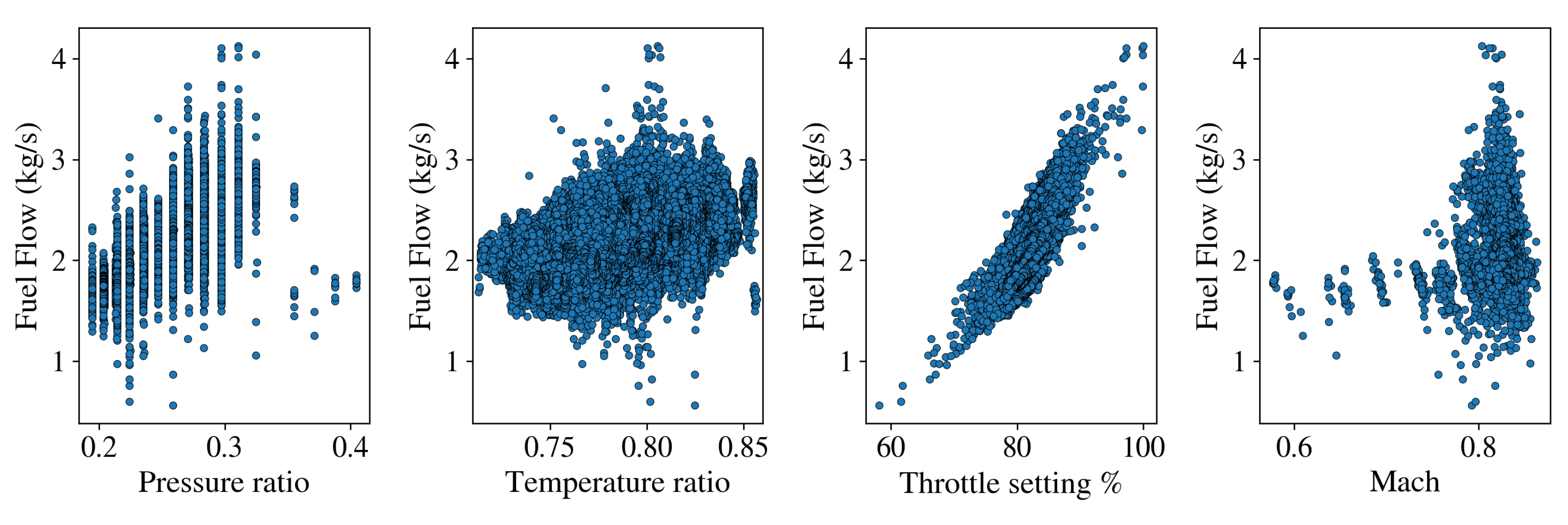
The dynamics described until here were model-based approaches utilized in real-world operations. Figure 5 illustrates how the data present these correlations. They are the results of the combination of all factors. The monotonic relationships with pressure ratio, temperature ratio, and throttle setting are noticeable. However, the Mach number dependency is not clear. Moreover, it is not possible to filter the data for unique aircraft masses and have measurements for every possible Mach number like illustrated in Figure 4. As expected, aircraft operationally had flown only a small subset of the whole flight envelope. The Mach number distribution is skewed, and most of the population is around 0.83, which is usually the nominal cruise speed regime for this aircraft.
For a greater gross weight, an autopilot system sets throttle to a higher position to maintain Equation (12). Figure 6 depicts gross weight correlation with the throttle δ T , and fuel consumption from data. Higher aircraft masses result in higher throttle settings and higher fuel flows.
Finally, Table 1 summarizes parameters in the model-based approaches and QAR data that significantly affect fuel consumption. Statistical significance in the data is computed by Spearman rank, which measures the monotonic relations. Mach number is not in the list for the data because it does not have an acceptable variance. Instead, true airspeed appears, but it is the Mach number corrected with temperature ratio:
V = 340.26 M θ
Hence, the true airspeed’s statistical significance is mostly due to the variation of altitude. This is the main issue with the operational data because even though the Mach number is an important parameter, it does not appear like one. The next section describes how we use fuel consumption dynamics to define a physics-based loss function and implement it into the ML framework.

4. Methodology

This section explains the physical guidance extracted from the fuel consumption analysis and how we implement it into the machine learning framework. First, we derive physics-based loss terms as a guide to the neural network design to capture the underlying physical trends in addition to the data-based correlations. Second, we explain how the physics-based loss terms are integrated through unlabeled artificial data.

4.1. Physics-Based Loss Function Design for Fuel Consumption

In this part of the study, we seek for a physical relationship for fuel flow that satisfies Equations (3) and (4). Equaling a physical quantity to zero is one of the possible approaches, e.g., Typical conservation of mass, conservation of momentum or energy equations with dissipating terms geared towards modeling cumulative effects such as total fuel consumption over distance time. However, we aim to model instantaneous fuel flow given flight and atmospheric conditions. Therefore, we base our approach on intuitive, instantaneous relationships, namely fuel flow’s monotonic increase, and increasing power. It is important to note that the main aim here is to derive a representative equation for the power without utilizing BADA or OEM models. This enables our proposed model to be self-governing, i.e., independent from external performance models and parameters. Starting with the physical principle that
F T h r e q M
and using the Mach - true airspeed formula in Equations (20) and (21) can be written as,
F = λ T h r e q V θ
where the nominator part T r e q V is the required power. The sole variable in the denominator is the temperature. In purely physical terms, given ambient conditions, increasing the power requires more fuel to be injected to the air flow. Hence, fuel flow also increases to maintain the new power setting.
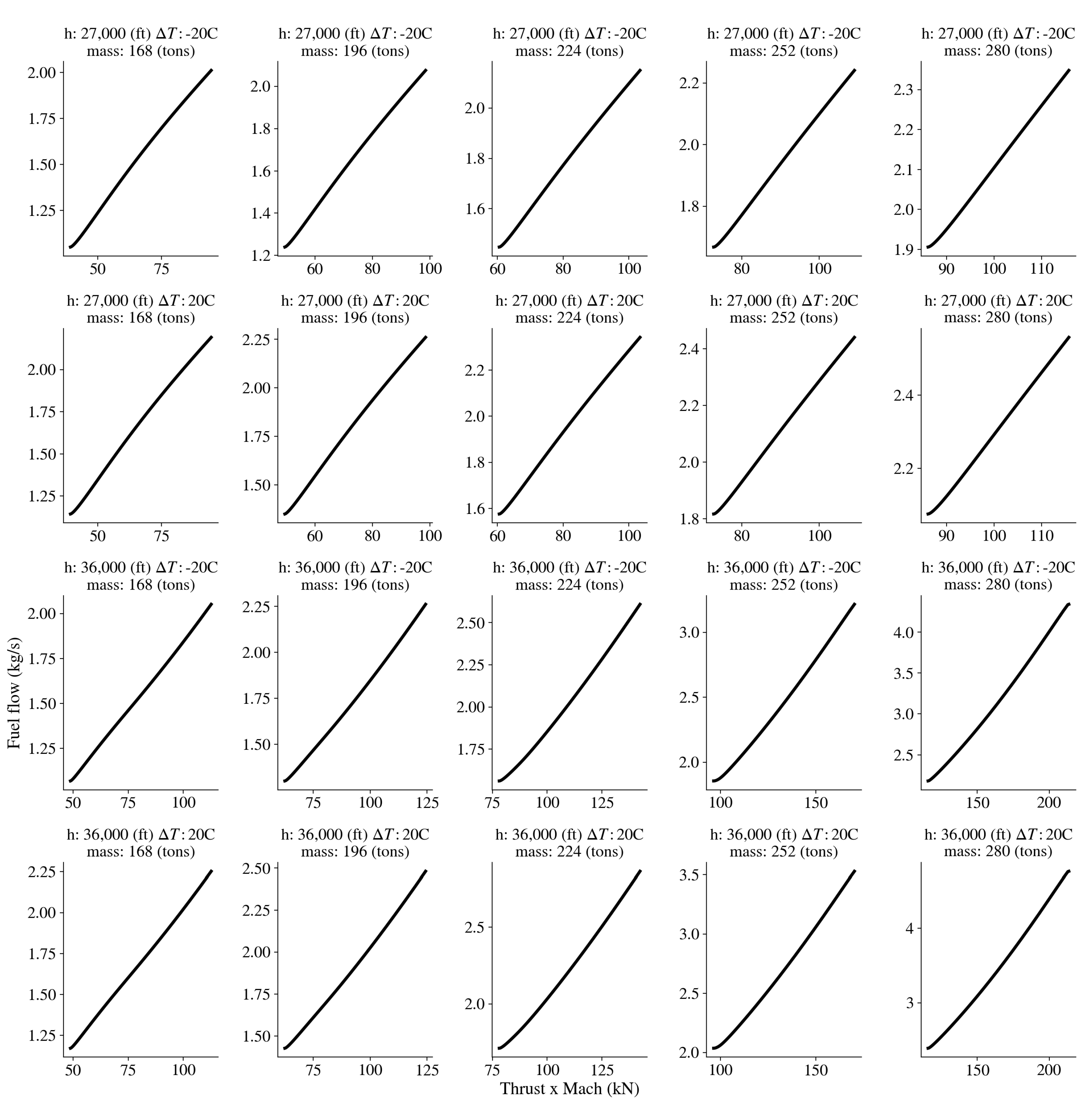
We validate Equation (21) through BADA4. Figure 7 depicts fuel flow with growing T h r e q M term in cruise, given several flight conditions. Note that these are BADA4 model outputs, as well as Boeing’s performance model’s. Each subplot comprises Mach sensitivity similar to thrust and fuel consumption analyses in Section 3. All flight conditions yield increasing fuel flow profiles with increasing T h r e q M . For the rest of the section, we approximate T h r e q M through empirical equations. First, we use the generic drag polar in Equation (14) to approximate the drag coefficient. The thrust required becomes;
T h r e q = c 0 δ M 2 C 0 + C 2 C L 2
where c 0 = 0.5 κ p 0 S . Because all regimes show linear tendencies, we can consider fuel consumption as a multiplication of thrust times Mach with a scalar λ :
F = λ T h r e q M
F = λ c 0 δ M 3 C 0 + C 2 C L 2
As seen in Figure 7, the scalar λ is not always constant. The slope is different at each atmospheric condition—mass combination:
λ = f δ , θ , m
Because the dependency on the mass is only due to drag polar, we can assume λ as a function of pressure and temperature ratios:
λ = f δ , θ
We can consider the scalar λ as a ratio between a constant scalar λ ¯ , and pressure ratio multiplied by square root of temperature ratio. This assumption is based on Equation (17).
λ = λ ¯ δ θ
Similar to the drag equation, the lift equation is:
L = c 0 δ M 2 C L
where lift equals weight in cruise. Hence, the lift coefficient can be calculated as:
C L = W c 0 δ M 2
Finally, combining all equations above, the generalized fuel consumption equation is found as:
T = M θ c 1 M 2 + c 2 m 2 δ 2 M 2
where c 1 = C 0 c 0 and c 2 = C 2 / c 0 are constants, and customized to the aircraft type. We utilize this generalized fuel consumption equation as the primary physical guide to fuel usage for various cruise flight and environmental conditions.

4.2. Implementation of the Physics Guided Loss Function

To generate physical guidance through loss functions, we first generate N e sets consisting of several flight and atmospheric conditions as illustrated in Figure 7. The set is denoted as R = { r n R N r × M r } n = 1 N e , where M r is the number of features, and N r is the number columns in r n . Columns of each set r n are the input features; pressure ratio δ , temperature ratio θ , Mach number M, and aircraft mass m a c . The formulation to generate these sets is to keep parameters constant, except the Mach number M:
r n = δ n θ n M n m i n m a c , n δ n θ n M n m i n + Δ M m a c , n δ n θ n M n m i n + 2 Δ M m a c , n δ n θ n M n m a x m a c , n
where M m i n n and M m a x n are the minimum and maximum operable Mach speeds at the nth set given as { δ n , θ n , m a c , n } . The thrust times Mach set associated to this set r n is denoted by T n = { t m n [ i ] } i = 1 N r . It is calculated through Equation (31), given ith row of r n :
t m n [ i ] = M n [ i ] θ n [ i ] c 1 ( M n [ i ] ) 2 + c 2 ( m a c , n [ i ] ) 2 ( δ n [ i ] ) 2 ( M n [ i ] ) 2
Then, we re-order the associated thrust times Mach such that it monotonically increases:
T n = { t m n [ i ] : t m n [ i + 1 ] t m n [ i ] 0 }
Using the index order in T n , we organize the matrix r n in the same way. The new version is r n :
r n = { r n [ i ] : T ( r n [ i + 1 ] ) > T ( r n [ i ] ) }
Fuel consumption predicted by the model for given r n is Y ^ n , where Y ^ n = f F F ( r n , ξ ) = { y ^ n [ i ] } i = 1 N b . Considering the monotonic increase relationship illustrated in Figure 7, we expect Y ^ n to be in an increasing order. To model this, we divide the predicted fuel consumption Y ^ into two parts as below:
Y ^ n + = { y ^ n [ 2 ] , y ^ n [ 3 ] , , y ^ n [ N b ] }
Y ^ n = { y ^ n [ 1 ] , y ^ n [ 2 ] , , y ^ n [ N b 1 ] }
If the model satisfies the physical laws, element-wise subtraction of Y ^ n from Y ^ n + should always be positive. Hence, we penalize model predictions that violate it. The most practical way to do it is applying ReLU activation function, which is defined as:
R e L U ( x ) = 0 , x < 0 x , x 0
Hence, the first physical loss function related to the monotonicity can be written as:
J P H Y , 1 = 1 N e n = 1 N e i = 1 N r 1 1 N r + R e L U y ^ n [ i ] y ^ n [ i + 1 ]
where N r + stands for the number of positive outputs of R e L U ( x ) , and N b + N r . Previous studies usually divide the sum by N b . However, in our case using such approach causes the loss function to be so small. Therefore it becomes negligible compared to the empirical error. The second physics-guided loss prevents model to predict negative fuel flows, and is defined as:
J P H Y , 2 = 1 N e 1 N r n = 1 N e i = 1 N r R e L U y ^ n [ i ]
The last physics-based loss function is a heuristic limitation to the fuel consumption the model predicts. We limit the difference between the maximum and minimum fuel consumption for a given set of r n with a pre-defined value, denoted by F r e f . Its magnitude hinges on domain expertise from pilots and aircraft performance engineers.
J P H Y , 3 = 1 N e n = 1 N e R e L U max Y ^ n min Y ^ n F r e f
The last two physics-guided losses are more like modifications to the first one. The first intuition enables the model to capture a linear relationship for fuel flow, but it does not include lower and upper limits. That is where the remaining loss terms appear. Finally, the combined physical loss function is the sum of Equations (39)–(41):
J P H Y = i λ P H Y i J P H Y , i
Combined with the empirical error, which is the mean squared error in this study, the final loss function is given in Equation (43):
J = λ e 1 N d i = 1 N d y ^ d [ i ] y d [ i ] 2 + λ s | | W | | 2 2 + 1 N e n = 1 N e i = 1 N r 1 1 N r + R e L U y ^ n [ i ] y ^ n [ i + 1 ] + 1 N e 1 N r n = 1 N e i = 1 N r R e L U y ^ n [ i ] + 1 N e n = 1 N e R e L U max Y ^ n min Y ^ n F r e f
This loss function becomes the main learning function in data-driven neural network design process. In particular, this specific design allows us to capture data correlations and nonlinear relationships inline with the general physical principles that extend beyond the flight envelope as captured by data. In the next section, we demonstrate this methodology by using actual Quick Access Recorder (QAR) data set from a major European flag carrier airline. The results show that the proposed approach allows us to develop more precise fuel consumption (and thus flight performance models) over a wide range of the flight envelope in comparison to standard supervised learning approaches and existing BADA4 model.

5. Experiment

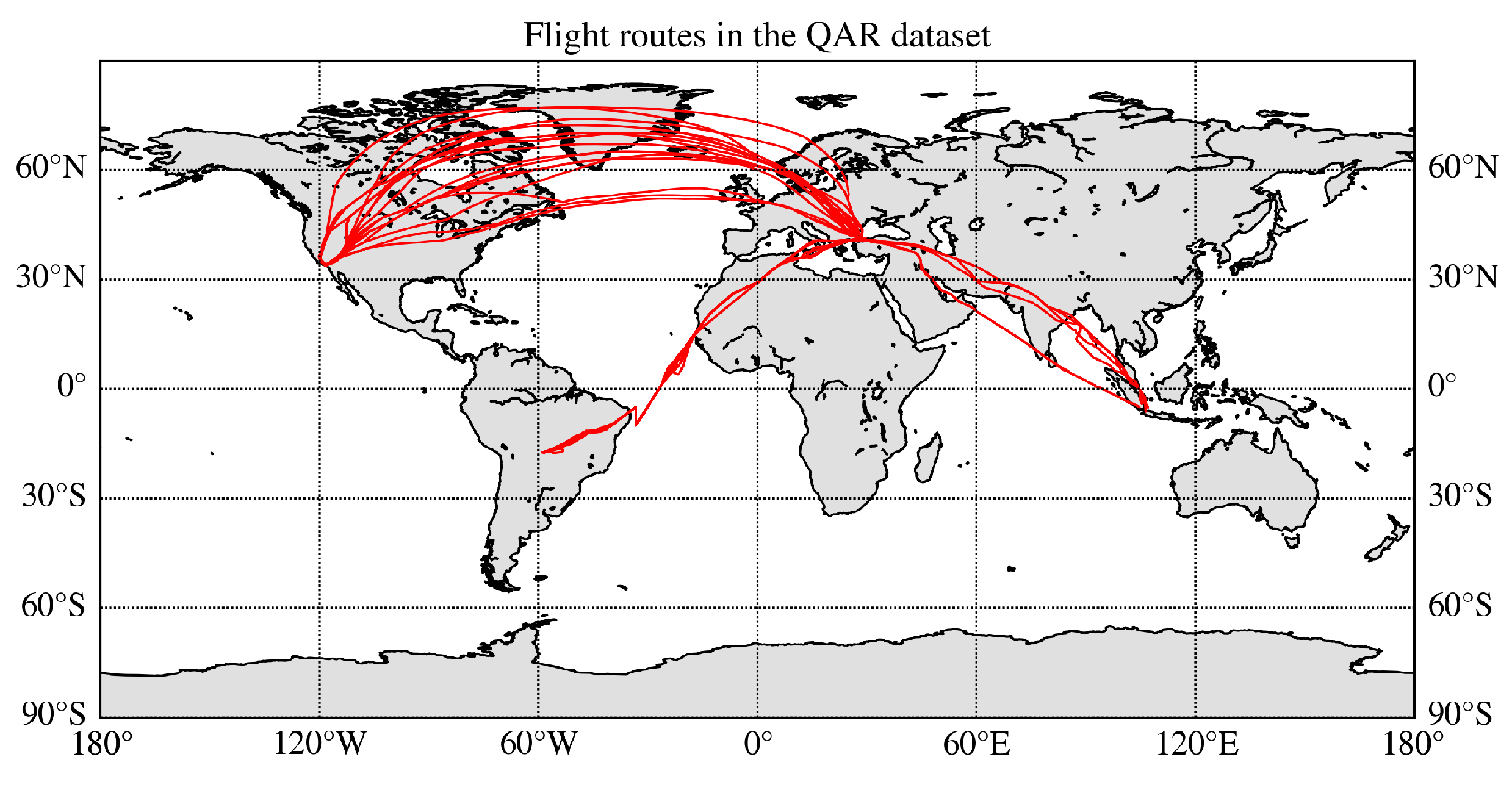
This work utilizes QAR data from a major European flag carrier airline for the design of deep learning neural network architectures. The dataset consists of myriads of features sampled at 1 Hz, which is the maximum recording frequency in flight data recording systems [52]. The dataset of interest for this study includes information about dynamic states of an aircraft (airspeed, altitude, position, vertical speed, and heading), body axis states (angle of attack, and longitudinal and lateral acceleration), performance states (throttle settings, fuel flow from engines, and mass), configuration states (high lift devices, landing gear, and speed brake) and environmental states (wind speed/direction, static and total temperature of air, and air pressure). Even though these states are the most critical variables used in this kind of research, a QAR device usually records more than 1000 features. Table 2 summarizes the variables selected from the QAR dataset used in this work. Because each individual aircraft differs at performance, we have used QAR dataset of a unique tail-number. Figure 8 depicts geospatial distribution of the flight routes in the training data.
During training, dataset of a particular tail-number aircraft is utilized. The data has 98 flights, 81 long haul and 17 short haul, with an amount of 2.6 M cruise points. Because the original QAR files are flight-based, they are comprised of the whole flight from take-off to landing, including taxi phases. Therefore, ground, climb and descent points should be separated to have solely cruise trajectories. We use the altitude gradient to check whether a point belongs to a level flight. Let X c r z be the cruise data:
X c r z = x [ i ] : | h ˙ [ i ] | 1 f t / s i = 1 N d
where x [ i ] = { δ [ i ] , θ [ i ] , M [ i ] , m a c [ i ] } , and h [ i ] is the corresponding altitude at ith element. As for the train-test split, we spared the first 90 flights for training, and the remaining 8 flights for testing. We selected standard scaling to scale the data. Let X t r n , X t s t and X ( . ) s c be the training, test, and scaled data, respectively. The scaled training data is:
X t r n s c = X t r n μ X t r n σ X t r n
The same parameters, namely the mean and standard deviation indicated in the equation above are applied to the test set as:
X t s t s c = X t s t μ X t r n σ X t r n
The complementary flight regime set R is independent from the data. Its elements are separate from the cruise data X c r z . There is no experiment in this paper to find the optimum number of elements of R . We selected two hundred distinct flight regimes consisting different values of altitude h, ISA temperature deviation Δ T , and aircraft mass m a c . Altitude and ISA deviation are sufficient to calculate pressure and temperature ratio through the following equations:
θ = T a m b 288.15 = 288.15 + Δ T I S A 0.0019812 h 288.15
δ = T a m b Δ T I S A 288.15 5.25588
For each combination of δ , θ , and m a c , we calculate the corresponding Mach number limits. The minimum Mach number is in which the aircraft is cruising at the maximum lift coefficient available, C L , m a x . This study utilizes BADA4 buffet limit model to calculate C L , m a x , and for now, it is the only point wherein this methodology requires an external performance model. We calculate the maximum Mach number given the maximum operable calibrated airspeed V C A S , m a x :
M m a x = 5 1 δ 1 + 0.2 V C A S , m a x 661.4786 2 3.5 1 + 1 1 3.5 1
For the aircraft in this study, the maximum operable calibrated airspeed is V C A S , m a x = 330 [kt] The minimum Mach speed is connected with altitude and aircraft mass. The flight regime sets in R are selected considering the aircraft limits, which are open-access information. The lower and upper limits of altitude, ISA deviation and aircraft mass are given in Table 3. The elements of R are triple combinations of altitude, ISA deviation, and aircraft mass within these boundaries. Then, BADA4 and Equation (49) calculate the Mach speed limits for each r n . Two examples are given below:
r 1 = 0.35 0.84 0.65 280 , 000 0.35 0.84 0.653 280 , 000 0.35 0.84 0.657 280 , 000 0.35 0.84 0.837 280 , 000 0.35 0.84 0.84 280 , 000 r 2 = 0.22 0.76 0.76 245 , 000 0.22 0.76 0.764 245 , 000 0.22 0.76 0.769 245 , 000 0.22 0.76 0.883 245 , 000 0.22 0.76 0.89 245 , 000
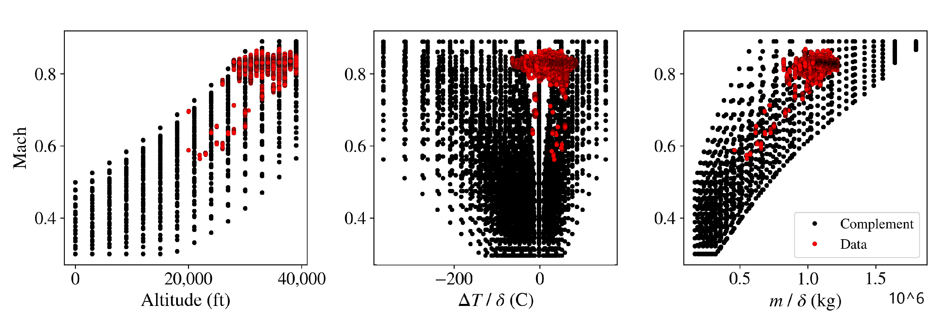
Figure 9 illustrates the envelope covered in the data, and the flight regimes included. On the left, there is altitude versus Mach, and it shows that most of the flights are above 30,000 feet. The rest is highly sparse and there is almost none at altitudes below 20,000 feet. The middle sub-figure represents Mach distribution over ISA deviation. To generalize it, we divided ISA deviation by pressure ratio. Otherwise, there is no inter-dependency between ISA deviation and Mach. Under the limits, an aircraft can fly at all Mach speeds with all ISA deviation values. In the data, observed ISA deviations are between 25 C and 20 C. We expanded this regime to have more temperature ratio values to provide to the algorithm. Lastly, the plot on the right depicts Mach distribution over aircraft mass. Likewise, aircraft mass is divided by pressure ratio for generalization. As an aircraft gets lighter after burning fuel, it either increase its speed or altitude for flight efficiency. In real-world operations, this appears as step climbs after cruising some distances. Therefore, the Mach variance in the data is low, because the aircraft usually maintains the speed, but increase the altitude. This has another effect as well, which is the rarity of observing high aircraft masses at higher altitudes. Whenever an aircraft of this study does its third or fourth step climb, it is ordinarily lighter than 260 tons. Therefore, many of the feasible altitude—mass pairs are not available in data.
The tolerance value F t o l is selected to be 4000 [kg/h]. This magnitude is heuristic, and based on simulation results using BADA4. Hyper-parameters are λ e = 1.0 , λ s = 10 6 , λ P H Y , 1 = 0.8 , λ P H Y , 2 = 0.2 , and λ P H Y , 3 = 0.8 . Note that the elements of R are also scaled through Equation (45). For more efficient stochastic gradient descent, the training data X t r n s c is divided into mini-batches with a size of 1024. He initialization [53] is selected to assign the initial states of W [ l ] and b [ l ] . The learning process utilizes the AdaBound optimization algorithm [54] to update weight matrices W and bias vectors b at each step k:
ξ k + 1 = ξ k + A d a B o u n d J x t r n [ k ] , s c , R ζ , α
We tuned the learning rate α by checking the status of the loss function. If the loss function is not improved 10 times consecutively, the learning rate α is reduced by 90%. Its initial value is chosen as 0.001. The models are trained for 1000 epochs. Five hidden layers are used and the neuron numbers are { 1024 , 512 , 256 , 128 , 32 } . The deep neural network models are implemented and trained with PyTorch framework [55].
We compare the model with other linear and non-linear function approximation algorithms. These are linear regression L R , support vector regression S V R , neural network with one hidden layer N N , and deep neural network D N N without including physics loss. Additionally, fuel consumption calculations from BADA4 is provided. The model denoted by B A D A 4 * is the baseline BADA4 fuel consumption calibrated through linear regression. Two different error metrics, namely the mean absolute error and the mean absolute percentage error are presented in Table 4. The results indicate that deep neural networks yield the lowest prediction errors. This implies the necessity of universal function approximators for capturing fuel consumption dynamics better.
M A E = 1 N d i N d y ^ d [ i ] y d [ i ]
M A P E = 100 × 1 N d i N d y ^ d [ i ] y d [ i ] y d [ i ]
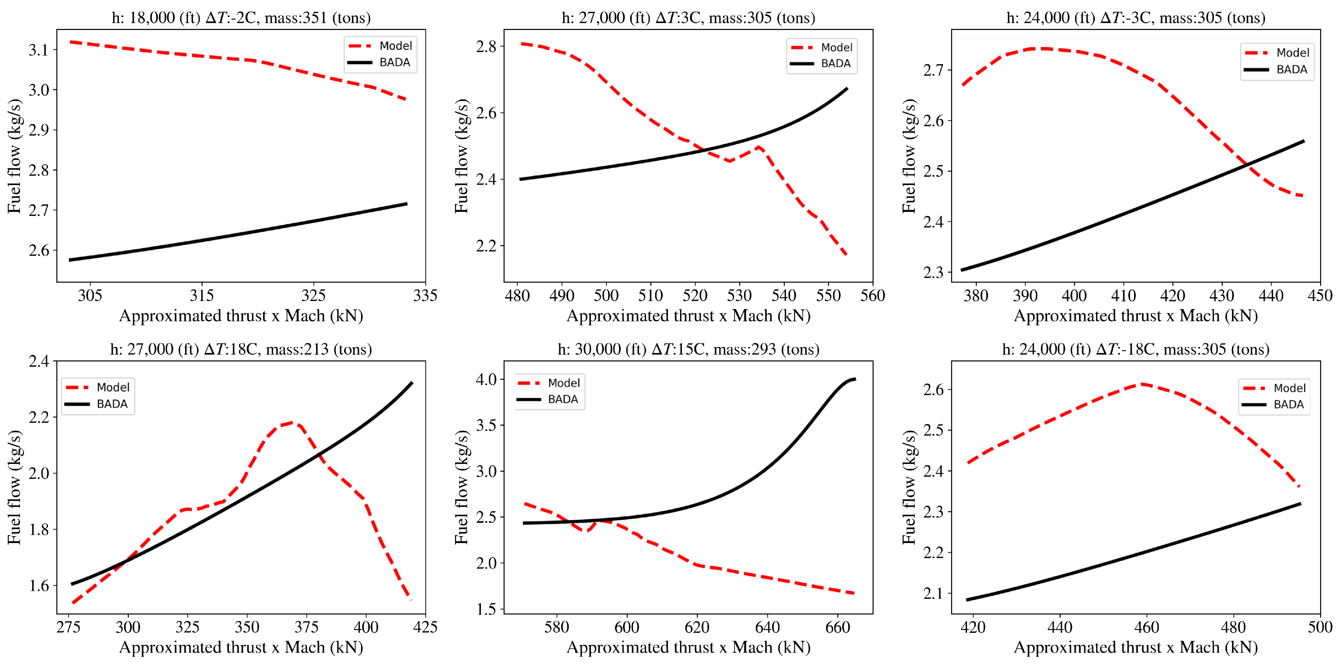
Fuel consumption prediction errors of the generic deep neural network and our physics informed network are shown to be very close on the test set. The main discrepancy between these designs lies in their respective physical consistencies. As illustrated in Figure 7, we expect any physically consistent model to produce an increasing fuel consumption profile with an increasing thrust times Mach input, given an altitude, a ISA deviation, and a reference mass. Figure 10 demonstrates fuel consumption predicted by the generic deep neural network model for six different cases of flight conditions. Even though this model accurately captures the fuel consumption trajectories on the test set, it performs poorly in terms of physical consistency. All fuel consumption profiles in these six regimes have decaying parts, with growing thrust times Mach. Moreover, the behavior is not homogeneous, i.e., the model does not always yield monotonic decreasing curves.
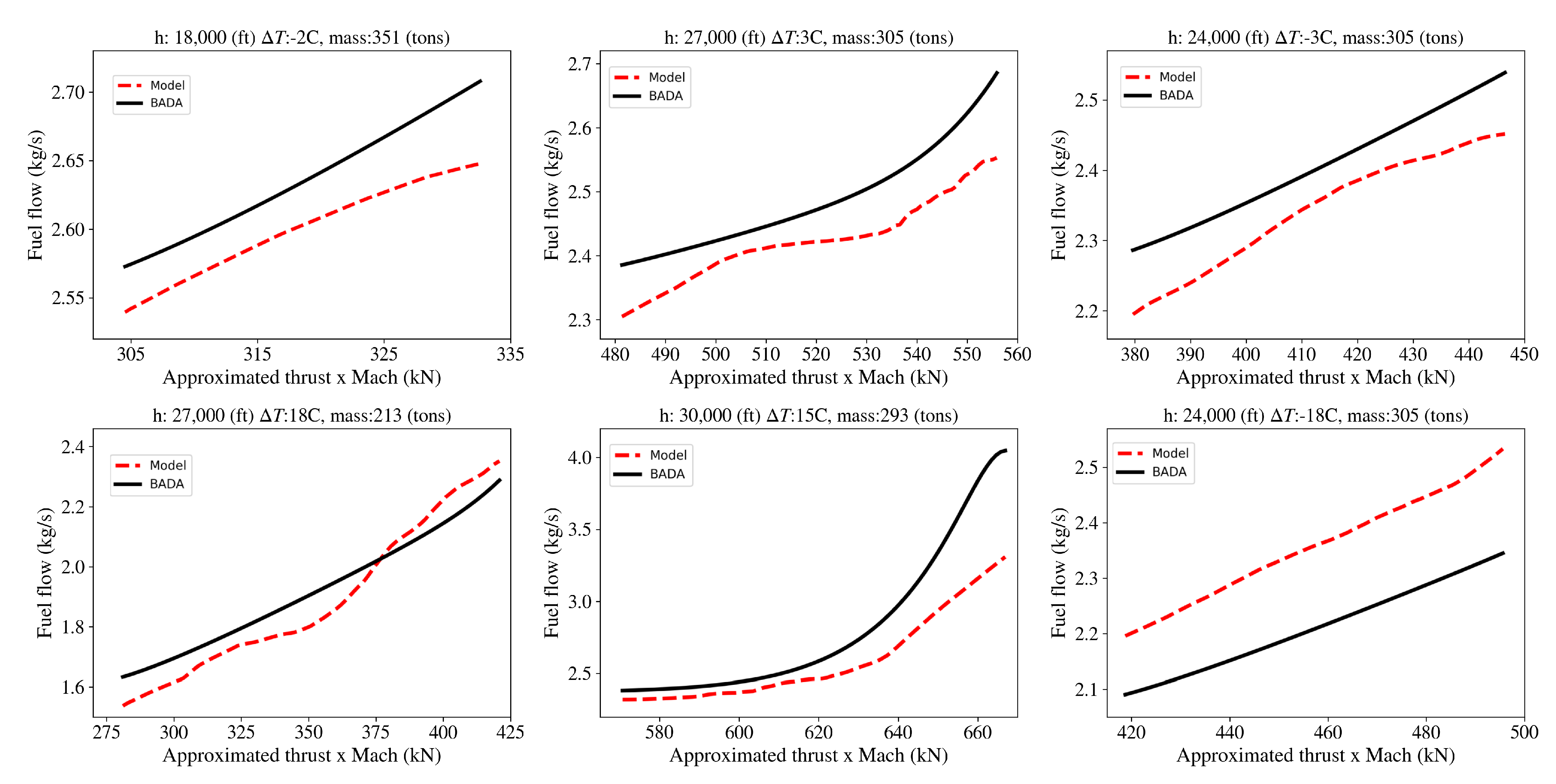
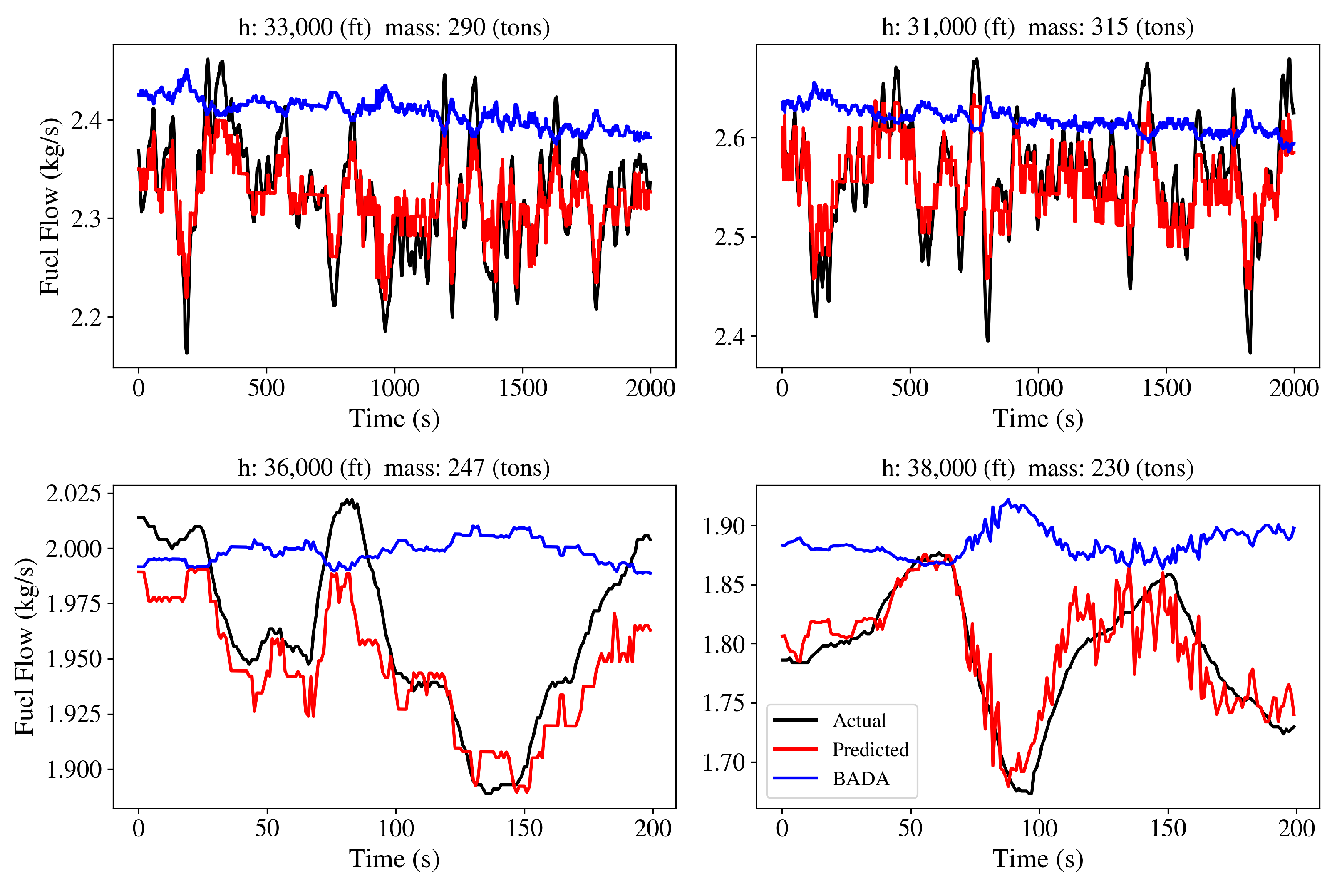
On the other hand, our proposed model, which includes physical loss functions, complies with the physical intuition. Figure 11 reveals that fuel consumption trajectories predicted with the proposed neural network model grow as thrust times Mach values increase. They are not always entirely linear, but do not violate the physics. Additionally, in many cases fuel consumption curves predicted with the trained model is under the ones computed by BADA4. This shows that model-based approaches tend to overestimate fuel consumption for this tail-number aircraft. There are some exceptions, like the example in right-bottom plot in Figure 11. However, we do not have labeled data for this flight regime to justify whether our prediction is very close to the actual. Still, as can be seen in Figure 12, the proposed model adequately predicts the fuel consumption profiles of the test set. Compared to our model, BADA4 overestimates fuel consumption in the test set. Furthermore, our model is able to capture the unknown patterns that BADA4 does not cover. Zoomed regression plots show that the model is able to predict short-period fluctuations. These are due to autopilot modules that control the angle of attack and throttle to maintain level flight. Because NNs are universal function approximators, they can establish such mappings that curve fitting algorithms fail.
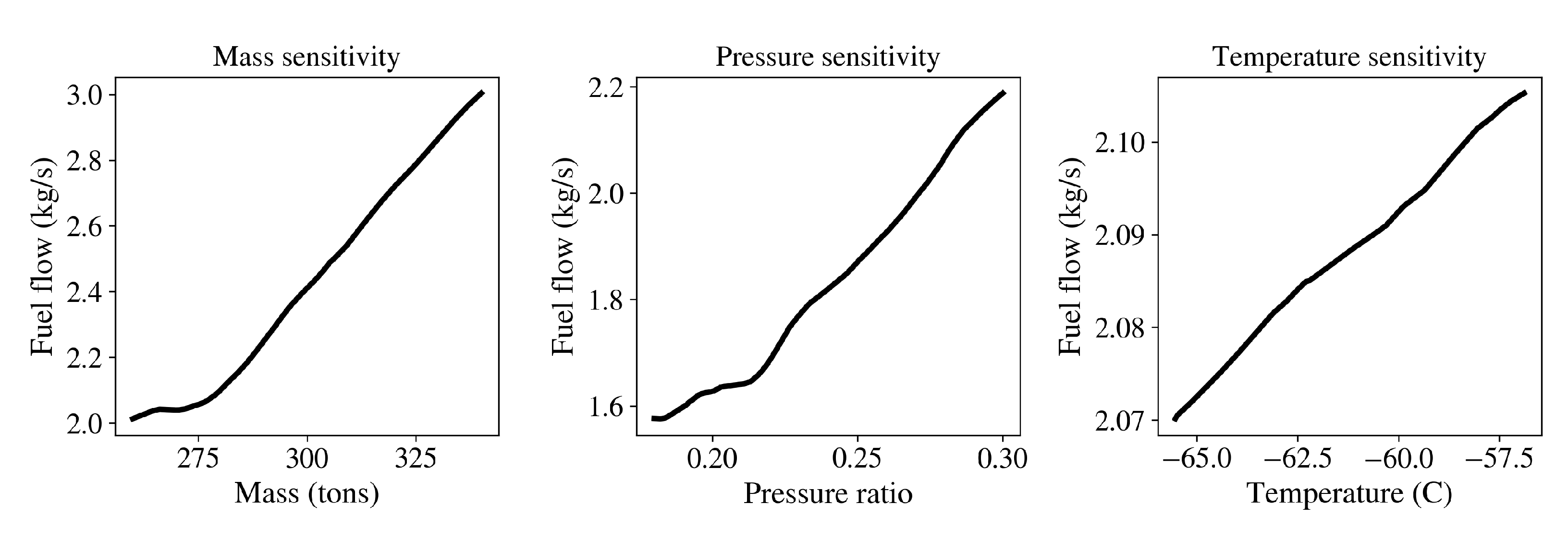
Additionally, we show the model’s sensitivity to the other parameters; namely the pressure ratio, temperature ratio, and mass in Figure 13. Because these variables have enough variance in the data, the sensitivity lines are meaningful without including additional loss terms. Among these parameters, temperature is output of a forecast in flight planning. It usually appears at high accuracy, but it is still possible to correct weather uncertainty using data-driven techniques, as well [8]. In conclusion, appending additional loss terms to the empirical error does not diminish the supervised learning performance. Properly selected loss functions even enable the deep neural network to capture further dynamics and flight regimes that data sets do not actually cover.

6. Conclusions

In this work, we have considered the fuel consumption estimation problem of an aircraft using QAR flight data for flight trajectory planning and estimation. Specifically, we have focused on the cruise segment of flight, which is the critical segment for fuel efficient flight planning in long-haul flights. Our results show that the standard machine learning algorithms as developed within the literature, although providing high precision input-output relationships within the given flight envelope of the data, fail to capture the fundamental physical principles of fuel consumption once utilized over the whole flight envelope. Thus the applicability of such neural network models for flight planning over the whole flight envelope is questionable. As to solve this critical issue, we have designed a novel physics guided deep learning method to capture not only the nonlinear relationships between the key variables within the flight data, but also the physics of flight and fuel consumption as denoted by model-based approaches. Our proposed method relies on the introduction of learning loss functions which embed the underlying physical principles and aircraft constraints. The resulting neural network structures are shown to produce high precision fuel consumption models within the flown flight regimes and physically consistent solutions across the whole flight envelope. It is important to note that without the availability of data in unforeseen flight regimes, it is impossible to fully quantify the precision of the model over the whole flight envelope. However, our results show that our deep learning model produces fuel consumption predictions which are inline with the BADA4 calculations in unseen flight regimes. Thus, including key physical principles in the training/learning phase of purely data-driven models increases accuracy, explainability and generalization capability of the developed models. To the best of our knowledge, this is the first work that successfully designs and demonstrates a physics-guided deep learning framework in fuel consumption modeling for an aircraft.
The most challenging part of this study is selecting the loss terms’ weights. We envision seeking methods such as Bayesian optimization to standardize this procedure. Additionally, even though our model yields physically coherent outputs, accuracy on unlabeled flight regimes is still an open issue. One possible approach could be providing initial guesses using existing performance models, but it would diminish the independence. In conclusion, our current work focuses on the effects of using particular deep learning architectures on the fuel flow estimation accuracy. Specifically, we investigate the neural architecture search algorithms’ performance for this problem. As such, novel deep learning models considering the input feature interactions more effectively or further considering autoencoder-based deep embedding models are envisioned to improve fuel consumption estimation success.

Author Contributions

Conceptualization, M.U. and M.U.D.; Funding acquisition, G.I.; Methodology, M.U. and M.U.D.; Project administration, G.I.; Software, M.U.; Supervision, M.U.D. and G.I.; Visualization, M.U.; Writing—original draft, M.U.; Writing—review and editing, M.U., M.U.D. and G.I. All authors have read and agreed to the published version of the manuscript.

Funding

This work is supported in part by Boeing Grants GT-187-1 and GT-057-1.

Institutional Review Board Statement

Not applicable.

Informed Consent Statement

Not applicable.

Acknowledgments

We would like to thank Boeing for providing technical guidance on aircraft performance modeling and fuel consumption models.

Conflicts of Interest

The authors declare no conflict of interest.

Abbreviations

The following abbreviations are used in this manuscript:
QARQuick Access Recorder
MLPMulti-layer Perceptron
OEMOriginal Equipment Manufacturer
BADABase of Aircraft Data
MLMachine Learning
DLDeep Learning
NNNeural Networks
DNNDeep Neural Networks
MAEMean Absolute Error
MAPEMean Absolute Percentage Error

References

  1. Gallo, E.; Lopez-Leones, J.; Vilaplana, M.A.; Navarro, F.A.; Nuic, A. Trajectory computation infrastructure based on BADA aircraft performance model. In Proceedings of the 2007 IEEE/AIAA 26th Digital Avionics Systems Conference, Dallas, TX, USA, 21–25 October 2007; pp. 1.C.4-1–1.C.4-13. [Google Scholar]
  2. Jensen, L.; Hansman, R.J.; Venuti, J.C.; Reynolds, T. Commercial airline speed optimization strategies for reduced cruise fuel consumption. In Proceedings of the 2013 Aviation Technology, Integration, and Operations Conference, Los Angeles, CA, USA, 12–14 August 2013; p. 4289. [Google Scholar]
  3. Malaek, S.; Alaeddini, A.; Gerren, D. Optimal maneuvers for aircraft conflict resolution based on efficient genetic webs. IEEE Trans. Aerosp. Electron. Syst. 2011, 47, 2457–2472. [Google Scholar] [CrossRef]
  4. Rodrigues, L. A unified optimal control approach for maximum endurance and maximum range. IEEE Trans. Aerosp. Electron. Syst. 2017, 54, 385–391. [Google Scholar] [CrossRef]
  5. Brown, A.; Anderson, D. Trajectory optimization for high-altitude long endurance UAV maritime radar surveillance. IEEE Trans. Aerosp. Electron. Syst. 2019, 56, 2406–2421. [Google Scholar] [CrossRef] [Green Version]
  6. Wasiuk, D.; Lowenberg, M.; Shallcross, D. An aircraft performance model implementation for the estimation of global and regional commercial aviation fuel burn and emissions. Transp. Res. Part D Transp. Environ. 2015, 35, 142–159. [Google Scholar] [CrossRef] [Green Version]
  7. Uzun, M.; Demirezen, M.U.; Koyuncu, E.; Inalhan, G. Design of a Hybrid Digital-Twin Flight Performance Model through Machine Learning. In Proceedings of the 2019 IEEE Aerospace Conference, Big Sky, MT, USA, 2–9 March 2019; pp. 1–14. [Google Scholar]
  8. Uzun, M.; Demirezen, M.U.; Koyuncu, E.; Inalhan, G.; Lopez, J.; Vilaplana, M. Deep Learning Techniques for Improving Estimations of Key Parameters for Efficient Flight Planning. In Proceedings of the 2019 IEEE/AIAA 38th Digital Avionics Systems Conference (DASC), San Diego, CA, USA, 8–12 September 2019; pp. 1–8. [Google Scholar]
  9. Sun, J.; Hoekstra, J.M.; Ellerbroek, J. OpenAP: An Open-Source Aircraft Performance Model for Air Transportation Studies and Simulations. Aerospace 2020, 7, 104. [Google Scholar] [CrossRef]
  10. Baumann, S.; Klingauf, U. Modeling of aircraft fuel consumption using machine learning algorithms. CEAS Aeronaut. J. 2020, 11, 277–287. [Google Scholar] [CrossRef]
  11. Swischuk, R.C.; Allaire, D.L. A Machine Learning Approach to Aircraft Sensor Error Detection and Correction. J. Comput. Inf. Sci. Eng. 2019, 19, 041009. [Google Scholar] [CrossRef]
  12. Behjat, A.; Zeng, C.; Rai, R.; Matei, I.; Doermann, D.; Chowdhury, S. A physics-aware learning architecture with input transfer networks for predictive modeling. Appl. Soft Comput. 2020, 96, 106665. [Google Scholar] [CrossRef]
  13. Vabalas, A.; Gowen, E.; Poliakoff, E.; Casson, A.J. Machine learning algorithm validation with a limited sample size. PLoS ONE 2019, 14, e0224365. [Google Scholar] [CrossRef]
  14. Rad, K.R.; Zhou, W.; Maleki, A. Error bounds in estimating the out-of-sample prediction error using leave-one-out cross validation in high-dimensions. In Proceedings of the Twenty Third International Conference on Artificial Intelligence and Statistics; Chiappa, S., Calandra, R., Eds.; Proceedings of Machine Learning Research (PMLR), 2020; Volume 108, pp. 4067–4077. Available online: https://arxiv.org/pdf/2003.01770v1.pdf (accessed on 2 November 2020).
  15. Wu, Z.; Li, X.; Du, J. Fuel Consumption Model of Aircraft in Descent Stage Based on DBN. IOP Conf. Ser. Mater. Sci. Eng. 2019, 569, 032005. [Google Scholar] [CrossRef]
  16. Chati, Y.S.; Balakrishnan, H. Data-Driven Modeling of Aircraft Engine Fuel Burn in Climb Out and Approach. Transp. Res. Rec. 2018, 2672, 1–11. [Google Scholar] [CrossRef]
  17. Muralidhar, N.; Bu, J.; Cao, Z.; He, L.; Ramakrishnan, N.; Tafti, D.; Karpatne, A. Physics-Guided Deep Learning for Drag Force Prediction in Dense Fluid-Particulate Systems. Big Data 2020, 8, 431–449. [Google Scholar] [CrossRef] [PubMed]
  18. Muralidhar, N.; Islam, M.R.; Marwah, M.; Karpatne, A.; Ramakrishnan, N. Incorporating prior domain knowledge into deep neural networks. In Proceedings of the 2018 IEEE International Conference on Big Data (Big Data), Seattle, WA, USA, 10–13 December 2018; pp. 36–45. [Google Scholar]
  19. Misyris, G.S.; Venzke, A.; Chatzivasileiadis, S. Physics-informed neural networks for power systems. In Proceedings of the 2020 IEEE Power & Energy Society General Meeting (PESGM), Montreal, QC, Canada, 2–6 August 2020; pp. 1–5. [Google Scholar]
  20. Yucesan, Y.A.; Viana, F.A. A physics-informed neural network for wind turbine main bearing fatigue. Int. J. Progn. Health Manag. 2020, 11, 17. [Google Scholar]
  21. Read, J.S.; Jia, X.; Willard, J.; Appling, A.P.; Zwart, J.A.; Oliver, S.K.; Karpatne, A.; Hansen, G.J.; Hanson, P.C.; Watkins, W.; et al. Process-guided deep learning predictions of lake water temperature. Water Resour. Res. 2019, 55, 9173–9190. [Google Scholar] [CrossRef] [Green Version]
  22. Rai, R.; Sahu, C.K. Driven by Data or Derived Through Physics? A Review of Hybrid Physics Guided Machine Learning Techniques With Cyber-Physical System (CPS) Focus. IEEE Access 2020, 8, 71050–71073. [Google Scholar] [CrossRef]
  23. Shukla, K.; Di Leoni, P.C.; Blackshire, J.; Sparkman, D.; Karniadakis, G.E. Physics-Informed Neural Network for Ultrasound Nondestructive Quantification of Surface Breaking Cracks. J. Nondestruct. Eval. 2020, 39, 61. [Google Scholar] [CrossRef]
  24. Zamzam, A.S.; Sidiropoulos, N.D. Physics-aware neural networks for distribution system state estimation. IEEE Trans. Power Syst. 2020, 35, 4347–4356. [Google Scholar] [CrossRef] [Green Version]
  25. Todd, J.C. Flight Data Recorder System. U.S. Patent 6,397,128, 28 May 2002. [Google Scholar]
  26. Wang, L.; Wu, C.; Sun, R. An analysis of flight Quick Access Recorder (QAR) data and its applications in preventing landing incidents. Reliab. Eng. Syst. Saf. 2014, 127, 86–96. [Google Scholar] [CrossRef]
  27. Sembiring, J.; Drees, L.; Holzapfel, F. Extracting unmeasured parameters based on quick access recorder data using parameter-estimation method. In Proceedings of the AIAA Atmospheric Flight Mechanics (AFM) Conference, Boston, MA, USA, 19–22 August 2013; p. 4848. [Google Scholar]
  28. Luo, H.; Zhong, S. Gas turbine engine gas path anomaly detection using deep learning with Gaussian distribution. In Proceedings of the 2017 Prognostics and System Health Management Conference (PHM-Harbin), Harbin, China, 9–12 July 2017; pp. 1–6. [Google Scholar]
  29. Chati, Y.S.; Balakrishnan, H. Aircraft engine performance study using flight data recorder archives. In Proceedings of the 2013 Aviation Technology, Integration, and Operations Conference, Los Angeles, CA, USA, 12–14 August 2013; p. 4414. [Google Scholar]
  30. Chati, Y.S.; Balakrishnan, H. Statistical modeling of aircraft engine fuel flow rate. In Proceedings of the 30th Congress of the International Council of the Aeronautical Science, Daejeon, Korea, 25–30 September 2016. [Google Scholar]
  31. Chati, Y.S.; Balakrishnan, H. A Gaussian process regression approach to model aircraft engine fuel flow rate. In Proceedings of the 2017 ACM/IEEE 8th International Conference on Cyber-Physical Systems (ICCPS), Pittsburgh, PA, USA, 18–21 April 2017; pp. 131–140. [Google Scholar]
  32. Baklacioglu, T. Modeling the fuel flow-rate of transport aircraft during flight phases using genetic algorithm-optimized neural networks. Aerosp. Sci. Technol. 2016, 49, 52–62. [Google Scholar] [CrossRef]
  33. Huang, C.; Xu, Y.; Johnson, M.E. Statistical modeling of the fuel flow rate of GA piston engine aircraft using flight operational data. Transp. Res. Part D Transp. Environ. 2017, 53, 50–62. [Google Scholar] [CrossRef]
  34. Khadilkar, H.; Balakrishnan, H. Estimation of aircraft taxi fuel burn using flight data recorder archives. Transp. Res. Part D Transp. Environ. 2012, 17, 532–537. [Google Scholar] [CrossRef]
  35. Hornik, K.; Stinchcombe, M.; White, H. Multilayer feedforward networks are universal approximators. Neural Netw. 1989, 2, 359–366. [Google Scholar] [CrossRef]
  36. Roberson, B. Fuel Conservation Strategies: Cost index explained. Boeing Aero Q. 2007, 2, 26–28. [Google Scholar]
  37. Abu-Mostafa, Y.S. Learning from hints in neural networks. J. Complex. 1990, 6, 192–198. [Google Scholar] [CrossRef] [Green Version]
  38. Liu, D.C.; Nocedal, J. On the limited memory BFGS method for large scale optimization. Math. Program. 1989, 45, 503–528. [Google Scholar] [CrossRef] [Green Version]
  39. Rahmani, F.; Lawson, K.; Ouyang, W.; Appling, A.; Oliver, S.; Shen, C. Exploring the exceptional performance of a deep learning stream temperature model and the value of streamflow data. Environ. Res. Lett. 2020, 16, 024025. [Google Scholar]
  40. Ramadhan, A.; Marshall, J.; Souza, A.; Wagner, G.L.; Ponnapati, M.; Rackauckas, C. Capturing missing physics in climate model parameterizations using neural differential equations. arXiv 2020, arXiv:2010.12559. [Google Scholar]
  41. Winkler, D.A.; Le, T.C. Performance of deep and shallow neural networks, the universal approximation theorem, activity cliffs, and QSAR. Mol. Inform. 2017, 36, 1600118. [Google Scholar] [CrossRef] [Green Version]
  42. Chen, T.; Chen, H. Universal approximation to nonlinear operators by neural networks with arbitrary activation functions and its application to dynamical systems. IEEE Trans. Neural Netw. 1995, 6, 911–917. [Google Scholar] [CrossRef] [Green Version]
  43. Rumelhart, D.E.; Hinton, G.E.; Williams, R.J. Learning representations by back-propagating errors. Nature 1986, 323, 533–536. [Google Scholar] [CrossRef]
  44. Srivastava, N.; Hinton, G.; Krizhevsky, A.; Sutskever, I.; Salakhutdinov, R. Dropout: A Simple Way to Prevent Neural Networks from Overfitting. J. Mach. Learn. Res. 2014, 15, 1929–1958. [Google Scholar]
  45. Nuic, A.; Poinsot, C.; Iagaru, M.G.; Gallo, E.; Navarro, F.A.; Querejeta, C. Advanced aircraft performance modeling for ATM: Enhancements to the BADA model. In Proceedings of the 24th Digital Avionics System Conference, AIAA/IEEE, Washington, DC, USA, 30 October–3 November 2005; pp. 1–14. [Google Scholar]
  46. Airbus Customer Services. Getting to Grips with Aircraft Performance; Technical Report; Airbus Customer Services: Blagnac, France, 2002. [Google Scholar]
  47. Anderson, D. Cruise Performance Monitoring. Boeing Aero Magazine. 2006, pp. 5–11. Available online: http://www.boeing.com/commercial/aeromagazine/articles/qtr_4_06/AERO_Q406_article2.pdf (accessed on 2 November 2020).
  48. Mouillet, V.; Nuić, A.; Casado, E.; Leonés, J.L. Evaluation of the Applicability of a Modern Aircraft Performance Model to Trajectory Optimization. In Proceedings of the 2018 IEEE/AIAA 37th Digital Avionics Systems Conference (DASC), London, UK, 23–27 September 2018; pp. 1–9. [Google Scholar]
  49. Yechout, T.R. Introduction to Aircraft Flight Mechanics; Aiaa: Blacksburg, VA, USA, 2003; pp. 68–75. [Google Scholar]
  50. Center, E.E. User Manual for the Base of Aircraft Data (BADA) Revison 3.11; Eurocontrol: Brussels, Belgium, 2013. [Google Scholar]
  51. Blake, W. Jet Transport Performance Methods; Boeing Commercial Airplanes: Seattle, WA, USA, 2009; Volume 6-1420. [Google Scholar]
  52. Sudolsky, M. ARINC 573/717, 767 and 647A: The Logical Choice for Maintenance Recording And IVHM Interface Control or Frame Updates. In Proceedings of the Prognostics and Health Management Society, San Diego, CA, USA, 27 September–1 October 2009. [Google Scholar]
  53. He, K.; Zhang, X.; Ren, S.; Sun, J. Delving deep into rectifiers: Surpassing human-level performance on imagenet classification. In Proceedings of the IEEE International Conference on Computer Vision, Santiago, Chile, 7–13 December 2015; pp. 1026–1034. [Google Scholar]
  54. Luo, L.; Xiong, Y.; Liu, Y. Adaptive Gradient Methods with Dynamic Bound of Learning Rate. arXiv 2019, arXiv:1902.09843.8024. [Google Scholar]
  55. Paszke, A.; Gross, S.; Massa, F.; Lerer, A.; Bradbury, J.; Chanan, G.; Killeen, T.; Lin, Z.; Gimelshein, N.; Antiga, L.; et al. Pytorch: An imperative style, high-performance deep learning library. In Proceedings of the Advances in Neural Information Processing Systems 32, Vancouver, BA, Canada, 8–14 December 2019; pp. 8024–8035. [Google Scholar]
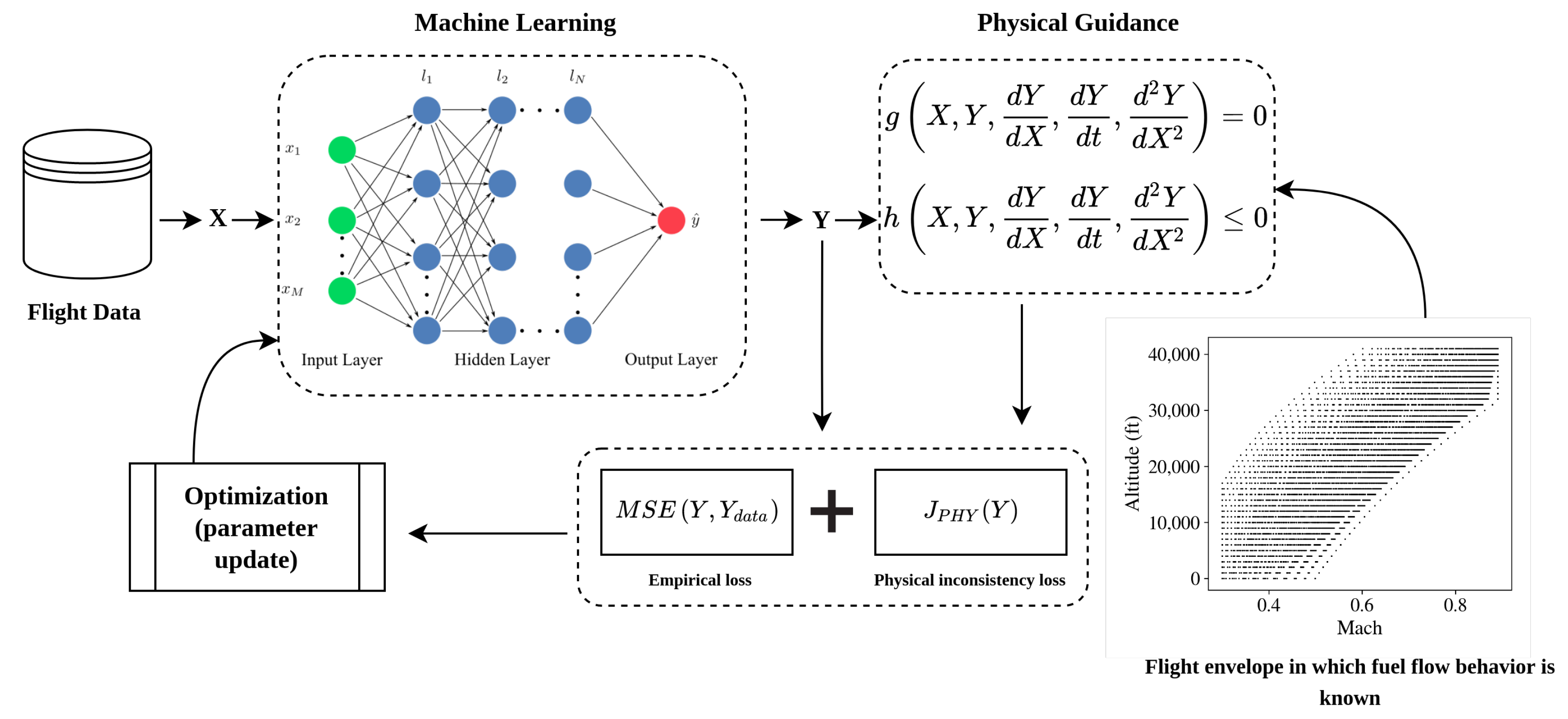
Figure 1. The hybrid system consisting of neural networks, and physics-guidance.
Aerospace 08 00044 g001
Figure 2. Generic architecture of a Multi-Layer Perceptron.
Aerospace 08 00044 g002
Figure 3. Thrust required with increasing Mach number and mass.
Aerospace 08 00044 g003
Figure 4. Mach number vs. fuel consumption for selected atmospheric conditions, and gross weight.
Aerospace 08 00044 g004
Figure 5. Distributions of parameters from QAR dataset.
Aerospace 08 00044 g005
Figure 6. The effect of gross weight on throttle setting and fuel consumption.
Aerospace 08 00044 g006
Figure 7. Thrust times Mach versus fuel consumption for various flight regimes.
Aerospace 08 00044 g007
Figure 8. Lateral profiles of the flights in the dataset.
Aerospace 08 00044 g008
Figure 9. Full flight envelope compared to the regimes represented in the data.
Aerospace 08 00044 g009
Figure 10. Mach sensitivity of the model without including physics.
Aerospace 08 00044 g010
Figure 11. Mach sensitivity of the model with including physics.
Aerospace 08 00044 g011
Figure 12. Fuel consumption prediction with the trained physics-guided NN model.
Aerospace 08 00044 g012
Figure 13. Model sensitivity to pressure ratio, temperature ratio, and mass.
Aerospace 08 00044 g013
Table 1. Summary of flight and atmospheric parameters that affect fuel consumption.
ApproachParameters That Affect Fuel Consumption
Model-basedPressure ratio δ , temperature ratio θ , throttle δ T , Mach number M
Data-drivenPressure ratio δ , temperature ratio θ , throttle δ T , mass m a c , true airspeed V
Table 2. Summary of parameters directly used from QAR dataset.
hBarometric altitude [ft]
T c Static air temperature [C]
V C A S Calibrated airspeed [kt]
MMach speed
m a c Aircraft mass [kg]
F e n g Fuel flow from engines [lb/hr]
T r 1 , 2 Throttle positions of engines 1 and 2
V w i n d Wind speed [kt]
χ W i n d Wind direction [deg]
χ a c True heading [deg]
δ f l a p Flap deflection [deg]
δ l g Landing gear status { 0 , 1 }
δ s b Speed break deflection [deg]
F a p u APU fuel consumption [lb/hr]
Table 3. Operational altitude, ISA deviation, and aircraft mass limits.
ParameterMinMax
Altitude h (ft)041,000
ISA deviation Δ T (C)−7750
Mass m a c (kg)167,000353,000
Table 4. Comparison of prediction results on the test set.
CriteriaBADA4 BADA 4 * SVRLRNNDNNProposed
MAE [kg/h]291215195201172127133
MAPE %3.7122.6322.6772.6951.8971.5211.568
Publisher’s Note: MDPI stays neutral with regard to jurisdictional claims in published maps and institutional affiliations.