Analysis of Aircraft Operation System Regarding Readiness—Case Study

Abstract

The aim of the study was to develop a model of the readiness and reliability of an aircraft to perform an air task. The applied research method uses quantitative statistical methods and Markov processes in order to create a mathematical algorithm to exploit a selected aircraft type. The paper presents a case study of the TS-11 “Iskra” aircraft. The results show that even if the probability of being on stand-by is low, the tasks can be completed by operating the entire fleet properly.

1. Introduction

1.1. Operation Process

Aircraft maintenance is a complex process aimed at ensuring safe performance of aviation tasks. In aviation, we can distinguish between exploitation strategy according to service life or technical condition. Nowadays, in order to ensure maximum efficiency of task execution, a mixed method is used with increasing frequently [1].

Maintenance involves carrying out work on the aircraft according to a strictly defined schedule. The maintenance program must provide information about which aircraft components should be replaced or renewed after a specified flight time or number of completed tasks. The disadvantage of the aforementioned maintenance program, according to the survey regarding the aircraft’s readiness to perform the operations in the context of safety and effectiveness, concerns the possibility of replacing a part which meets all the standards, thereby increasing the costs for the maintenance user [2,3].

Condition-based equipment operation involves replacing or repairing components only when they show signs of wear. This method seems to be more economical due to more rational parts management. It should be noted, however, that non-destructive testing, necessary to assess the suitability of a part for further use, requires a lot of experience and knowledge from the person carrying out the testing and specialized equipment. This strategy proves to be cost-effective with a large fleet of aircraft where valuable testing equipment can work on many aircraft [4].

Due to the introduction of the AJT programme in the Air Force, it was decided that starting from 2016 the TS-11 aircraft will be serviced using the outsourcing method. The above decision resulted from the increase in the number of serviced aircraft while maintaining a constant number of ground staff. It was decided to transfer the periodic and current maintenance and repairs to an external entity (WZL No. 1 in Dęblin), while maintaining the maintenance system in the stationing unit to the extent necessary to secure the flights. Experience and extensive technical facilities allow Military Aviation Works to perform all work specified in the contracts without affecting the safety of flight tasks.

1.2. Reliability of Aircraft

In the available literature, it is possible to find a number of papers which demonstrate the problem of the impact of the external environment, ageing and wear processes on the technical system functioning [5,6]. Due to technical advancement and a high degree of integration of the devices used on board aircraft, the development of optimal operation models is a complex task. The methods for evaluating the reliability and durability of aviation equipment based on a change in diagnostic parameters are extremely useful within this area [7].

The impact of the materials used in the construction of an aircraft and the implemented technologies that affect its reliability and correct operation has been highlighted. The dominant approaches to aircraft reliability modelling can be divided into two main trends related to the analytical methods [8,9] as well as probabilistic approaches [10,11]. The method by which reliability is determined often depends on whether the failure of a component or of a complex structure is being studied. The treatment of the issue also depends on the failing history of the technical object in question. It is often the case that the reliability assessor does not have full documentation and knowledge of the testing and reliability of the components from which the aircraft is built, and does not take into account its design as well as the physical phenomena and operating conditions that may affect the faster ageing of the component [12]. With the development of diagnostic techniques, the system element approach is becoming more common. However, it should be remembered that often, e.g., in the case of flight training planning or tasks to be performed, it is more important for the investigator to take a binary approach as to whether the aircraft will be operational or not. In such a case, a monolithic approach is used. Mathematical modelling such as Markov [9] and semi-Markov [13] processes can be used to determine this relationship.

This paper includes a probabilistic method which it is recommended is used in order to determine the probability of an aircraft’s readiness to perform its missions during its life. The technical condition of some aviation equipment can be assessed with the use of diagnostic parameters. This assessment requires knowledge of limit (acceptable) values, for which it is considered that the device or assembly is in a state of usability.

2. Case Study

2.1. TS-11 “Iskra”

The TS-11 “Iskra” aircraft (Figure 1) has been the basic equipment in the process of training pilots of the Polish Air Force for many years. The origins of the aircraft can be traced back to 1957, when the design bureau under the leadership of docent engineer Tadeusz Sołtyk was commissioned to develop a preliminary design of the aircraft, including its tactical and technical requirements.

After the required ground tests had been carried out, the airplane was flown by the pilot Andrzej Abłamowicz in 1961, and two years later it was introduced into the Polish Air Force. Production of the TS-11 was completed in 1987 after 20 series of the aircraft had been produced in various modifications. It is important to note the significance of the four-digit tactical numbers given to each of the aircraft produced. The first two digits represent the series number and the next two represent the number of the aircraft in the series. The exceptions were the aircraft modified during the main overhaul which had three-digit tactical numbers.

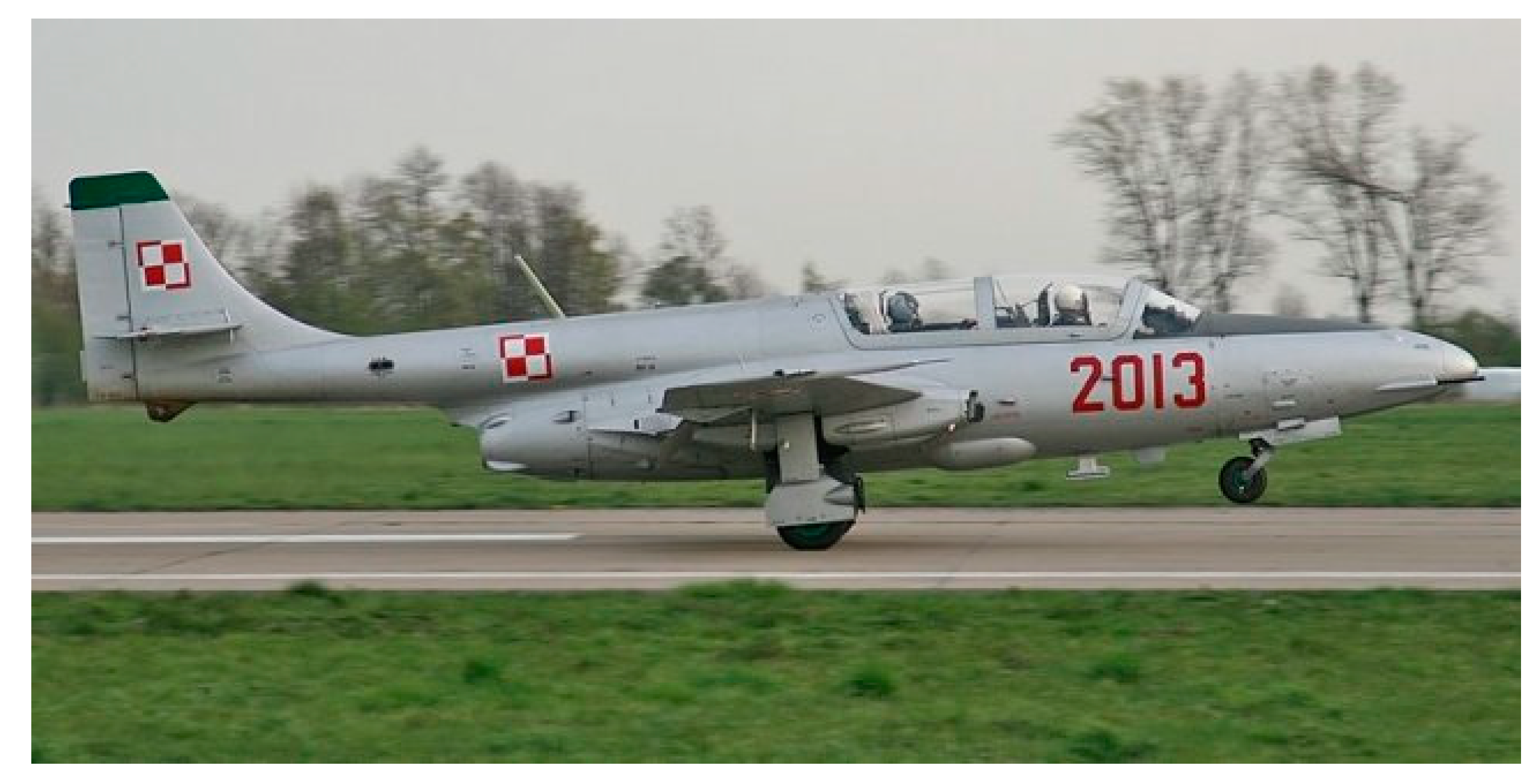
The TS-11 “ISKRA” is a single-engine, jet-powered, two-seat training aircraft designed for:

• initial training;
• aerobatic training;
• instrument flying;
• training in shooting and bombing;
• recognition and photography of objects.

It should be mentioned that the TS-11 aircraft is equipped with the NS-23KM or NR-23 cannon (depending on the equipment version), the ASP-3NM-1 target sight and the S-13 photo cannon. Moreover, additional armament such as bombs weighing up to 100 kg can be mounted on four suspension nodes under the wings.

At present, the Polish Air Force is the only military user of the TS-11 aircraft, however, the quality of the design may be proved by the fact that in 1975, 50 units of the aircraft were ordered by the Indian Air Force. India was a user of “Iskra” until 16 December 2004, and during the entire period of its exploitation, in total 76 TS-11s were used.

2.2. Process of Aircraft Operation

The TS-11 Iskra aircraft has been operated in the Polish Air Force since the 1960s. The years of use allowed for perfect familiarization with the equipment and all the secrets of its operation, which enables efficient and effective conduct of all work and, as a result, safe execution of all anticipated air operations.

The main works carried out on the analyzed aircraft are:

• preliminary maintenance- conducted every 7(+3) flight hours, every two flight shifts or 10(+/−2) days of downtime;
• Pre-flight services, carried out before each first flight shift departure;
• Pre-flight services, carried out before each first flight shift departure—take-off services, carried out before each departure;
• Flight services, conducted after the last flight of the day;
• monthly services.

Moreover, every aircraft TS-11 requires carrying out works resulting from unexpected failures caused by random events such as for example, collisions with birds or excessive wear of operational parts.

Conducting meticulous technical maintenance allows reliable operation of all aircraft sub-assemblies to be ensured and consequently, safe performance of tasks by the flying personnel.

3. Methods

3.1. Markov Processes

Markov processes are one of the most important classes of stochastic processes. They allow the description and analysis of real events and random processes.

With the help of stochastic processes it is possible to describe the variability of random quantities in the analysed period of time in a mathematical way. A real application of the described processes may be, for example, the analysis of time-varying operational states of aircraft of a specific military unit.

Assuming that “T” denotes the set of real numbers $ℝ$, stochastic (random) process can be called a group $\{X_t:tϵT\}$ of real random variables defined in a common probability space with values belonging to the set S $\subset ℝ$.

A random process $\{X_t:tϵT\}$ called a Markov process when the set of states S is finite or recalculable and, moreover, for any i, j, i₀, i₁, …, i_n−1 $ϵ$ S and also t₀, t₁, …, t_n, t_n+1 $ϵ$ $ℝ$+ such that 0 ≤ t₀ < t₁ < … t_n < t_n+1 the formula [14]:

$$P\left(X_{t_{n+1}}=j|X_{t_n}=i,X_{t_{n-1}}=i_{n-1},\dots ,X_{t_1}=i_{1,}{X}_{t_0}=i_0\right)=P(X_{t_{n+1}}=j|X_{t_n}=i)$$

is valid.

When moment t_n+1 is interpreted as a future moment, t_n as a present moment and t₀, t₁, …, t_n, t_n−1 1 as past moments, it can be seen that a characteristic of Markov processes is that, knowing the present state of the process, the distribution of future states does not depend on past processes.

A Markov chain can be called such a Markov process which is a sequence of random variables in which the set of parameters T is identical to the set of natural numbers N₀ = {0, 1, 2, …}.

One can speak of Markov processes with “continuous time” when y T = $ℝ$+.

This is when the formula:

$$P\left(X_{t_{n+1}}=j|X\left(t_n\right)=i)\right)=P(X_{t_{n+1}-t_n}=j|X_0=i)=p_{ij}(t_{n+1}-t_n)$$

is valid for any i, j $ϵ$ S as well as t_n, t_n+1 $ϵ$ ${ℝ}_{+}$ such that 0 ≤ t₀ < t_n+1, the Markov process under analysis is homogeneous.

Assuming that $t=t_{n+1}-t_n$:

$$p_{ij}\left(t\right)=P\left(X_t=j|X_0=i\right),i,jϵ\mathrm{S}t\ge 0$$

The above formula defines the probability of transition from state i to state j after time t.

The definition of a homogeneous Markov process with a discrete state space allows us to specify the assumptions described by the formulas:

$$p_{ij}\left(t\right)\ge 0,t\ge 0$$

$${\displaystyle \sum }_{i\in S}{p}_{ij}\left(t\right)=1$$

$$p_{ij}\left(t+s\right)={{\displaystyle \sum }}_{k\in S}{p}_{ik}\left(t\right)p_{kj}\left(s\right),t\ge 0,s\ge 0$$

The last equation is called Smoluchowski–Chapman–Kolmogorov.

In the case under consideration, the intensity of process transitions is also important. For any homogeneous Markov process, there are always limits according to the formula:

$${\lambda }_i=\underset{h\to 0^{+}}{\lim }\frac{1-p_{ij}\left(h\right)}{h}\le \infty ,\mathrm{where}iϵ\mathrm{S}$$

moreover, there are finite limits described by the equation:

$${\lambda }_{ij}=\underset{h\to 0^{+}}{\lim }\frac{p_{ij}\left(h\right)}{h}=p_{ij}\left(0\right)<\infty ,i,jϵ\mathrm{S},\mathrm{where}i\ne j$$

The probabilities of a change of state can be written in the form of a likelihood matrix using the formula:

$$P\left(t\right)=\left[p_{ij}\left(t\right)\right],i,jϵ\mathrm{S},$$

However, it can be assumed that for each $t>0$ it is a stochastic matrix.

$$p_{ij}\left(0\right)=\{\begin{array}{c}1, for i=j\\ 0, for i\ne j\end{array}$$

The transition intensity matrix can characterize any homogeneous Markov process with a finite state space S = {1, 2, …, r}.

$$A=\left[\begin{array}{cccc}-{\lambda }_1& {\lambda }_{12}& \dots & {\lambda }_{1r}\\ {\lambda }_{21}& -{\lambda }_2& \dots & {\lambda }_{2r}\\ ⋮& ⋮& \ddots & ⋮\\ {\lambda }_{r1}& {\lambda }_{r2}& \dots & -{\lambda }_r\end{array}\right]$$

Determination of the intensity matrix is possible using a known transition probability matrix, but reversing this process is much more complicated.

The procedure is described by Kolmogorov differential equations:

$$p_{ij}\left(t\right)=-{\lambda }_j{p}_{ij}\left(t\right)+{\displaystyle \sum }_{k\ne j}{\lambda }_{kj}{p}_{ik}\left(t\right)$$

$$p_{ij}\left(t\right)=-{\lambda }_i{p}_{ij}\left(t\right)+{\displaystyle \sum }_{k\ne i}{\lambda }_{ik}{p}_{kj}\left(t\right)$$

The use of Kolmogorov differential equations makes it possible to create a proof that the distribution of a Markov process at time $t>0$ is a solution to a system of differential equations $d\left(t\right)=d\left(t\right)A$ [3].

3.2. Operating State Model

The examination of the readiness of the aircraft to perform air tasks should begin with a strict definition of the operational states in which the aircraft may be located, together with a determination whether these states meet all the readiness conditions.

The TS-11 Iskra aircraft may be in the following states:

• pre-flight service—carrying out a thorough check of the aircraft’s systems together with an extended engine test performed before each flight day (according to the provisions of the “time standards for performing current maintenance” the duration of the service is 45 min);
• Starting service—refueling and replacing operating fluids and checking the airplane by technicians carried out each time before the flight (in accordance with the provisions of the “time standards for current service” the duration of the service is 15 min.);
• Flight—time from starting the engine with the intention of performing the flight task until its shutdown after taxing;
• post-flight maintenance—refueling, fueling and securing of the aircraft, carried out after the last flight of each day (according to the provisions of the “time standards for current maintenance” the duration of the service is 30 min);
• taking over the aircraft by the pilot—checking the efficiency of the aircraft by the pilot each time before performing the flight (the duration of the take-over was determined to be 10 min based on the observation of the pilots’ behavior);
• aircraft malfunction or work carried out at WZL No. 1 in Dęblin;
• waiting time—time when no activities are performed on the aircraft but it is ready to perform flight tasks.

In order to examine readiness, it is necessary to determine which of the above states are indicative of the aircraft’s ability to perform the task. Certainly the states which allow this are pilot takeover and flight.

These are periods when the aircraft is fully operational. For the purpose of this paper, these states are considered as the readiness time because only during these states is the aircraft ready to perform the task immediately or is in the process of doing it.

Moreover, the states during which the aircraft is fully operational, but in order to complete the task it is necessary to perform the work of technicians on the ground (it is not ready for immediate completion of the task), are:

• pre-flight services;
• take-off services;
• in-flight services;
• waiting time.

The only state in which the analyzed aircraft is not ready for flight is the state of aircraft malfunction or work in progress at WZL No. 1 in Dęblin.

In addition to a detailed analysis of the states in which the aircraft may be located, attention should also be paid to the characteristics of transitions between these states (Figure 2).An aircraft being in one of the states including S1, S2, S3, S5 defined as states of readiness, has the ability to transition by jumps to another operating state. It must be specified that state 5 takes place after the pre-flight service and start-up service (before the flight state). The time spent in one state before an aircraft is transitioned to the next state is a random variable. Knowledge of this issue results from expertise or procedures imposing a particular order.

It can be best illustrated by a diagram or a zero-one matrix (

Table 1. The possibility of transitions between certain states (own study).

	λij	S1	S2	S3	S4	S5	S6	S7
S1—pre-flight service	S1	0	1	0	0	0	1	1
S2—start-up service	S2	0	0	0	0	1	1	1
S3—flight	S3	0	0	0	1	0	1	1
S4—post-flight service	S4	0	0	0	0	0	1	1
S5—taking over of the aircraft by the pilot	S5	0	0	1	0	0	1	0
S6—WZL or failure	S6	1	0	0	0	0	0	1
S7—waiting	S7	1	0	0	0	0	1	0

). Due to a large number of states causing the complexity of the scheme, it was decided to present the possibilities of transitions by means of a matrix.

3.3. Readiness of Analysed Objects to Perform an Aviation Task

This shows the possibilities of transitions between states.

The matrix of transitions between states can be described by a system of differential equations:

$$\begin{array}{c}\frac{{\mathrm{dP}}_1\left(\mathrm{t}\right)}{\mathrm{dt}}=-({\mathsf{\lambda }}_{16}+{\mathsf{\lambda }}_{17}){\mathrm{P}}_1\left(\mathrm{t}\right)+{\mathsf{\lambda }}_{21}{\mathrm{P}}_2\left(\mathrm{t}\right)+{\mathsf{\lambda }}_{61}{\mathrm{P}}_6\left(\mathrm{t}\right)+{\mathsf{\lambda }}_{71}{\mathrm{P}}_7\left(\mathrm{t}\right)\\ \frac{{\mathrm{dP}}_2\left(\mathrm{t}\right)}{\mathrm{dt}}=-{\mathsf{\lambda }}_{21}{\mathrm{P}}_2\left(\mathrm{t}\right)+{\mathsf{\lambda }}_{52}{\mathrm{P}}_5\left(\mathrm{t}\right)+{\mathsf{\lambda }}_{62}{\mathrm{P}}_6\left(\mathrm{t}\right)+{\mathsf{\lambda }}_{72}{\mathrm{P}}_7\left(\mathrm{t}\right)\\ \frac{{\mathrm{dP}}_3\left(\mathrm{t}\right)}{\mathrm{dt}}=-{\mathsf{\lambda }}_{35}{\mathrm{P}}_3\left(\mathrm{t}\right)+{\mathsf{\lambda }}_{43}{\mathrm{P}}_4\left(\mathrm{t}\right)+{\mathsf{\lambda }}_{63}{\mathrm{P}}_6\left(\mathrm{t}\right)+{\mathsf{\lambda }}_{73}{\mathrm{P}}_7\left(\mathrm{t}\right)\\ \frac{{\mathrm{dP}}_4\left(\mathrm{t}\right)}{\mathrm{dt}}=-{\mathsf{\lambda }}_{43}{\mathrm{P}}_4\left(\mathrm{t}\right)+{\mathsf{\lambda }}_{64}{\mathrm{P}}_6\left(\mathrm{t}\right)+{\mathsf{\lambda }}_{74}{\mathrm{P}}_7\left(\mathrm{t}\right)\\ \frac{{\mathrm{dP}}_5\left(\mathrm{t}\right)}{\mathrm{dt}}=-{\mathsf{\lambda }}_{52}{\mathrm{P}}_5\left(\mathrm{t}\right)+{\mathsf{\lambda }}_{35}{\mathrm{P}}_3\left(\mathrm{t}\right)+{\mathsf{\lambda }}_{65}{\mathrm{P}}_6\left(\mathrm{t}\right)\\ \frac{{\mathrm{dP}}_6\left(\mathrm{t}\right)}{\mathrm{dt}}=-\left({\mathsf{\lambda }}_{61}+{\mathsf{\lambda }}_{62}+{\mathsf{\lambda }}_{63}+{\mathsf{\lambda }}_{64}+{\mathsf{\lambda }}_{65}+{\mathsf{\lambda }}_{67}\right){\mathrm{P}}_6\left(\mathrm{t}\right)+{\mathsf{\lambda }}_{16}{\mathrm{P}}_1\left(\mathrm{t}\right)+{\mathsf{\lambda }}_{76}{\mathrm{P}}_7\left(\mathrm{t}\right)\end{array}$$

$$\frac{{\mathrm{dP}}_7\left(\mathrm{t}\right)}{\mathrm{dt}}=-\left({\mathsf{\lambda }}_{71}+{\mathsf{\lambda }}_{72}+{\mathsf{\lambda }}_{73}+{\mathsf{\lambda }}_{74}+{\mathsf{\lambda }}_{76}\right){\mathrm{P}}_7\left(\mathrm{t}\right)+{\mathsf{\lambda }}_{17}{\mathrm{P}}_1\left(\mathrm{t}\right)+{\mathsf{\lambda }}_{67}{\mathrm{P}}_6\left(\mathrm{t}\right)$$

where:

• P₁(t)—the probability of the aircraft being in a ‘pre-flight maintenance’ state;
• P₂(t)—the probability of the aircraft being in a “star-up” state;
• P₃(t)—the probability of the aircraft being in the ‘flight’ state;
• P₄(t)—the probability of the aircraft being in a state of “ after flight service”;
• P₅(t)—the probability of the aircraft being in the ‘pilot take-over’ state;
• P₆(t)—the probability of the aircraft being in a state of WZL or failure;
• P₇(t)—the probability of the aircraft being in the ‘waiting’ state;

Probabilities can be determined using Wolfram Mathematica.

4. Results

4.1. Analysis of the Probability of Occurrence Limits in the Different States

The results obtained in the research carried out owing to methods described above are presented below. They refer to average annual time of all the analysed aircraft being in certain states (

Table 2. Average annual time of all the analysed aircraft being in certain states (own study).

	Average Annual Time of Occurrence Duration [min]	Average Duration of One Single Occurrence [h]	Average Number of Occurrences within a Year	Average Annual Time of Occurrence Duration [h]	Average Daily Time of Occurrence Duration [h]
S1—pre-flight service	2351.25	0.75	52.25	39.1875	0.107363
S2—start service	1740	0.25	116	29	0.079452
S3—flight	7653	1.099569	116	127.55	0.349452
S4—post-flight service	1567.5	0.5	52.25	26.125	0.071575
S5—taking over of the aircraft by the pilot	1160	0.166667	116	19.33333	0.052968
S6—WZL or malfunction	309,600	24	215	5160	14.13699
S7—waiting time	201,528.25	24	139.95	3358.804	9.202203
Altogether	525,600			8760	24

); probability of transition between certain exploitation states (

Table 3. Probability of transition between certain exploitation states (own study).

pij	S1	S2	S3	S4	S5	S6	S7
S1	0	0.24631	0.0000	0	0	0.45652	0.29717
S2	0	0	0	0	0.246311	0.45652	0.29717
S3	0	0	0	0.12832	0	0.528	0.34369
S4	0	0	0	0	0	0.60572	0.39428
S5	0	0	0.35045	0	0	0.64955	0
S6	0.27185	0	0	0	0	0	0.72815
S7	0.19551	0	0	0	0	0.80449	0

); intensity of transitions between certain exploitation states, average values for the whole group of objects (

Table 4. Intensity of transitions between certain exploitation states, average values for the whole group of objects. The data below should be interpreted as follows: for instance the data 1.511 means a statistical amount of transitions per day between state S₃ and S₆ (own study).

λij	S1	S2	S3	S4	S5	S6	S7
S1	−9.314	2.294	0	0	0	4.252	2.768
S2	0	−12.586	0	0	3.1	5.746	3.74
S3	0	0	−2.862	0.367	0	1.511	0.984
S4	0	0	0	−13.971	0	8.463	5.509
S5	0	0	6.616	0	−18.879	12.263	0
S6	0.019	0	0	0	0	−0.071	0.052
S7	0.021	0	0	0	0	0.087	−0.109

) and the possibility of aircraft being in all exploitation states (Figure 3).

4.2. Analysis of the Probability of Limit Values in the Different States

Based on the values obtained during the analysis of the operation of the aircraft under study, it is easy to see that the dominant states in the cases described are “expectation” and “WZL or failure”. The other states are only of marginal importance.

In order to calculate the limiting probability of the analysed object being in a certain state of readiness, the following formula should be used:

$$k=\frac{{{\displaystyle \sum }}_{i=1}^y{P}_x}{{{\displaystyle \sum }}_{i=1}^{7}P},$$

where: $P_x$—states of being ready, not ready or not ready, P—any state the aircraft has the possibility to be in.

Knowing that the sum of the probabilities in which an object can be located is always equal to 1 (the denominator of the above formula), it can be determined that the probability of being in a specific readiness state is always equal to the sum of the probabilities of the individual operating states assigned to a given state of readiness. Thus:

• the probability of the analysed objects being in a state of full readiness to perform an aviation task:

$$k_1=P_3+P_5$$

• the probability of analysed objects being in a state of incomplete readiness for a flight task:

$$k_1=P_1+P_2+P_4+P_7$$

• the probability of analysed objects being in a state of unpreparedness for an aerial task:

$$k_1=P_6$$

According to the presented classification it is possible to calculate, that the limiting probability of being in the state of:

• task readiness is: 0.021%;
• not ready to perform the task is: 37.032%;
• ready to perform the task is: 62.946%.

5. Discussion

Conducting an analysis of the operation of the TS-11 “Iskra” aircraft made it possible to show that in spite of the fact that analysed aircraft are exploited in an ineffective way (probability of being in mission readiness states) flights are performed safely and that most of the analysed objects realised planned annual exploitation assumptions.

It has been noted that the high level of training of ground staff affects the safety of flying tasks significantly. On the base of interviews with pilots performing tasks on the TS-11 “Iskra”, one can be sure that they are confident about the proper conduct of ground work and fully trust that the aircraft is always prepared properly to perform the mission. Moreover, opinions of cadets performing flights on transport aircraft indicate that the equipment they use is properly operated.

It should also be highlighted that the presented model is universal and can be used also for various aircraft. Owing to data obtained in a survey, it is possible to calculate how many aircraft may be available and with what probability. An innovation introduced in relation to previously discussed models is the introduction of the state of pilot takeover of the aircraft.

6. Conclusions

To sum up, this publication proposes a method for calculating the readiness of aircraft used by the Armed Forces of the Republic of Poland. The author’s own seven-state descriptive model of the exploitation process was developed for use with complex military objects using the Markov theory. At the same time, it should be noticed that there is still a small number of publications in the field of Markov theory applications relating to the construction and operation of technical facilities particularly in the field of aircraft performance. This enables reliable analysis resulting in determining a statistical availability of the aircraft number. The authors’ contribution to this work is based on the reliability of the empirical tests carried out on TS-11 aircraft and its practical suitability for aviation. What is worth mentioning is the fact of introducing an innovative element considering one more state: taking over an aircraft by a pilot. The mission readiness states are influenced by weather conditions, planned repairs excluding aircraft from the exploitation records, and due to readiness remaining on a low level.

References

- Basora, L.; Bry, P.; Olive, X.; Freeman, F. Aircraft Fleet Health Monitoring with Anomaly Detection Techniques. Aerospace 2021, 8, 103. [Google Scholar] [CrossRef]
- Zurek, J.; Jankowski, A.; Rajchel, J. Analysis of the Aircraft Operation in the Context of Safety and Effectiveness; Gomes, J.F.S., Meguid, S.A., Eds.; Inegi-Feup: Porto, Portugal, 2015; pp. 193–202. ISBN 978-989-98832-3-9. [Google Scholar]
- Zurek, J.; Zieja, M.; Ziolkowski, J. The Analysis of the Helicopter Technical Readiness by Means of the Markov Processes; Gomes, J.F.S., Meguid, S.A., Eds.; Inegi-Inst Engenharia Mecanica E Gestao Industrial: Porto, Portugal, 2018; pp. 1387–1400. ISBN 978-989-20-8313-1. [Google Scholar]
- Tomaszewska, J.; Zurek, J. Analysis of the Equipment Operation System in Terms of Availability. J. KONBiN 2017, 40, 5–20. [Google Scholar] [CrossRef] [Green Version]
- McPherson, J.W. Reliability Physics and Engineering: Time-to-Failure Modeling, 3rd ed.; Springer International Publishing: Berlin/Heidelberg, Germany, 2019; ISBN 978-3-319-93682-6. [Google Scholar]
- Żurek, J. Review of the safety evaluation methods in aviation. Probl. Eksploat. 2009, nr 4, 61–70. [Google Scholar]
- Ntantis, E.L.; Botsaris, P. Diagnostic Methods for an Aircraft Engine Performance. J. Eng. Sci. Technol. Rev. 2015, 8, 64–72. [Google Scholar] [CrossRef]
- Liao, B.; Sun, B.; Li, Y.; Yan, M.; Ren, Y.; Feng, Q.; Yang, D.; Zhou, K. Sealing Reliability Modeling of Aviation Seal Based on Interval Uncertainty Method and Multidimensional Response Surface. Chin. J. Aeronaut. 2019, 32, 2188–2198. [Google Scholar] [CrossRef]
- Yadav, C.S.; Singh, R. Reliability of Object Oriented Systems with Markov Transfer of Control. In Proceedings of the 2011 International Conference on Computer and Management (CAMAN), Wuhan, China, 19–21 May 2011; pp. 1–3. [Google Scholar]
- Zhou, C.; Chang, Q.; Zhou, C.; Zhao, H.; Shi, Z. Fault Tree Analysis of an Aircraft Flap System Based on a Non-Probability Model. Qinghua Daxue Xuebao/J. Tsinghua Univ. 2021, 61, 636–642. [Google Scholar] [CrossRef]
- Diamoutene, A.; Noureddine, F.; Kamsu-Foguem, B.; Barro, D. Reliability Analysis with Proportional Hazard Model in Aeronautics. Int. J. Aeronaut. Space Sci. 2021, 22, 1222–1234. [Google Scholar] [CrossRef]
- Zieja, M.; Ważny, M.; Stępień, S. Outline of a Method for Estimating the Durability of Components or Device Assemblies While Maintaining the Required Reliability Level. EiN 2018, 20, 260–266. [Google Scholar] [CrossRef]
- Rudnicki, J. Comparative Analysis of Results of Application of Markov and Semi-Markov Processes to Reliability Models of Multi-State Technical Objects. J. Pol. CIMEEAC 2016, 1, 169–181. [Google Scholar]
- Grabski, F. Markov and Semi-Markov Processes as a Failure Rate. AIP Conf. Proc. 2016, 1738, 480012. [Google Scholar] [CrossRef]