Mechanism and Performance Differences between the SSG/LRR-ω and SST Turbulence Models in Separated Flows

Abstract

Accurate predictions of flow separation are important for aerospace design, flight accident avoidance, and the development of fluid mechanics. However, the complexity of the separation process makes accurate predictions challenging for all known Reynolds-averaged Navier–Stokes (RANS) methods, and the underlying mechanism of action remains unclear. This paper analyzes the specific reasons for the defective predictions of the turbulence models applied to separated flows, explores the physical properties that impact the predictions, and investigates their specific mechanisms. Taking the Menter SST and the Speziale-Sarkar–Gatski/Launder–Reece–Rodi (SSG/LRR)-ω models as representatives, three typical separated flow cases are calculated. The performance differences between the two turbulence models applied to the different separated flow calculations are then compared. Refine the vital physical properties and analyze their calculation from the basic assumptions, modeling ideas, and construction of the turbulence models. The numerical results show that the underestimation of Reynolds stress is a significant factor in the unsatisfactory prediction of separation. In the SST model, Bradshaw’s assumption imposes the turbulent energy equilibrium condition in all regions and the eddy–viscosity coefficient is underestimated, which leads to advanced separation and lagging reattachment. In the SSG/LRR-ω model, the fidelity with which the pressure–strain term is modeled is a profound factor affecting the calculation accuracy.

1. Introduction

Flow separation is a significant and complex problem in fluid dynamics. For aircraft, excessive separation will cause lift reduction, drag increment, and even stall, which affects both flight stability and structural safety. Therefore, accurate separation predictions are crucial to the design and optimization of aircraft [1]. However, all known turbulence models struggle to predict separated flows accurately because of the existence of large adverse pressure gradients near the separation area and complex flow structures, such as separation bubbles [2] and vortices in the reverse-flow region.

The commonly used turbulence models can be divided into two main categories: eddy–viscosity models (EVMs) and Reynolds–stress models (RSMs). EVMs follow the Boussinesq approximation and introduce the eddy–viscosity coefficient to close the Reynolds stress, whereas RSMs are derived strictly from the Navier–Stokes equations and solve the Reynolds stress directly. The economy, robustness, and clarity of their performance characteristics have made EVMs popular for industrial design. However, for some complex flows, EVMs have inherent unavoidable defects, such as isotropy and the instantaneous balance between the Reynolds stress tensor and the average strain rate [3]. RSMs reflect the physical mechanism of turbulence more directly and accurately. They outperform EVMs when applied to separated flows, rotating flows, and corner secondary flows. However, their advantages over the traditional EVMs are not overwhelming [3]. There are still cases where some EVMs perform better than RSMs. Therefore, it would be of great benefit to the development of turbulence models to analyze the fundamental reasons for the performance differences between RSMs and EVMs. As highlighted in the CFD Vision 2030 Study [4], it is important to undertake sufficient research on the RSM framework so as to further develop its potential.

Many researchers have conducted numerical simulations of separated flows. In studying a rearward-facing step in a diverging channel flow, Driver et al. [5] found a large deviation between the results predicted by the turbulence model and the experimental values for the reattachment process. Zhao et al. [6] studied supersonic flows past 2D compression ramps, and found that the Spalart–Allmaras (SA) and SST models gave slightly higher pressures in the separation area compared with experimental data, but the local skin-friction coefficient after reattachment was lower than the experimental value. As the separation area increases, the adaptability of each turbulence model was found to be different. Eisfeld et al. [7] focused on shock-induced separation in transonic flow over an axisymmetric bump, whereby the adverse pressure gradients induced separation in the subsonic flow around the NACA 4412 airfoil at α = 13.87°. They found that the prediction results of the SA and SST models indicate an upstream onset of separation and downstream reattachment, with a longer separation bubble. Although the SSG/LRR-ω model faced similar problems, the predicted results were closer to the experimental values. Bush et al. [8] found that the phenomenon of lagging reattachment may be related to the underestimation of the shear stress in the shear layer above the reverse-flow region. Rumsey et al. [9] found that non-linear effects are important when computing corner flows. Computations on the NASA Common Research Model revealed that the SST model produces large wing–root corner separation bubbles, contrary to experimental evidence, whereas the WilcoxRSM-w2006 and SSG/LRR-RSM-w2012-SD models yield very small bubbles. This is because RSMs can predict the difference among the normal stresses, but two-equation models cannot.

However, previous research has mainly focused on the problems that exist in predictions of the flow structure of the separated flow. Not too many researchers have explored the underlying defects of the turbulence models that may cause the mismatch between the predicted Reynolds stress and the real value when closing the system of equations. Exploring the reasons for defective predictions in separated flows from the perspective of model construction provides a deeper physical understanding of separated flows and may lead to the development of more complete turbulence models.

The remainder of this paper is organized as follows. Section 2 discusses a representative RSM and EVM. Three turbulent separated flows and their calculation results are presented in Section 3. According to the performance differences of the different models, an in-depth analysis is carried out covering the basic assumptions, modeling ideas, and construction of the turbulence models, and a discussion of the respective mechanisms is given in Section 4. The main conclusions from this study are summarized in Section 5. Overall, this paper provides a detailed analysis of the problems with existing turbulence models. It is hoped that this contribution will enable improvements to be made in the future.

2. Turbulence Models

Among the two-equation models, the $k-\epsilon$ and $k-\omega$ models have their own advantages in terms of turbulence predictions. Menter [10] connected them with a blending function to develop the SST model, which combines their respective advantages. The SST model retains the characteristics of the $k-\omega$ model near the wall and the characteristics of the $k-\epsilon$ model at the edge of the boundary layer and in the free shear layer [11]. Due to its excellent robustness, accuracy, and broad applicability, the SST model has been highly evaluated and praised in industry and academia [2,12]. The SST model equations can be found in [13].

In 2005, Eisfeld et al. [14] drew on Menter’s idea and method of constructing the SST model, and combined the LRR model with the SSG model to construct a robust RSM, namely the SSG/LRR-ω model. This model retains the advantages of the LRR model in the area away from the wall, but considers the wall effect on the Reynolds stress distribution as in the SSG model. In this regard, it is similar to the SST model. Rumsey et al. [7] pointed out that the SSG/LRR-ω model is currently the most recommended RSM. Eisfeld, Rumsey, and others have also performed extensive verification and validation on this model [7]. The detailed equations can be found in [7].

The similar construction ideas of the SST and SSG/LRR-ω models enable unnecessary interference to be eliminated as much as possible in the process of comparative analysis. Hence, a rigorous comparison of these turbulence models can be carried out.

3. Case Descriptions and Calculation Results

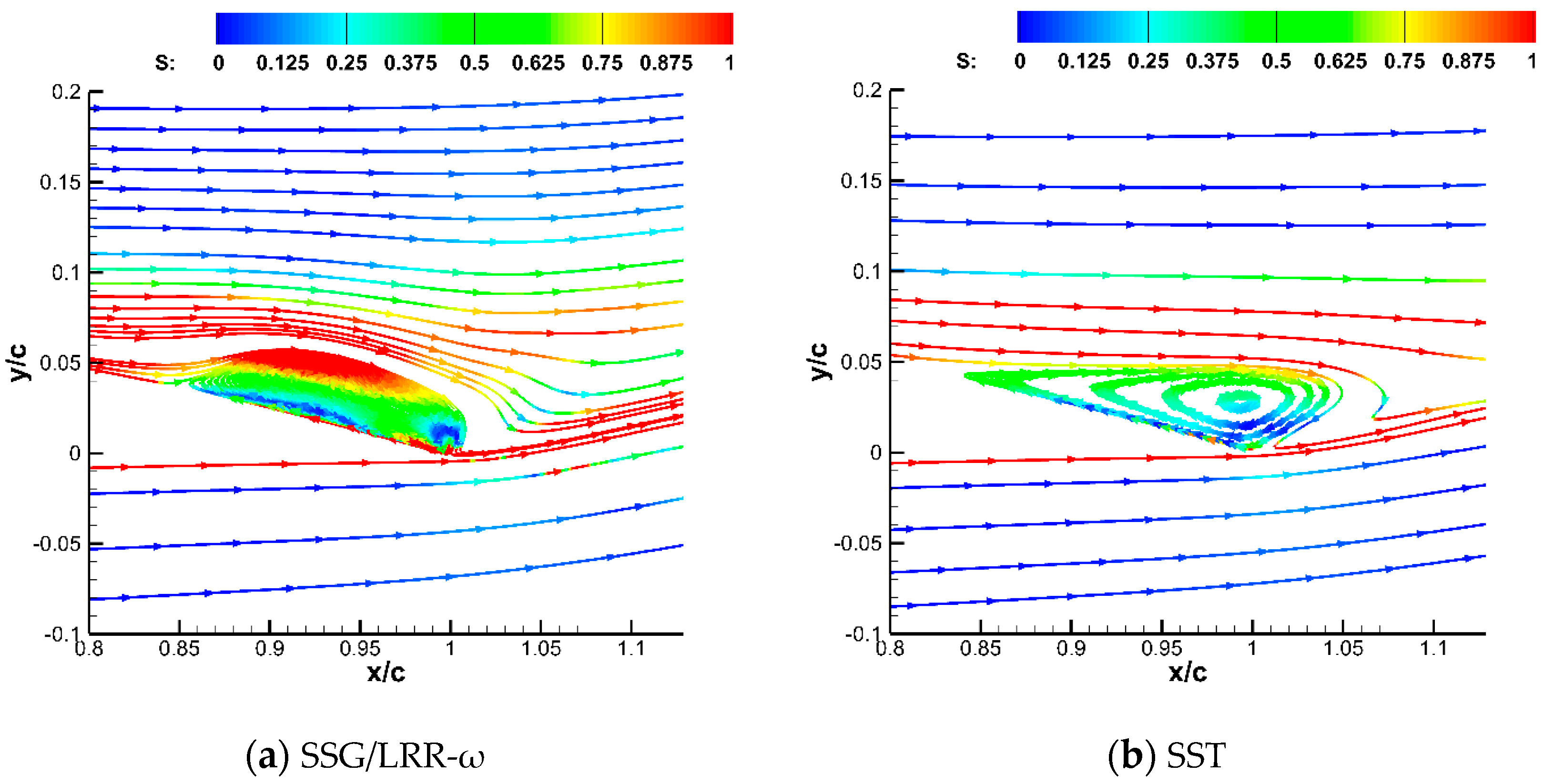
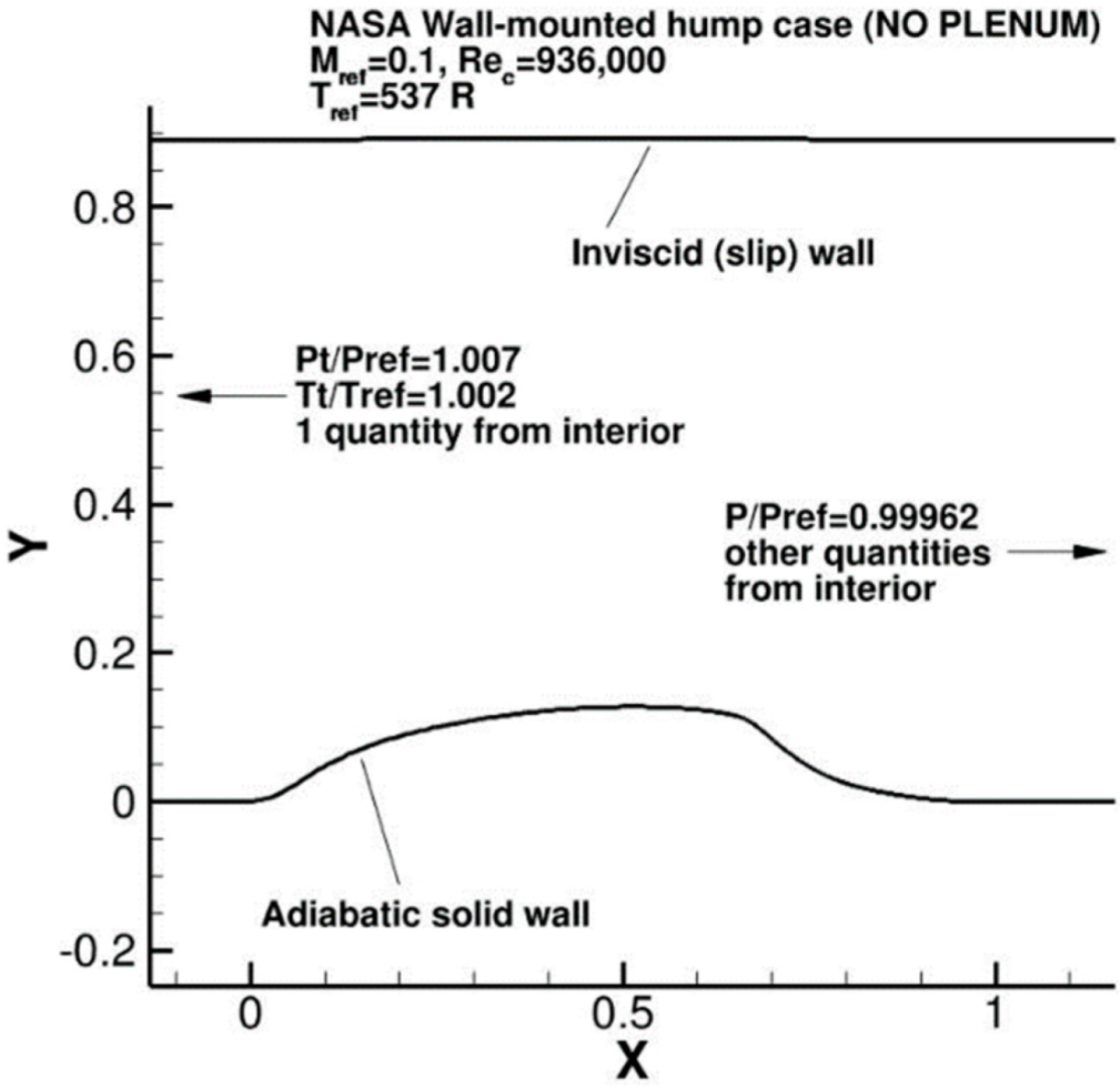
3.1. Two-Dimensional NASA Wall-Mounted Hump Separated Flow

3.1.1. Case Description

The main purpose of this case is to assess the ability of the turbulence models to predict the separation caused by an adverse pressure gradient, the formation of a separation bubble in the separation region, and the subsequent reattachment process [15,16]. Numerical simulations were performed using the structured mesh with a grid resolution of 817 × 217 (flow direction × normal direction). Encryption is carried out near the hump and wall to ensure the capture of the complex flow field structures. The geometry of the hump and boundary conditions are indicated in Figure 1. In this paper, CFL3D [17] is selected for calculation, which is a Reynolds-averaged thin-layer N–S flow solver for structural grids. Its calculation results are widely recognized by international CFD researchers.

3.1.2. Calculation Results

Figure 2 shows the skin-friction distributions predicted by the SSG/LRR-ω model and the SST model and compares them with the experimental results reported by Greenblatt [18]. The separation onset and reattachment point calculated by the two models can be obtained from the curves of the skin-friction coefficient, as presented in

Table 1. Calculation results of separation zone given by SST model and SSG/LRR-ω model.

	Exp. Data	SSG/LRR-ω	SST
Separation onset	0.665	0.654	0.654
Error	——	1.65%	1.65%
Reattachment point	1.1	1.183	1.269
Error	——	7.5%	15.36%

. Both the SSG/LRR-ω and SST models predict the separation onsets to be upstream of the experimental position, while the reattachment occurs downstream. Comparing the calculation results of the two models, it is clear that the separation zone predicted by the SST model is too large, and the reattachment points exhibit serious lag.

The calculated streamlines colored according to the stream-wise velocity are shown in Figure 3. Intuitively, the flow cannot overcome the adverse pressure gradient, and thus separates after passing through the hump. A reverse-flow region forms and separation bubbles are produced, before the flow attaches to the wall.

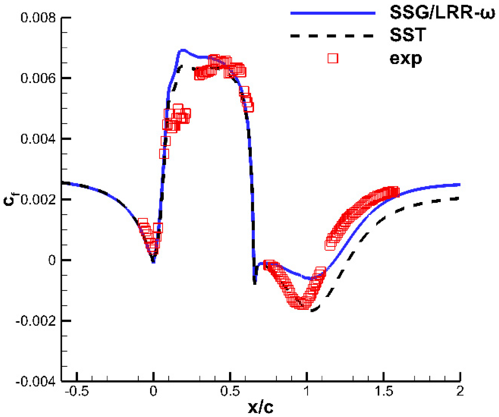
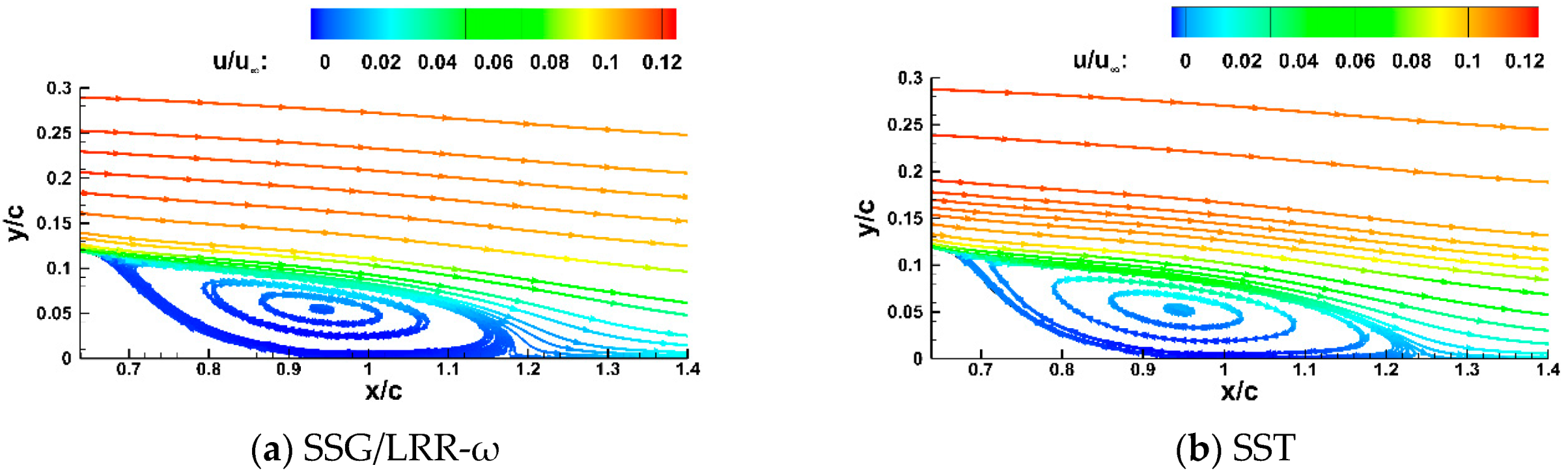
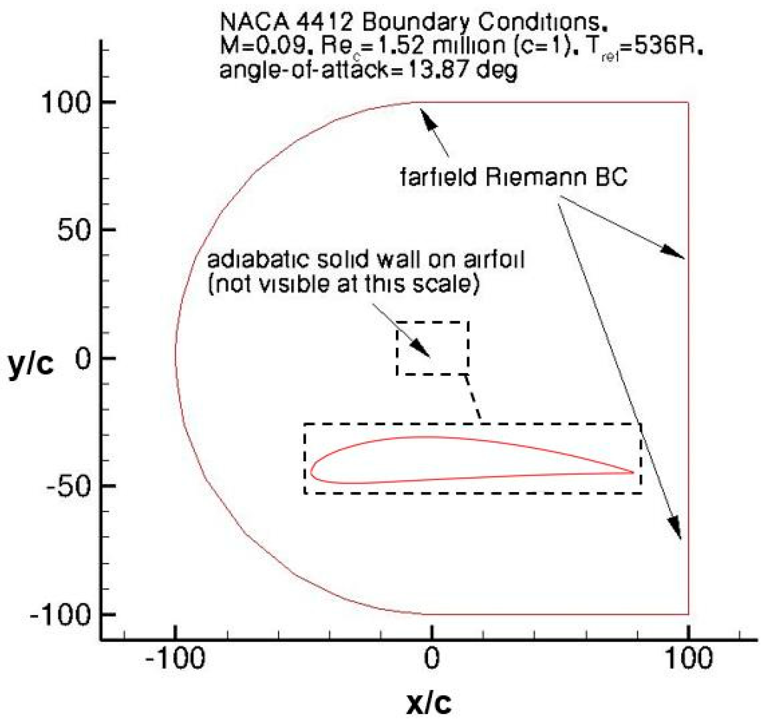
3.2. Subsonic Flow around the NACA 4412 Airfoil

3.2.1. Case Description

The NACA 4412 airfoil with upper surface trailing edge separation examines a model’s ability to reproduce the real physics. Numerical predictions were carried out on the structured mesh with a grid resolution of 257 × 81. The boundary conditions in this calculation case are shown in Figure 4. The incoming flow Mach number is 0.09, the Reynolds number Re_c = 1.52 × 10⁶ (_c is the airfoil chord length), the reference temperature is 297.78 K, and the angle of attack is 13.87°.

3.2.2. Calculation Results

The skin-friction coefficient distribution is shown in Figure 5. The separation onset calculated by the SST model is located at 75% of the chord length, whereas the SSG/LRR-ω model gives a location of 77% of the chord length and the SA model gives a location of 79% of the chord length. In the recirculation area, the $c_f$ value calculated by the SSG/LRR-ω model is slightly smaller than that of the SST model, which is consistent with its performance in the other two calculation cases. This also means that in the calculation results of SSG/LRR-ω, the velocity in the recirculation area is smaller. The calculated streamlines colored according to stream-wise velocity are shown in Figure 6. The separation bubble calculated by the SST model is closer to the real flow, but the calculation result of the SSG/LRR-ω model is slightly worse.

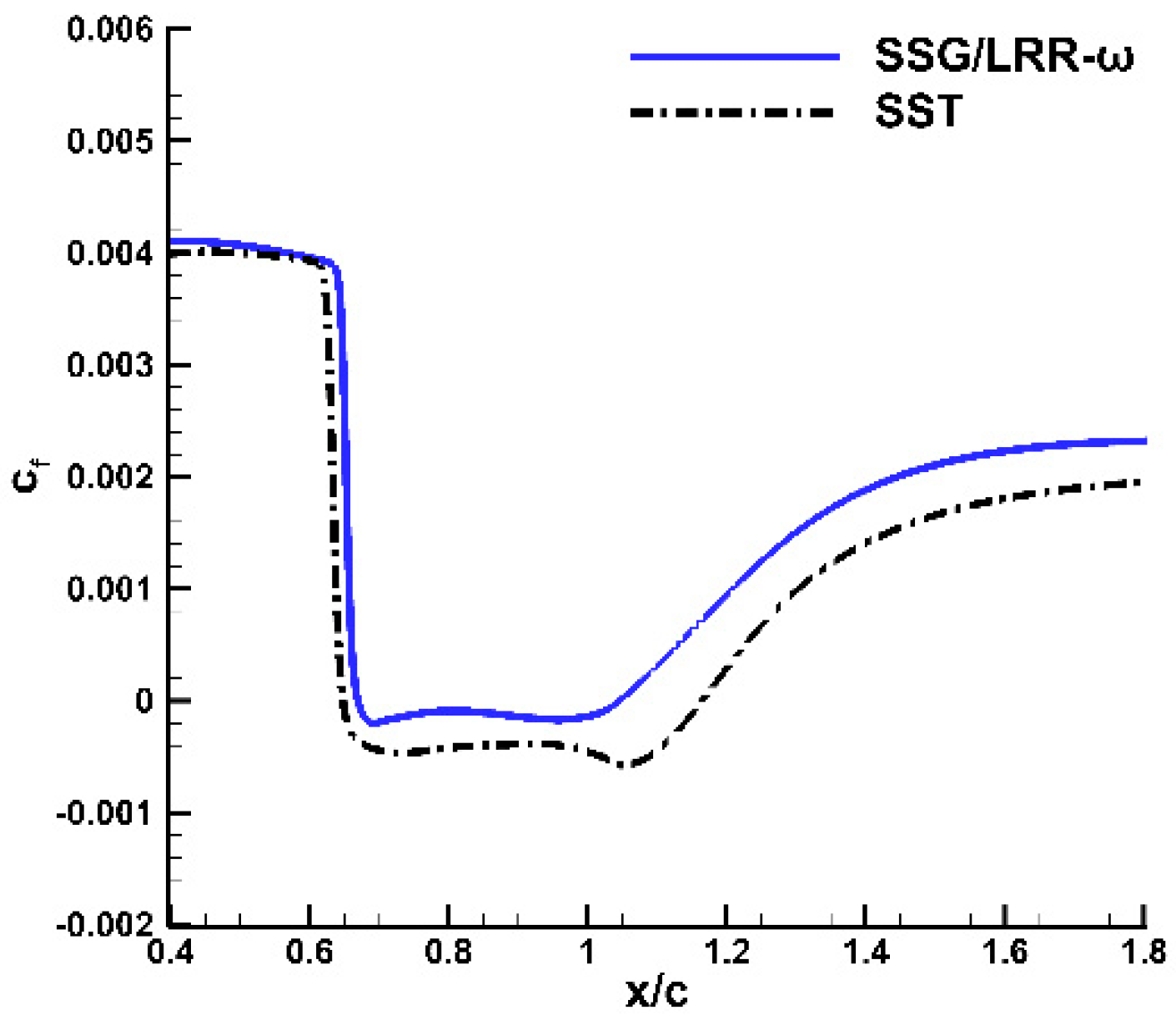
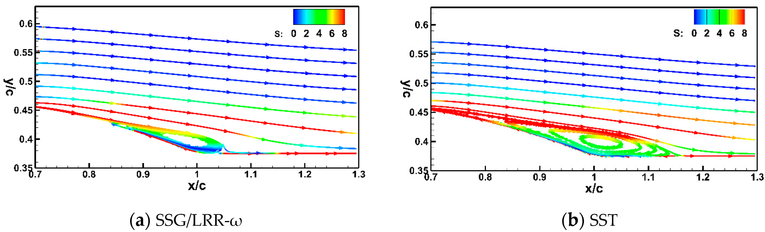
3.3. Axisymmetric Transonic Bump

3.3.1. Case Description

At transonic speeds, the prediction of separated flows is challenging. Alber et al. [19] placed a 2D circular-arc model on the ground to generate a transonic flow field. The experiment showed that when overcoming an adverse pressure gradient, the flow near the wall is very likely to have lateral movement, resulting in changes in the appearance of the entire flow field. When there is a shock wave in the flow field, it is particularly difficult to predict the shock-induced separation accurately. Therefore, the axisymmetric transonic bump is selected to examine the performance of the SSG/LRR-ω and SST models in shock-induced separated flow.

The geometric shape of the model is a 1.905 cm-high and 20.32 cm-long arc-shaped bump nested in the middle of an axisymmetric cylinder of diameter 15.24 cm. The characteristic length is the length of the arc-shaped bump, i.e., c = 20.32 cm, and the bump is located from x/c = 0 to x/c = 1. When the fluid flows over the bump, a shock wave will be generated. Separation occurs downstream of the shock wave, and then the flow reattaches downstream of the bump. Figure 7 shows a sketch of the computational domain. The numerical computations were carried out on the structured grid containing N = 721 × 321 grid points.

3.3.2. Calculation Results

The distributions of the skin-friction coefficient are shown in Figure 8, from which the separation onset and reattachment point calculated by the two models can be obtained (

Table 2. Calculation results of separation zone given by SST model and SSG/LRR-ω model.

	Exp. data	SSG/LRR-ω	SST
Separation onset	0.7	0.67	0.647
Error	——	4.29%	7.57%
Reattachment point	1.1	1.05	1.165
Error	——	4.54%	5.91%

). Both the SSG/LRR-ω and SST models give the onset of separation to be upstream of the experimental values, but the SST model gives a larger error. The SSG/LRR-ω model predicts the reattachment occurring slightly upstream of the experimental value, while the SST model gives a reattachment point downstream of the actual position. The separation area is overestimated by the SST model. Overall, the prediction effect of the SSG/LRR-ω model is better, and the separation bubble length is close to the experimental value.

The calculated streamlines colored according to stream-wise velocity are shown in Figure 9. It is clear that the separation area predicted by the SST model is too long, and the reattachment point exhibits serious lag.

4. Analysis of Differences in Model Performance and Mechanism Exploration

In Section 3, the simulations of separated flows showed that the SST model predicts the onset of separation to be upstream and the reattachment point to be downstream of the experimental positions, resulting in overestimations of the separation area. The results from the SSG/LRR-ω model predict the separation to occur upstream of the experimental value, with some reattachment points upstream and others downstream of the actual position. However, the separation area is in better agreement with the experimental values than that of the SST model.

Actually the performance of the two models is not bad, with the separation points being a few percent off the experimental, and the reattachment points being off somewhat more, but all within what is accepted as usual in turbulence modelling. This may be because the flow structure is simpler in calculation, in more complex flow separation, (such as inlet and wing-body combination of wing root), there will be a greater bias, and even the basic flow structures are predicted to be inconsistent by different turbulence models, which is unacceptable for designers. Therefore, it is necessary to study the causes of the error and try to reduce it.

The next section analyzes the physical reasons for advanced separation and lagging reattachment in the separated flows. We attempt to ascertain the related physical properties and study the difference in performance in terms of the construction principles of the SST and SSG/LRR-ω models.

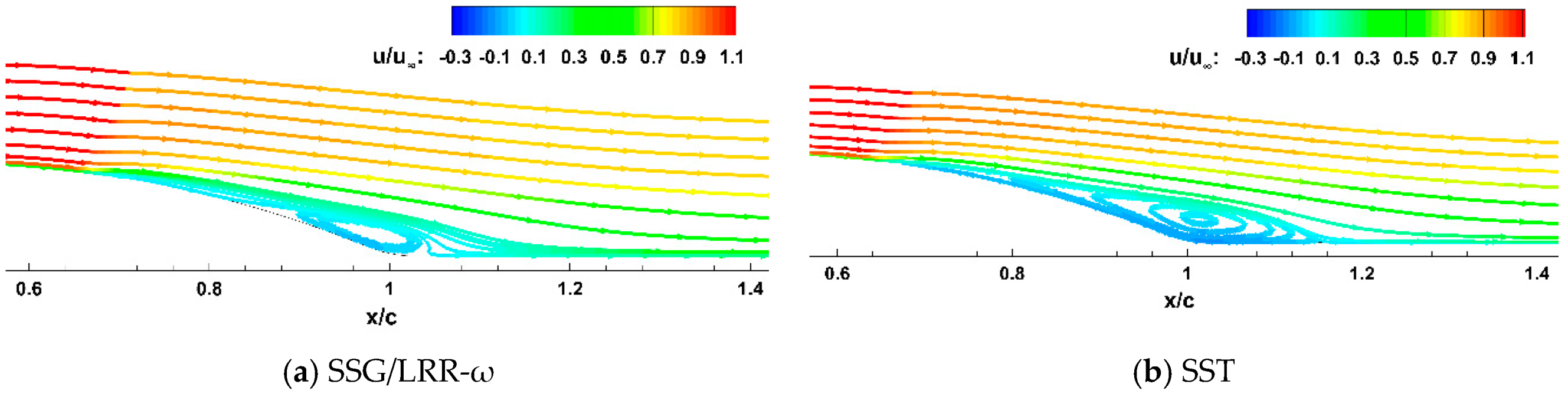
4.1. Advanced Separation

4.1.1. Separation Mechanism and Critical Physical Properties

Separation refers to the phenomenon whereby the boundary layer is no longer attached to the wall, and moves away from the wall and into space due to the influence of viscosity and an adverse pressure gradient. In the turbulent boundary layer, the velocity profile is fully developed. The velocity and momentum exchanges between the upper and lower layers are more intense than in laminar flow. The shear force is more potent, the turbulence fluctuations are greater, and the Reynolds shear stress is larger. However, in the separation region, momentum exchange becomes weaker due to the greatly reduced shear action, and the Reynolds shear stress decreases to a certain extent compared with that before separation. Therefore, if the reduction in the Reynolds shear stress is taken as the criterion for entering the separation zone, the Reynolds stress in the separation zone as calculated by the turbulence model should be lower than that measured experimentally at the corresponding position, and so the separation point should advance.

In turbulent flow, the Reynolds shear stress will be two orders of magnitude larger than the molecular viscous stress [1]. Thus, the molecular viscous stress can be neglected, except for the area extremely near the wall region, i.e.,

$$\tau =\mu \frac{dU}{dy}-\rho \overline{uv}\approx -\rho \overline{uv}$$

(1)

The Reynolds stress at the key station in the hump case is compared with the experimental value in Figure 10. The Reynolds stress calculated by the SST and SSG/LRR-ω models near the separation zone is lower than the experimental value; in particular, the result of the SST model is much lower than the experimental value. Leschziner [20], Eisfeld [7], and Rumsey [16] have all come to similar conclusions in their studies, but simply state that the shear stress is underestimated. This paper attempts to determine the precise reasons for this problem.

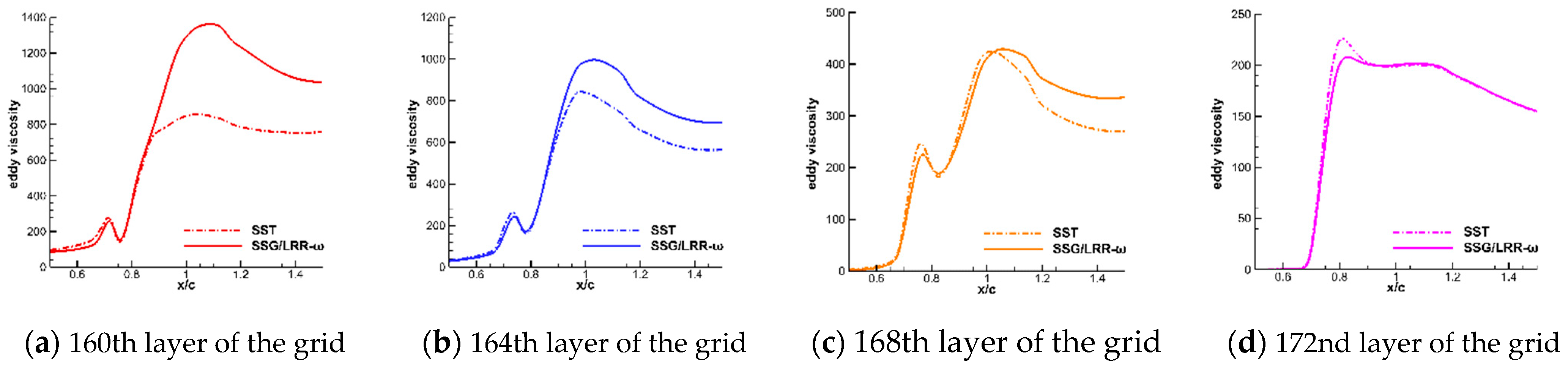
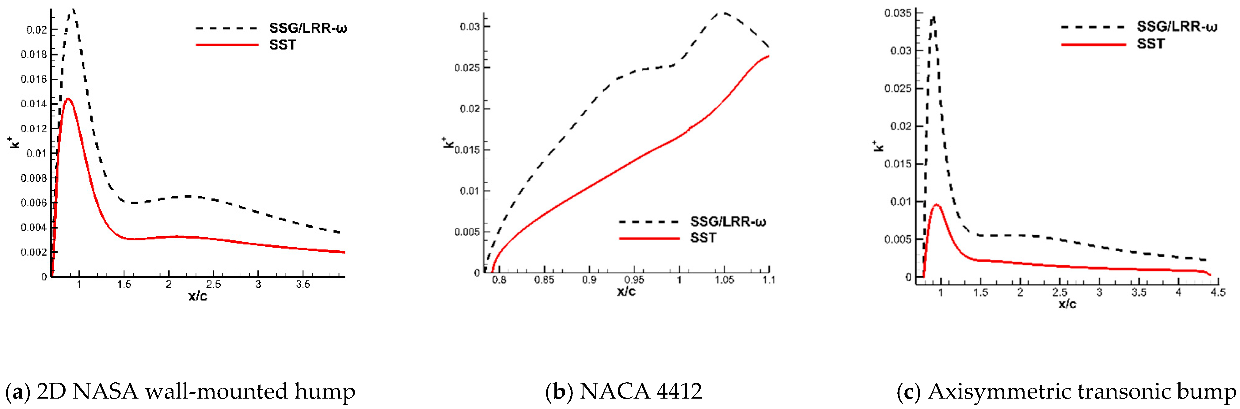
4.1.2. Reasons for Underestimating Shear Stress in the SST Model

According to the above analysis, the molecular viscous stress need only be considered near the wall, and only the Reynolds stress needs to be considered in other places. The SST model is an EVM, and all EVMs are based on the Boussinesq eddy–viscosity approximation, i.e.,

$$-\overline{u_i{u}_j}=2{\nu }_t{S}_{ij}-\frac{2}{3}k{\delta }_{ij}.$$

(2)

Before the development of the SST model, the $k-\epsilon$ model used the following methods to calculate the Reynolds stress:

$$-\overline{\mathit{uv}}=C_{\mu }\frac{k^2}{\epsilon }\left(\frac{\partial U}{\partial y}\right).$$

(3)

The production term is

$$P_k=-\overline{uv}\frac{\partial U}{\partial y}.$$

(4)

Substituting Equation (4) into Equation (3), the shear stress arises as:

$$-\overline{\mathit{uv}}=C_{\mu }{}^{\frac{1}{2}}\sqrt{\frac{P_k}{\epsilon }}k.$$

(5)

One of the main differences between the EVMs and RSMs is that the latter account for the significant effect of the transport of the turbulent shear stress. The success of the Johnson–King model indicated the importance of this term [10], and introduced Bradshaw’s assumption into the modeling of the turbulent shear stress. A linear relationship can be established between the shear stress and the turbulent kinetic energy:

$$-\overline{\mathit{uv}}=\rho {\mathrm{a}}_{1}k.$$

(6)

In cases which have a region with a large adverse pressure gradient, e.g., separated flows, the production term of turbulent kinetic energy is much larger than the dissipation term, $P_k\gg \epsilon$ [10], and the calculated Reynolds stress is usually overestimated compared with Bradshaw’s relation, so the calculation of separated flows is always unsatisfactory. In 1993, Menter developed the SST model based on the $k-\epsilon$ and $k-\omega$ models, and modified the eddy–viscosity coefficient as follows:

$${\nu }_t=\frac{a_{1}k}{\mathit{max}\left(a_1\omega ,S{F}_2\right)}.$$

(7)

In the boundary layer, $F_2\to 1$, and so

$${\nu }_t=\frac{a_{1}k}{\mathit{max}\left(a_1\omega ,S{F}_2\right)}\Rightarrow {\nu }_t=\frac{a_{1}k}{\mathit{max}\left(a_1\omega ,\frac{\partial U}{\partial y}\right)}.$$

(8)

When the two terms in the denominator are equal,

$$a_1\omega =\frac{\partial U}{\partial y}\Rightarrow a_1=\frac{k}{\epsilon }\frac{\partial U}{\partial y}=\frac{{\nu }_t}{k}\frac{\partial U}{\partial y}=-\frac{\overline{uv}}{k}.$$

(9)

That is, corresponding to Bradshaw’s assumption, the Reynolds stress and the turbulent kinetic energy have a linear relationship, which is consistent with the turbulent energy equilibrium: for a thin shear flow, the turbulent kinetic energy production term is approximately equal to the dissipation term in the completely turbulent layer, where the diffusion term tends to zero, and the turbulent energy is balanced [1,21]. Then,

$$\begin{array}{ll}{P}_k=-\overline{\mathit{uv}}\frac{\partial U}{\partial y}=\epsilon & \left(a\right)\\ -\overline{\mathit{uv}}={\nu }_{\mathrm{t}}\frac{\partial U}{\partial y}=C_{\mu }\frac{k^2}{\epsilon }\frac{\partial U}{\partial y}& \left(b\right)\end{array}\}\Rightarrow C_{\mu }={\left(\frac{\overline{\mathit{uv}}}{k}\right)}^2=a_1^2,$$

(10)

where $C_{\mu }=0.09$. When the strain is larger,

$${\nu }_t=\frac{a_{1}k}{\mathit{max}\left(a_1\omega ,S{F}_2\right)}=\frac{a_{1}k}{S},$$

(11)

$$-\overline{uv}={\nu }_{t}S=a_{1}k.$$

(12)

The limiter’s action makes the eddy–viscosity coefficient in the SST model satisfy Bradshaw’s assumption throughout the boundary layer. After introducing this assumption, the Reynolds stress is effectively reduced in highly strained flows compared with Equation (5), and this plays a significant role in promoting separation. However, in the calculated results described above, separation always occurs in advance. Thus, it is necessary to explore the reason behind this phenomenon. The problem still lies with Bradshaw’s assumption. The coefficient ${\mathrm{a}}_1$ in Bradshaw’s relation is only strictly valid in the log layer. The equilibrium mechanism of the equations in other regions is different. For example, in the laminar sublayer, the equilibrium is mainly between the dissipation and diffusion terms, while in the outer layer, it is mainly between the dissipation and convection terms. Nevertheless, Bradshaw et al. suggested that this should be used more generally because other thin shear flows show a similar behavior (albeit with a lower constant) [20].

When the turbulence model is used for simulations, it is impossible to distinguish whether the current calculation region is in the log layer or not. Thus, the coefficient $a_1=0.3$, which is only valid in the log layer, is used in the whole calculation region. When encountering a large adverse pressure gradient, $P_k\gg \epsilon$, part ($a$) in Equation (10) is not valid; when the strain rate is high, vortex stretching will generate additional turbulent kinetic energy, which also makes part ($a$) invalid. In both cases, Equation (10) cannot be obtained; namely, the calculation accuracy of the turbulent model is greatly challenged. Among the three examples calculated in Section 2, the adverse pressure gradient and strain rate are significantly higher in the axisymmetric transonic bump case. Hence, the calculated error is also larger.

The above analysis indicates that Bradshaw’s relation forces the model to impose the condition $P_k=\epsilon$. Although this has a favorable promotion effect on the prediction of separation, this assumption is somewhat harsh. Apsley and Leschziner [22] and Liou [23] pointed out that the SST model is too sensitive in some subsonic, transonic, and supersonic separation flows, leading to separation occurring upstream of the exact position and producing a more extended separation zone.

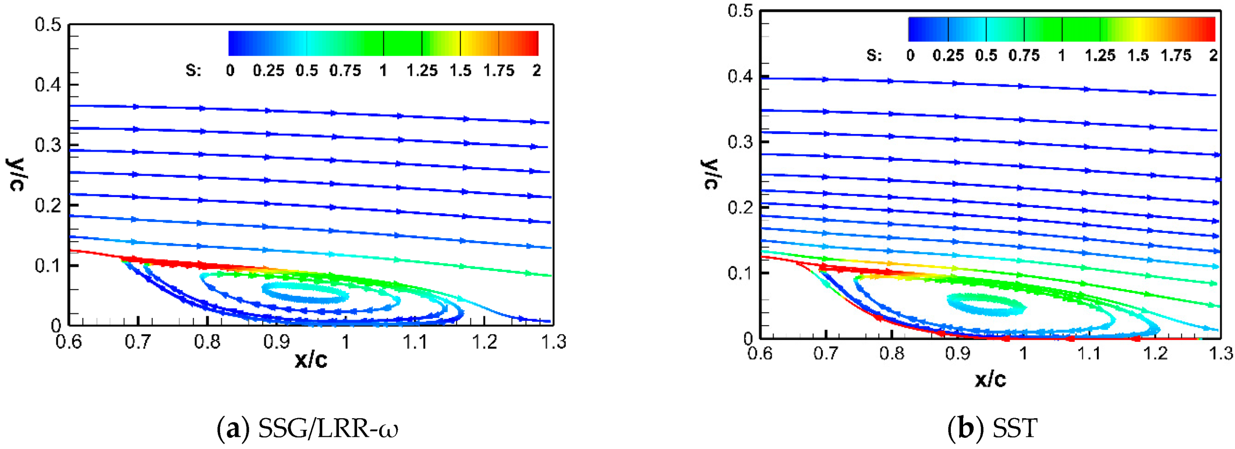
4.2. Lagging Reattachment

The main factor affecting the reattachment process is the shear between the upper edge of the separation bubble and the main flow. A stronger shear will create a stronger momentum exchange, giving the flow more energy to support earlier reattachment to the wall. In contrast, weaker shear will create a weaker momentum exchange and less shear stress, and so the reattachment will lag. For several typical positions in the shear layer above the separation bubble, the Reynolds shear stress calculated by the two models is compared in Figure 11. Clearly, the Reynolds shear stress in the shear layer predicted by the SST model is lower than the result predicted by SSG/LRR-ω, which means that the shear calculated by the SST model above the separation bubble is weaker and the reattachment point is located slightly downstream.

The Reynolds stress calculated by the SST model between the upper edge of the separation bubble and the mainstream is expressed as

$$-\overline{uv}=C_{\mu }\frac{k^2}{\epsilon }S={\nu }_{t}S.$$

(13)

Both the eddy–viscosity coefficient and the mean strain rate affect the prediction of Reynolds shear stress, so it is natural to extract the eddy–viscosity coefficient and the mean strain rate calculated by the two turbulence models to analyze their influence on the calculation of Reynolds shear stress. The eddy–viscosity coefficient and the average strain rate predicted by the two models at the upper edge of the separation bubble are plotted separately. Although the RSM does not contain the eddy–viscosity coefficient (as the Reynolds stress is solved directly), the eddy–viscosity coefficient itself is an artificially constructed physical quantity. Therefore, the Reynolds stress is divided by the average strain rate to obtain the corresponding “eddy–viscosity coefficient” in the SSG/LRR-ω model. In the hump example, the position between the top edge of the separation bubble and the mainstream is roughly between layers 160 and 172. Thus, the 160th, 164th, 168th, and 172nd layers of the grid are selected as representative locations to calculate the eddy–viscosity coefficient. In the NACA 4412 airfoil, the position of the shear layer above the separation bubble is roughly between layers 120 and 130. Thus, the 120th, 122nd, 125th, and 128th layers of the grids are selected as representative locations to calculate the eddy–viscosity coefficient. Furthermore, in the axisymmetric transonic bump, the shear layer between the top edge of the separation bubble and the mainstream is roughly located between grid layers 150 and 185. Thus, the 150th, 164th, 176th, and 184th grid layers are selected as representative locations to calculate the eddy–viscosity coefficient. The results are shown in Figure 12, Figure 13, Figure 14, Figure 15, Figure 16 and Figure 17.

In the hump and the NACA 4412 airfoil, ${\nu }_t$ and $S$ calculated by the SST model are lower than the values given by the SSG/LRR-ω model. In the axisymmetric transonic bump case, ${\nu }_t$ is still underestimated, while $S$ is slightly overestimated. Nevertheless, the Reynolds stress is still underestimated, indicating that the underestimation of ${\nu }_t$ has a more significant influence on the calculation of Reynolds stress. As mentioned above, the formula for calculating the eddy–viscosity coefficient in the shear layer above the separation bubble is:

$${\nu }_t=C_{\mu }\frac{k^2}{\epsilon }.$$

(14)

From Equation (14), it can be seen that ${\nu }_t$ is affected by Cμ, k, and ε. Among them, $C_{\mu }=0.09$, which is the square of ${\mathrm{a}}_1$ in Bradshaw’s relation. As mentioned in Section 4.1.2, although there is similar behavior to the thin shear layer outside the log layer, the value of ${\mathrm{a}}_1$ should be slightly smaller. That is, when calculating the eddy–viscosity coefficient between the upper edge of the separation bubble and the main flow, the value of $C_{\mu }$ (square of ${\mathrm{a}}_1$) is larger than in the actual situation. The turbulent kinetic energy predicted by the SSG/LRR-ω and SST models in the three cases is shown in Figure 18. The turbulent kinetic energy calculated by the SST model is smaller than that of the SSG/LRR-ω model.

Based on the above analysis, in the calculation of the SST model, the coefficient $C_{\mu }$ is relatively large, while the turbulent kinetic energy is underestimated compared with the SSG/LRR-ω model. Finally, ${\nu }_t$ is underestimated. It is hard to determine whether the dissipation rate $\epsilon$ is overestimated or underestimated. Let us examine the transport equation of $\epsilon$:

$$\frac{D\epsilon }{Dt}=P_{\epsilon 1}+P_{\epsilon 2}+P_{\epsilon 3}+P_{\epsilon 4}+T_{\epsilon }-D_{\epsilon }.$$

(15)

In this expression, $P_{\epsilon 3}$ is always very small, $P_{\epsilon 1}+P_{\epsilon 2}$ tends to 0 for y⁺ > 50, and $T_{\epsilon }$ is the transport term, which tends to 0 for y⁺ > 30. Thus, the main contribution term $P_{\epsilon 4}$ must balance the main consumption term $D_{\epsilon }$. Expanding these two items, we have:

$$P_{\epsilon 4}=-2\nu \left[\overline{\frac{\partial u_i}{\partial x_k}\frac{\partial u_i}{\partial x_m}\frac{\partial u_k}{\partial x_m}}\right].$$

(16)

$$D_{\epsilon }=2{\nu }^2\left[\overline{\frac{{\partial }^2{u}_i}{\partial x_k{x}_m}\frac{{\partial }^2{u}_i}{\partial x_k{x}_m}}\right].$$

(17)

These expressions are closely related to the third-order correlation term and the second-order derivative of the fluctuation velocity. However, the accuracy of the fluctuation velocity itself is relatively poor, which brings greater difficulties for the subsequent in-depth analysis. Further analysis is hampered by the fact that it is difficult to identify which of C_μ, k, and ε in ${\nu }_t$ is more influential or what the interaction among them is that causes ${\nu }_t$ to be underestimated. An additional complication is that ${\nu }_t$ itself has no obvious physical meaning and is only an artificially constructed coefficient.

The basis of the eddy viscosity model roots in the Boussinesq approximation, and the core of this assumption is to linearly correlate stress and strain with eddy viscosity coefficient. The Reynolds stress model obtains the Reynolds stress by directly solving the transport equation of the Reynolds stress. From this point of view, it has a more accurate and solid mathematical foundation than the eddy viscosity model when solving the Reynolds stress, so the value obtained should also more accurate. In the SSG/LRR-ω model, the so-called “eddy viscosity coefficient” obtained by dividing the Reynolds stress and strain can be used as a criterion for judging the eddy viscosity coefficient of the SST model. The lower value calculated by the SST model confirms the lower prediction accuracy caused by the approximation.

It can be concluded that the Boussinesq approximation followed by the EVM is a vital factor affecting the prediction accuracy. This reflects the obvious limitation of EVMs: the stress and strain are connected with linear assumptions, and the scalar ${\nu }_t$ is used to derive the isotropic Reynolds stress and express the effect of turbulence on the average flow field. In fact, turbulence is obviously anisotropic, and the relationship between stress and strain is much more complicated than the eddy–viscosity approximation. When the flow experiences extra rates of strain caused by rapid dilatation, out of plane straining, or significant streamline curvature, which give rise to unequal normal Reynolds stresses [24], the EVM based on the eddy–viscosity approximation does not perform well. These defects are obviously exposed under complicated conditions such as separated flow.

4.3. Difficulties of the Reynolds Stress Model

Although the results predicted by the RSM are slightly better than those of the two-equation model, there is still room for improvement. In simple shear flow, the Reynolds shear stress is expressed by:

$$\frac{D\overline{\mathit{uv}}}{Dt}=-\overline{v^2}\frac{\partial \overline{U}}{\partial y}+\overline{\frac{p}{\rho }\left(\frac{\partial u}{\partial y}+\frac{\partial v}{\partial x}\right)}-\frac{\partial }{\partial y}\left(\overline{u{v}^2}+\frac{\overline{pu}}{\rho }\right)+\frac{\mu }{\rho }\frac{{\partial }^2\overline{uv}}{\partial y^2}-2\frac{\mu }{\rho }\left\{\overline{\frac{\partial u}{\partial x}\frac{\partial v}{\partial x}}+\overline{\frac{\partial u}{\partial y}\frac{\partial v}{\partial y}}+\overline{\frac{\partial u}{\partial z}\frac{\partial v}{\partial z}}\right\}.$$

(18)

The last three terms,

$$\frac{\partial }{\partial y}\left(\overline{u{v}^2}+\frac{\overline{pu}}{\rho }\right)+\frac{\mu }{\rho }\frac{{\partial }^2\overline{uv}}{\partial y^2}-2\frac{\mu }{\rho }\left\{\overline{\frac{\partial u}{\partial x}\frac{\partial v}{\partial x}}+\overline{\frac{\partial u}{\partial y}\frac{\partial v}{\partial y}}+\overline{\frac{\partial u}{\partial z}\frac{\partial v}{\partial z}}\right\}.$$

are the diffusion and dissipation terms, and tend to be zero outside the laminar sublayer (y⁺ < 5). Only the production term and the pressure–strain term are balanced with each other. Therefore, the calculation of Reynolds shear stress has the most direct relationship with the modeling accuracy of the pressure–strain term. The significance of the Reynolds shear stress calculation and the effect of the pressure–strain term are discussed below. The transport equations of Reynolds normal stress in three directions in a simple shear flow are given by:

$$\frac{D\overline{u^2}}{Dt}=-2\overline{uv}\frac{\partial \overline{U}}{\partial y}+2\overline{\frac{p}{\rho }\frac{\partial u}{\partial x}}-\frac{\partial }{\partial y}\left(\overline{u^{2}v}\right)+2\frac{\mu }{\rho }\frac{{\partial }^2\overline{u^2}}{\partial y^2}-2\frac{\mu }{\rho }\left\{\overline{\frac{\partial u}{\partial x}\frac{\partial u}{\partial x}}+\overline{\frac{\partial u}{\partial y}\frac{\partial u}{\partial y}}+\overline{\frac{\partial u}{\partial z}\frac{\partial u}{\partial z}}\right\}.$$

(19)

$$\frac{D\overline{v^2}}{Dt}=0+2\overline{\frac{p}{\rho }\frac{\partial v}{\partial y}}-\frac{\partial }{\partial y}\left(\overline{v^3}+\frac{2\overline{pv}}{\rho }\right)+2\frac{\mu }{\rho }\frac{{\partial }^2\overline{v^2}}{\partial y^2}-2\frac{\mu }{\rho }\left\{\overline{\frac{\partial v}{\partial x}\frac{\partial v}{\partial x}}+\overline{\frac{\partial v}{\partial y}\frac{\partial v}{\partial y}}+\overline{\frac{\partial v}{\partial z}\frac{\partial v}{\partial z}}\right\}.$$

(20)

$$\frac{D\overline{w^2}}{Dt}=0+2\overline{\frac{p}{\rho }\frac{\partial w}{\partial z}}-\frac{\partial }{\partial y}\left(\overline{v{w}^2}\right)+2\frac{\mu }{\rho }\frac{{\partial }^2\overline{w^2}}{\partial y^2}-2\frac{\mu }{\rho }\left\{\overline{\frac{\partial w}{\partial x}\frac{\partial w}{\partial x}}+\overline{\frac{\partial w}{\partial y}\frac{\partial w}{\partial y}}+\overline{\frac{\partial \mathrm{w}}{\partial z}\frac{\partial w}{\partial z}}\right\}.$$

(21)

In the three-direction normal stress transport equations, only the stream-wise normal stress equation has a non-zero production term. Under the action of shear, the normal stress in the stream-wise direction will increase, while that in the other two directions will decrease when the flow is not affected by other external factors. After summing the three equations, the transport equation of turbulent kinetic energy can be derived, and the pressure–strain term is not included. The pressure–strain term does not affect the increase or decrease of turbulent kinetic energy but is redistributed in all three directions to promote the isotropic development of turbulence. When $\overline{u^2}$ is greater than $\overline{v^2}$ and $\overline{w^2}$, the excess stress will be supplemented to them through the redistribution of the pressure–strain term. Therefore, the intensity of $\overline{v^2}$ is guaranteed. As a critical physical property in the production term of $\overline{u^2}$, this means that $\overline{u^2}$ can continue to be generated, thereby forming a cycle and balance [20].

This redistribution mechanism is a necessary factor for the maintenance of 3D turbulence. However, the isotropic state can only be reached after a very long time and the production term disappears. There are two critical points here. One is that it is vital to predict the anisotropy of normal stresses correctly in turbulence calculations. The other is that, without this redistribution mechanism, shear stress cannot be generated [20]. Although the redistribution effect of the pressure–strain term plays a decisive role in the production of Reynolds shear stress, the modeling of the pressure–strain term is almost the most challenging step in the construction of the RSM. The reason is that accurate experimental data cannot be measured for verification of the modeling process. Therefore, the modeling of this term requires excellent creativity.

In the calculation examples in this article, although the SSG/LRR-ω model is slightly more accurate than the SST model in the prediction of the separation onset and the reattachment point, this does not mean that the calculation accuracy of the SSG/LRR-ω model is superior to that of the SST model in all cases. Compared with the SST model, the SSG/LRR-ω model has a shorter development time and has not undergone many tests, so sometimes the SST model performs better. For example, when the NACA4412 airfoil trailing edge is separated, the SST model gives a more realistic separation bubble structure in Figure 6 and we can see Figure 2 where the SST over-predicts the reattachment point somewhat more, but gives a better profile of Cf than the SSG/LRR near the reattachment. This shows that there are still some defects in the modeling process of the Reynolds stress transport equation, which need to be further analyzed and corrected by researchers, so as to develop a more perfect model.

5. Conclusions

In this study, the SSG/LRR-ω and SST models were selected as representatives of RSMs and two-equation models, and the turbulent separation problem was analyzed to identify the reasons for advanced separation and lagging reattachment that may occur during the calculation. Based on the underestimation of shear stress, the underlying mechanism of the performance differences of the models was further analyzed in terms of equation construction, basic assumptions, and modeling idea.

• The SST model underestimates the Reynolds stress upstream of the separation onset in the actual flows, leading to advanced separation. This phenomenon occurs because the SST model imposes $P_k=\epsilon$ [20] as a result of Menter’s modification of the eddy–viscosity coefficient by introducing Bradshaw’s relation ($-\overline{uv}=\rho a_{1}k$). However, this condition is strictly valid only in the log layer. When it is extrapolated to other areas or encounters a large adverse pressure gradient in the separated flow, the equilibrium condition $P_k=\epsilon$ cannot be satisfied, and the coefficient $a_1$ in Bradshaw’s relation needs to be corrected. Although the SST model noticeably enhances the prediction of the separated flows using Menter’s modified eddy–viscosity coefficient, the relation is too harsh, causing the phenomenon of separation to occur in advance.
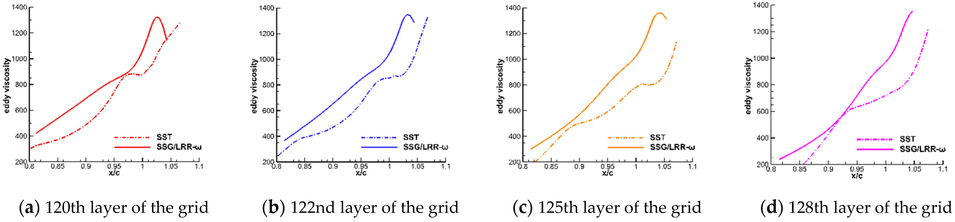
• The SST model underestimates the Reynolds stress in the developing shear layer above the separation bubble, resulting in reattachment too far downstream. The reason for this phenomenon is different from that of the advanced separation. The modeling error of the eddy–viscosity coefficient and the calculation error of the average strain rate both introduce losses to the calculation accuracy of Reynolds stress. According to our analysis, the main effect on the Reynolds stress is caused by the underestimation of the eddy–viscosity coefficient, with relatively little effect caused by the average strain rate. In addition, the eddy–viscosity coefficient contains turbulent kinetic energy and dissipation. These components affect and restrict each other. Thus, the specific mechanism is very complex.
• The SSG/LRR-ω model obtains the Reynolds stress directly by solving the Reynolds stress transport equation. Most of the errors come from the modeling of the closure term, especially the modeling of the pressure–strain term. The inability to obtain accurate experimental data limits the accuracy with which the pressure–strain term can be modeled, but the redistribution of the pressure–strain term plays a decisive role in the production of Reynolds shear stress.

In summary, the eddy–viscosity approximation is highly important in the prediction accuracy of the SST model. Due to the solid mathematical and physical foundation of the SSG/LRR-ω model, it retains more flow field information when solving for the Reynolds stress. By contrast, the SST model may lack accuracy in certain properties (e.g., the Reynolds stress) that are important for flow prediction after using the eddy–viscosity approximation, which is a relatively crude simplification. This has a considerable impact on the prediction accuracy of turbulent flows.

The above conclusions explain why the SST and SSG/LRR-ω models tend to mismatch the separation onset and reattachment points in separated flows. Moreover, the problems at the theoretical level pointed out by Leschziner et al. [20] correspond to the performance in actual flows, which improves our overall knowledge of this issue. The results of this study provide some reference and guidance for better application of turbulence models in practical engineering projects and further examination of flow mechanisms in scientific research, which we hope will lead to the development of more general and accurate turbulence models.

References

1. Chen, M.Z. Fundamentals of Viscous Fluid Dynamics; Higher Education Press: Beijing, China, 2004. [Google Scholar]
2. Pla, B.; Jp, B. On the modelling turbulent transition in turbine cascades with flow separation. Comput. Fluids 2019, 181, 160–172. [Google Scholar]
3. Yan, C.; Qu, F.; Zhao, Y.T.; Yu, J.; Wu, C.H.; Zhang, S.H. Review of development and challenges for physical modeling and numerical scheme of CFD in aeronautics and astronautics. Acta Aerodyn. Sin. 2020, 38, 829–857. [Google Scholar]
4. Slotnick, J.; Khodadoust, A.; Alonso, J.; Darmofal, D.; Gropp, W.; Lurie, E.; Mavriplis, D. CFD Vision 2030 Study: A Path to Revolutionary Computational Aerosciences, Mchenry County Natural Hazards Mitigation Plan; NASA: Hampton, VA, USA, 2014. [Google Scholar]
5. Driver, D.M.; Seegmiller, H.L. Features of a reattaching turbulent shear layer in divergent channel flow. AIAA J. 1984, 23, 163–171. [Google Scholar] [CrossRef]
6. Zhao, R.; Yan, C. Evaluation of engineering turbulence models for complex supersonic flows. J. Beijing Univ. Aeronaut. Astronaut. 2011, 37, 202–205+215. [Google Scholar]
7. Eisfeld, B.; Rumsey, C.; Togiti, V. Verification and Validation of a Second-Moment-Closure Model. AIAA J. 2016, 54, 1524–1541. [Google Scholar] [CrossRef]
8. Bush, R.H.; Chyczewski, T.S.; Duraisamy, K.; Eisfeld, B.; Rumsey, C.L.; Smith, B.R. Recommendations for Future Efforts in RANS Modeling and Simulation. In Proceedings of the AIAA Scitech 2019 Forum, San Diego, CA, USA, 7–11 January 2019. [Google Scholar]
9. Rumsey, C.L. Application of Reynolds Stress Models to Separated Aerodynamic Flows. In Differential Reynolds Stress Modeling for Separating Flows in Industrial Aerodynamics; Springer: Berlin/Heidelberg, Germany, 2015. [Google Scholar]
10. Menter, F.R. Zonal Two Equation k-w Turbulence Models for Aerodynamic Flows. In Proceedings of the 23rd Fluid Dynamics, Plasmadynamics, and Lasers Conference, Orlando, FL, USA, 6–9 July 1993. [Google Scholar]
11. Rodriguez, S. Applied Computational Fluid Dynamics and Turbulence Modeling: Practical Tools, Tips and Techniques; Springer: Berlin/Heidelberg, Germany, 2019. [Google Scholar]
12. Raje, P.; Sinha, K. Anisotropic SST turbulence model for shock-boundary layer interaction. Comput. Fluids 2021, 228, 105072. [Google Scholar] [CrossRef]
13. Menter, F.R.; Kuntz, M.; Langtry, R. Ten years of industrial experience with the SST turbulence model. Turbul. Heat Mass Transf. 2003, 4, 625–632. [Google Scholar]
14. Eisfeld, B.; Brodersen, O. Advanced Turbulence Modelling and Stress Analysis for the DLR-F6 Configuration. In Proceedings of the 23rd AIAA Applied Aerodynamics Conference, Toronto, ON, Canada, 6–9 June 2005. [Google Scholar]
15. Rumsey, C.L. Turbulence Modeling Resource. Available online: http://turbmodels.larc.nasa.gov (accessed on 13 November 2021).
16. Rumsey, C.L. Turbulence Modeling Verification and Validation (Invited). In Proceedings of the 52nd Aerospace Sciences Meeting, National Harbor, MD, USA, 13–17 January 2014. [Google Scholar]
17. Krist, S.L.; Biedron, R.T.; Rumsey, C.L. CFL3D User’s Manual; (Version 5.0); NASA Langley Technical Report Server: Hampton, VA, USA, 1998. [Google Scholar]
18. Greenblatt, D.; Paschal, K.B.; Yao, C.S.; Harris, J.; Schaeffler, N.W.; Washburn, A.E. Experimental Investigation of Separation Control Part 1: Baseline and Steady Suction. AIAA J. 2006, 44, 2820–2830. [Google Scholar] [CrossRef]
19. Alber, I.E.; Bacon, J.W.; Masson, B.S.; Collins, D.J. An Experimental Investigation of Turbulent Transonic Viscous-Inviscid Interactions. AIAA J. 2015, 11, 620–627. [Google Scholar] [CrossRef]
20. Leschziner, M. Statistical Turbulence Modelling for Fluid Dynamics-Demystified: An Introductory Text for Graduate Engineering Students; Imperial College Press: London, UK, 2015. [Google Scholar]
21. Zhu, K.Q.; Xu, C.X. Viscous Fluid Mechanics; Higher Education Press: Beijing, China, 2009. [Google Scholar]
22. Bertelrud, A.; Nordstrom, J. Experimental and computational investigation of the flow in the leading edge region of a swept wing. In Proceedings of the AIAA 16th Fluid and Plasmadynamics Conference, Danvers, MA, USA, 12–14 July 1983. [Google Scholar]
23. Liou, W.W.; Huang, G.; Shih, T.H. Turbulence model assessment for shock wave/turbulent boundary-layer interaction in transonic and supersonic flows. Comput. Fluids 2000, 29, 275–299. [Google Scholar] [CrossRef]
24. Wilcox, D.C. Turbulence Modeling for CFD; DCW Industries: La Cañada Flintridge, CA, USA, 2006. [Google Scholar]
Figure 1. 2D NASA wall-mounted hump separated flow; sketch of the geometry and boundary conditions.
Aerospace 09 00020 g001
Figure 2. Skin-friction distribution of the hump.
Aerospace 09 00020 g002
Figure 3. Streamlines near the hump: (a) the result of the SSG/LRR-ω model; (b) the result of the SST model.
Aerospace 09 00020 g003
Figure 4. Subsonic flow around NACA 4412 airfoil; boundary conditions [15].
Aerospace 09 00020 g004
Figure 5. Skin-friction distribution of the NACA 4412 airfoil.
Aerospace 09 00020 g005
Figure 6. Streamlines of the NACA 4412 airfoil: (a) the result of the SSG/LRR-ω model; (b) the result of the SST model.
Aerospace 09 00020 g006
Figure 7. Axisymmetric transonic bump; grid structure and boundary conditions [15].
Aerospace 09 00020 g007
Figure 8. Axisymmetric transonic bump; skin-friction distribution.
Aerospace 09 00020 g008
Figure 9. Streamlines near the bump: (a) the result of the SSG/LRR-ω model; (b) the result of the SST model.
Aerospace 09 00020 g009
Figure 10. Comparisons of Reynolds shear stress profiles of the hump.
Aerospace 09 00020 g010
Figure 11. Profiles of Reynolds shear stress: (a) the result of the SSG/LRR-ω model; (b) the result of the SST model.
Aerospace 09 00020 g011
Figure 12. Profiles of the eddy–viscosity coefficient of the hump.
Aerospace 09 00020 g012
Figure 13. Streamline diagram colored according to average strain rate of the hump.
Aerospace 09 00020 g013
Figure 14. Profiles of the eddy–viscosity coefficient of the NACA 4412 airfoil.
Aerospace 09 00020 g014
Figure 15. Streamline diagram colored according to the average strain rate of the NACA 4412 airfoil.
Aerospace 09 00020 g015
Figure 16. Profiles of the eddy–viscosity coefficient of the axisymmetric transonic bump.
Aerospace 09 00020 g016
Figure 17. Streamline diagram colored according to the average strain rate of the axisymmetric transonic bump.
Aerospace 09 00020 g017
Figure 18. Turbulent kinetic energy profiles.
Aerospace 09 00020 g018