Data-Driven Transition Models for Aeronautical Flows with a High-Order Numerical Method

Abstract

Over the past years, there has been innovative ideas about data-driven turbulence modeling proposed by scholars all over the world. This paper is a continuity of these significant efforts, with the aim of offering a better representation for turbulence physics. Previous works mainly focus on turbulence viscosity or Reynolds stress, while there are few works for turbulence transition. In our work, two mapping functions between average flow parameters and transition intermittency, a virtual physical quantity describing the amount of turbulence at a given position, are refactored, respectively, with neuron networks and random forests. These two functions are then coupled with the Spalart–Allmaras (SA) model to reconstitute two models for transition prediction. To demonstrate that these two coupled models provide improved prediction accuracy on transition compared with previous SA models, we conduct test cases all under a high-order weighted compact nonlinear scheme (WCNS). The prediction results of both coupled models significantly improved the capture of natural transitions occurring in the flows. Furthermore, the interpolation generalisation and extrapolation generalisation abilities of the coupled models are also demonstrated in this paper. The results emphasize the potential for machine learning as a supplementary in turbulence transition modeling.

1. Introduction

Predicting a transition from laminar flow to turbulent flow accurately is of significant importance for mechanical-engineering calculations and turbulent physics, as transition has a huge effect on drag, aero-heating, flight efficiency and energy consumption. Despite the boom in computer hardware and high-performance computing, high-fidelity simulations, such as direct numerical simulation (DNS) and large-eddy simulation (LES), have not been applied feasibly to complex industrial flows [1] for the exponential growth (proportionate to $R{e}^{\frac{9}{4}}$) of computational cost with the increase in Reynolds number. As a result, Reynolds-averaged Navier–Stokes (RANS) models, where empirical closures are used to model Reynolds stress, still dominates engineering applications of turbulent flows owing to their high efficiency [2,3]. Quite a lot of well-developed RANS-based methods, such as the SA model [4,5] and SST [6,7] model, are widely used in numerical simulations of industrial flows. However, traditional RANS models do not have the ability to predict boundary layer transition well itself, so improvements are needed for engineering calculation.

The correlation-based transition model, which was first proposed by Dhawan and Narasimha [8], is one of the most acceptable RANS-based transition models at present because of its high computation efficiency. It uses intermittency, $\gamma$, to represent the time-dependent amount of turbulence in a flow at a fixed location. This uses the function $I(x,y,z,t)$ to describe the phenomenon of intermittence and defines the function value as 0 in laminar while 1 in turbulence. Intermittency $\gamma$, needing extra transport equations to obtain, can be defined as the time average of the function.

$$\gamma (x,y,z,t)=\frac{1}{T}{\int }_0^{T}I(x,y,z,t)dt$$

(1)

Dhawan and Narasimha [8] proposed an algebraic intermittency form with the method of fitting. Similarly, Klebanoff et al. [9] postulated another empirical formula aimed at solving flat plate turbulence problems. However, the results of these two models in complex flows are not that reliable as vortex structures are not considered in such empirical solutions. Libby [10] first applied intermittency-involved transport equation to perform computations on turbulence, and Dopazo [11] worked on the perfection of this idea. Then, it was followed by research focused on improving predictions based on an intermittency model for the number of flows. Among them, the model presented by Cho and Chung [12] is most representative, and can simulate the $\gamma$ distribution of planar jet, circular jet, planar mixed layer and wake. Steerlant and Dick [13] put forward a transport equation for $\gamma$, but the results of it are not that good in a normal direction. Huang and Suzen [14] construct a $\gamma$ function combining the two models mentioned above. These models, however, cannot be used in parallel computing as a single boundary layer cannot be calculated with different kernel processors. Moreover, momentum-thickness $\theta$ is hard to obtain when using non-structural meshes. To solve these problems, Menter et al. [15,16] replaced Re based on momentum-thickness by $R{e}_{\theta }$ based on local strain rate, and developed the four-equation transitional SST model, which can also be called the SST-$\gamma$-$R{e}_{\theta }$ model. The conservative four-equation SST transition model based on non-dimensional $\gamma$ and $Re$ can be written as:

$$\frac{\partial \left(\rho \gamma \right)}{\partial t}+\frac{\partial \left(\rho \gamma u_j\right)}{\partial x_j}=\frac{1}{Re}\frac{\partial }{\partial x_j}\left[(\mu +{\sigma }_{\gamma }{\mu }_t)\frac{\partial \gamma }{\partial x_j}\right]+P_{\gamma }-E_{\gamma }$$

(2)

$$\frac{\partial \left(\rho {\widetilde{Re}}_{\theta t}\right)}{\partial t}+\frac{\partial \left(\rho {\widetilde{Re}}_{\theta t}{u}_j\right)}{\partial x_j}=\frac{1}{Re}\frac{\partial }{\partial x_j}\left[{\sigma }_{\theta t}(\mu +{\mu }_t)\frac{\partial {\widetilde{Re}}_{\theta t}}{\partial x_j}\right]+P_{\theta t}$$

(3)

It has been verified that this model is able to predict the developments of different kinds of transitions, natural transition, separation transition and bypass transition included [15,17,18]. However, these models rely on empirical correlations to a great extent. For different conditions, different calibration works on these empirical correlation equations are needed, which influences the generalization ability of the model. As a result, a $\gamma$-based model independent from empirical correlations with low computational costs is of urgent need.

In recent years, the rapid development of machine-learning methods has provided industrial simulations a totally new way. Research on data-driven methods that augment engineering calculation are emerging, such as the work of Chia et al. [19,20]. Using a machine-learning method to find out the inner relationship between the transition and local average quantities has the potential to improve the efficiency and reliability of transition predictions. Some researchers apply machine-learning methods to improve or replace existing turbulence models. Singh et al. [21] postulate a data-driven paradigm for turbulence model augmentation and use inverse modeling to extract the spatial distribution of discrepancies, which provides improved prediction accuracy for flow separation. Duraisamy and Zhang et al. [22] reconstruct $\gamma$-transport equation using neural networks and Gaussian progress (GP), leading to a more exact result of the transition to a series of T3 flat plate. Zafar et al. [23] use a recurrent neural network to calculate N-factor envelope and the transition. These studies show that it is possible to use machine learning to build transition models. However, the generalization ability of these models for other geometric profiles or initial flow conditions still needs further research. There are also many studies focusing on replacing traditional models with machine-learning closure, to make up for the inherent defect of RANS models. Ling et al. [24] use a tensor basis neural network (TBNN) to build a Reynolds stress anisotropy tensor model from high-fidelity simulation data. They find that only input features ensuring Galilean invariance can guarantee the rotational invariance in predicted eigenvalues. Their results show a nice prediction on both corner vortices in duct-flow cases and flow separations in wavy-wall cases. Despite their work representing a significant step towards improving RANS prediction accuracy, the astringency of this tightly coupled system remains to be verified. In this article, we introduce data-driven algorithms into the present home-made weighted-compacted-nonlinear-scheme (WCNS) CFD solver to represent the primary hypothesis of SA equations and demonstrate its prediction and generalization ability. Deng et al. [25] constructed a CNS scheme and, to improve the efficiency and accuracy of the calculation, Deng et al. [26] introduced a weighted-compact into CNS and constructed a high-order WCNS scheme. Nonomura [27,28] generalized the WCNS scheme to an arbitrary order and verified that the scheme has better free-flow preservation performance and robustness than the WENO scheme. The superiority of the high-order WCNS scheme on high resolution, heat-flux capture, surface pressure and drag distribution has been verified in extensive flow situations [29,30,31]. The core idea of our work is that machine-learning methods can effectively create a descriptive universal model for transition processes by taking advantage of data from high-order convergent flow fields.

This paper is organized as follows. In Section 2, the numerical methods, including the SST-$\gamma$-$R{e}_{\theta }$ transition methods and SA turbulence model are briefly introduced. Furthermore, Section 2 will describe the construction process of an intermittency-involved model coupled with machine-learning methods. In Section 3, the generalization ability of the tightly coupled transition-predictive system with both NN and RF machine-learning methods is verified using several cases. In Section 4, the conclusions and future works are given.

2. Methodology

An SA model is effective and robust at computing turbulent flows. There has been explorations into combining a $\gamma$-$R{e}_{\theta }$ model with an SA model, with the purpose of improving the efficiency of calculations. Nevertheless, turbulent kinetic energy k and its dissipation rate $\omega$ at some locations of the flow field, which SA models do not give values to, are needed in hypothetical-SA-$\gamma$-$R{e}_{\theta }$ transition models. As a result of this, this combination calls for new closure models. Here, machine-learning methods are used for this closure.

The construction of the model can be divided into two processes, respectively, the data-learning process and coupling-solution process. During the process of data learning, a sandbox function is made up using a machine-learning method. Next, when conducting the coupling solution, the model confirmed before is embedded within a CFD solver. Per one or some iterations of the CFD solver, local average quantities $q(q_1,q_2,\dots ,q_n)$ will be introduced into the confirmed model to obtain the intermittency distribution of the whole flow field, and, finally, the distribution will be introduced back to the CFD solver. The main framework of the coupled solution is depicted in Figure 1. The construction process of both viscosity models and machine-learning models will be discussed below.

2.1. Turbulence Model

2.1.1. SA Turbulence Model

The SA turbulence model is one of the one-equation RANS models depicting the transport of specific turbulent viscosity, $\tilde{\nu }$. The governing equation of SA model is:

$$\frac{D\tilde{\nu }}{Dt}=P_{\nu }-D_{\nu }+\frac{1}{\sigma }[▽\times ((\nu +\tilde{\nu })▽\tilde{\nu })+C_{b2}{(▽\tilde{v})}^2]$$

(4)

where $\nu$ is turbulent kinematic viscosity. The model constructs Reynolds-stress tensor ${\tau }_{i,j}$ by using Boussinesq approximation and computations on turbulent eddy viscosity ${\nu }_t$.

$${\nu }_t=\tilde{\nu }{f}_{v1},$$

(5)

$$f_{v1}=\frac{{\chi }^3}{{\chi }^3+C_{v1}^3},$$

(6)

$$\chi =\frac{\tilde{\nu }}{\nu }$$

(7)

The production and destruction of $\tilde{\nu }$ is defined using the wall distance d as:

$$P_{\nu }=C_{b1}\widehat{S}\tilde{\nu }$$

(8)

$$D_{\nu }=C_{w1}{f}_w{\left(\frac{\tilde{\nu }}{d}\right)}^2$$

(9)

where

$$\widehat{S}=\Omega +\frac{\tilde{\nu }}{{\kappa }^2{d}^2}{f}_{\nu 2},f_{\nu 2}=1-\frac{\chi }{1+\chi f_{\nu 1}}$$

(10)

$$f_w=g{\left(\frac{1+C_{w3}^6}{g^6+C_{w3}^6}\right)}^{\frac{1}{6}},g=r+C_{w2}(r^6-r)$$

(11)

$$r=min(\frac{\tilde{\nu }}{\widehat{S}{\kappa }^2{d}^2},10)$$

(12)

The constants mentioned above value as:

$$C_{b1}=0.1355,C_{b2}=0.622,\sigma =\frac{2}{3},\kappa =0.41$$

(13)

$$C_{w2}=0.3,C_{w3}=2,C_{\nu 1}=7.1,C_{t3}=1.2$$

(14)

$$C_{t4}=0.5,C_{w1}=\frac{C_{b1}}{{\kappa }^2}+\frac{1+C_{b2}}{\sigma }$$

(15)

Figure 1. Main framework of coupling solution.

Figure 1. Main framework of coupling solution.

Referring to correlation-based transition models, they use intermittency to control the production of turbulence before and during transition process; thus, amending the full turbulence hypothesis is practical. Intermittency $\gamma$ describes the amount of turbulence at a fixed position in the flow objectively. Use of machine learning makes it possinle to find out the inner relationship between local average and $\gamma$. Combining $\gamma$ into the SA model, the repressed production and destruction terms can be defined as:

$${\tilde{P}}_{\nu }={\gamma }_{pre}\times P_{\nu }$$

(16)

$${\tilde{D}}_{\nu }=min[max({\gamma }_{pre},\beta ),1.0]\times D_{\nu },\beta =0.3$$

(17)

where $\beta$ is the correction factor of the destruction term.

As the SA model takes no account for the far-field value of turbulent eddy viscosity ${\nu }_t$, Medida et al. [32] assume the ${\nu }_t$ constant in the whole flow field when coupling the $\gamma$-$R{e}_{\theta }$ model with the SA model. The turbulent eddy viscosity ${\nu }_t$ of a free flow is also assumed as a constant in our work and is used as one of the input features in the machine-learning process.

2.1.2. Parameter Calibration

The values of the correction factor of the destruction term $\beta$ and far-field variety ${\nu }_{t\infty }$ have to change, respectively, to ensure the compatibility of the SA model after the modification above. For a whole new geometric profile or flow condition, a workout machine-learning algorithm can calculate, respectively, $\gamma$ needed directly with other local average quantities without any other transition model.

T3A flat transition plate case is used here for data calibration. The mesh is shown in Figure 2, which has 325 cells in x-direction and 108 cells in y-direction. Mesh adjacent to the wall or at the leading edge of the plate has been refined. As the results show in Figure 3, a ${\nu }_{t\infty }$ value too large will lead to a predicted transition position much earlier than that of the physical truth; thus, ${\nu }_{t\infty }$ for calibration was ultimately set as $1.0\times {10}^{-8}$. To control the friction coefficient of a turbulent area, the correction factor of the destruction term $\beta$ was set as 1.0.

2.1.3. Mesh-Dependency Study

A mesh-dependency study, as well as credibility analysis, is crucial before an ML prediction model is built. Here, verification for the coupled CFD solution is given. It is worth noting that the performance of a whole machine learning significantly depends on the training data and other specific machine-learning methods and hyper-parameters; thus, here we assume the $\gamma$ distribution predicted by the machine-learning model to be the same as that of the training data calculated by the $\gamma$-$R{e}_{\theta }$ model.

A still transition plate case is used for the mesh-dependency study. Three sets of T3A plate meshes are used here, specifically, $216\times 72$, $324\times 108$, and $486\times 162$ (flow direction × normal direction) as coarse mesh, medium mesh and fine mesh. The mesh number of the coarse mesh is 2/3 of that of the medium mesh in both directions, while the mesh number of the medium mesh is 2/3 of the fine mesh on both directions. Figure 4 shows the results calculated by machine-learning-coupled CFD, respectively, based on a second order MUSCL scheme and five order WCNS scheme of different sets of meshes. The $C_f$ of different sets of meshes is in better accordance with each other than that of MUSCL scheme, and agrees with the experiments well. This implies that the high-order WCNS scheme has lower numerical diffusion, thus, better dependency. In addition, the credibility of the machine-learning-coupled CFD frame is verified.

2.2. Machine-Learning Method

A data-driven method is used to obtain the mapping relationship between local average flow quantities and intermittency distribution to replace labor empirical functions. This is a kind of regression question. Therefore, we use a supervised machine-learning method, in which marked data is used for training, and numerical predictions are given. Neural networks and random forests are two of the most popular method to solve regression questions. The basic theory on these two methods is introduced in chief below.

2.2.1. Random Forests

Random forests is an algorithm integrated by decision trees, a kind of easily supervised learning algorithm used in classification or regression problems. A decision tree has a tree structure generally consisting of a root node and some tree nodes. Tree nodes can be divided into internal nodes, used for attribute tests and the division of new tree nodes, and leaf nodes, a representation of the outcome of the decision. As is shown in Figure 5, a single decision tree follows the conception of “divide-and-rule”. Beginning with a root node, all samples collected go through attribute tests for every internal node, and, finally, are divided into several classes.

During the generation process of a decision tree, the key step is to choose an optimal trait for each node. The Gini Index is often used in trait choosing. Generally speaking, the data sets represented by branches are expected to be more similar to the details of the tree structure. The impurity level of data set S can be measured by impurity level function $H\left(x\right)$. For regression questions, $H\left(S\right)$ can be calculated as:

$$H\left(S\right)=\frac{1}{N}\sum _{i=1}^N{(y_i-\overline{y})}^2$$

(18)

where N is the number of samples, and $\overline{y}$ is the average of the targets available. Therefore, the Gini Index of attribute x can be calculated with $H\left(S\right)$ as:

$$GiniIndex(S,x)=\sum _{m=1}^M\frac{|S^m|}{\left|S\right|}H\left(S^m\right)$$

(19)

where M is the number of values available for attribute x and $S^m$ is the sample set of x in data set S whose value is $x^m$. Therefore, under all these assumptions, optimal attribution a can be expressed as:

$$a=argminGiniIndex(S,x)$$

(20)

Essentially, random forest is adopted with the Bagging ensemble-learning method, which creates decision trees for the purpose of obtaining a better model for generalization. Using put-and-return samples, the method is able to generalize several different data sets with only one data set. Based on these data sets, different decision trees can be trained to support the learning process. Moreover, a randomness method is introduced to the algorithm. In contrast to other decision tree models, a random forests model does not need to calculate the Gini Index of each attribute as it chooses several attributes randomly and selects the best from them, so the diversity of different decision trees guaranteed as optimal attributes differs every time. Due to the randomness of the attributions, models trained in random forests are armed with better generalization ability.

2.2.2. Neural Networks

Neural network is another kind of classical machine-learning algorithm. A neural network, as depicted in Figure 6, connects layers of neurons with each other to form a network, including some hidden layers and one output layer.

A neuron is a basic computation unit that takes a weighted sum of its inputs (which are the outputs of its up layer), and sends that weighted sum through an activation function. More specifically, an input layer consists of a set of local averages $q=(q_1,q_2,\dots ,q_n)$ representing different attributions of the flow field. These inputs go through weighted connections and get to the next hidden layer, are compared with the threshold of the layer, and are transformed by non-linear activation functions. Having gone through a hidden layer, the feature information is transformed to a new feather space until the final results are output. For regression predictions, there is no need to add non-linear functions to the output layer, and the result is directly a linear combination of weight eigenvectors. For the network depicted in Figure 6, the jth component of the first layer $z_j^{\left(1\right)}$ is computed as follows:

$$z_j^{\left(1\right)}={\varphi }^{\left(1\right)}(\sum _{i=1}^3{w}_{ij}^{\left(1\right)}{q}_i-c_i^{\left(1\right)})$$

(21)

where $\varphi$ is the non-linear activation function; $w_{ij}$ is the weight between this layer and its up layer; and $c_{ij}$ is the threshold at this neuron node. Finally, the result of the output layer is computed as:

$$f\left(\mathit{q}\right)={\varphi }^{\left(3\right)}(\sum _{i=1}^m{w}_{ij}^{\left(3\right)}{z}_i^{\left(2\right)}-c_j^{\left(3\right)})$$

(22)

For a fixed network structure, the prediction ability of the neuron network algorithm depends directly on the value of weights and bias term of each layer. The process of confirming the set of optimal values of the parameters is called training or learning process of the network. Once a training set is ensured, the parameters of each node can be optimized using a back propagation algorithm. For example, for training sample $(x,y)$, the optimization process is:

$$\begin{array}{c}\hfill w_i\leftarrow w_i+\mathsf{\Delta }{w}_i\\ \hfill \mathsf{\Delta }{w}_i=\eta (y-\widehat{y})x_i\end{array}$$

(23)

where $\widehat{y}$ is the output of the network; and $\eta \in (0,1)$ is the learning rate.

2.3. Data-Driven Transition Model

2.3.1. Data Sets

Intermittency $\gamma$ is chosen to be predicted by machine learning. Compared with predicting Reynolds stress tensor or the turbulent viscosity directly, the prediction of $\gamma$ can exclude the influence of extreme outliers and nonphysical solutions, making the model more robust and smooth. However, on the other hand, we cannot obtain the real distribution of $\gamma$, a physical quantity does not exist in the real flow field, from high-fidelity data such as DNS or LES directly. Even a set of intermittencies can be calculated by high-fidelity data by Bayesian inversion; the result-oriented method cannot help with finding a single confirmed solution. The $\gamma$ field could not represent with the real flow field conditions, even though considerable computational resources are consumed. Furthermore, the performance of a machine-learning method is sensitive to training data, inner machine-learning parameters (so-called hyper-parameters), the loss functions used, and so on. Therefore, this research does not focus on how precise an extreme model performs, but explores the generalization ability of the application of a machine-learning method to transition models.

After overall consideration of the reasons above, intermittency $\gamma$ calculated with an SST-$\gamma$-$R{e}_{\theta }$ model under WCNS is chosen to be as the “truth value”, while results calculated by a modified SA model is chosen to be the input data set.

The key point of improving the prediction ability of an SA model by inserting a machine-learning algorithm is whether the model can make out a predictive $\gamma$ field accurate enough when given a completely new geometric configuration or free flow condition, so choosing training traits that can represent the transition process is another crucial problem. In transition problems, there exists complicated non-linear mapping relationships between the intermittency state of some points and the local averages, whose numerical functions are hard to obtain. Related works of Bas et al. [33] constructed a numerical model with two local variables to predict where the transition begins. Their model is not adaptable to some conditions, while their results are sufficient to indicate that it matters in turbulence prediction to construct proper local variables. Ling et al. [25] has verified that input variables are supposed to meet Galilean rotation invariance to make final results meet Galilean rotation invariance in corresponding coordinates. To meet this condition, ten local variables meeting Galilean rotation invariance are chosen to be input features of our machine-learning model, as

Table 1. Input features.

Feature	Sign
Density	$\rho$
Turbulence intensity	$Tu$
Nearest wall distance	$d_w$
Ratio of modified viscosity  to kinematic viscosity	$\frac{\tilde{\nu }}{nu}$
Scalar function 1	$Tr\left(S^2\right)$
Scalar function 2	$Tr\left({\mathsf{\Omega }}^2\right)$
Scalar function 3	$Tr\left({\mathsf{\Omega }}^{2}S\right)$
Normalized strain rate	$\left|\right|S\left|\right|/\left(\right|\left|S\right||+|\left|\mathsf{\Omega }\right|\left|\right)$
Q criterion	$\frac{\frac{1}{2}{\left(\right|\left|\mathsf{\Omega }\right||}^2-{\left|\right|S\left|\right|}^2)}{\frac{1}{2}{\left(\right|\left|\mathsf{\Omega }\right||}^2-{\left|\right|S\left|\right|}^2{)+|\left|S\right||}^2}$
Vortex Reynolds number (strain rate)	$\frac{\rho d_w^{2}S}{\mu }$

depicts. These input features have to use local non-dimensional variables to ensure the generalization ability of the model. They consist of free flow conditions, local averages and its derivations. In neuron networks, local features are the entrances to the input layer, while in random forests, these features act as the decisive attributes of the nodes.

2.3.2. Activation Function and Loss Function

In a neuron network algorithm, weighted correlations can only achieve linear fitting, so non-linear activation functions are needed for non-linear descriptions. Here, an ReLU function is chosen considering the characteristic of $\gamma$. It is defined as:

$$ReLU\left(x\right)=max(0,x)$$

(24)

An activation function can not only introduce non-linear conversion into a neuron network, but can also make it continuously differentiable so that it can be used in optimization algorithms such as gradient descent. The curve of ReLU function is depicted in Figure 7.

Another important indicator for machine-learning models is loss function. Here it is set as:

$$Loss=\frac{1}{N}\sum _{k=1}^N{({\overline{\gamma }}_{\kappa }-{\gamma }_{\kappa }\left(q_i\right))}^2$$

(25)

where ${\overline{\gamma }}_{\kappa }$ expresses the true value of the test data, ${\gamma }_{\kappa }\left(q_i\right)$ is the output of the machine-learning method, and N is the total number of the training data.

2.3.3. Parameter Optimization

For a given data set, a gradient descent algorithm is chosen to optimize the weight $w_{i,j}$ and the threshold $c_{i,j}$ of every node:

$$\begin{array}{c}\hfill w_{i,j}^{\left(l\right)}=w_{i,j}^{\left(l\right)}-f\left(\frac{\partial Loss}{\partial w_{i,j}^{\left(l\right)}}\right)\\ \hfill c_j^{\left(l\right)}=c_j^{\left(l\right)}-f\left(\frac{\partial Loss}{\partial c_j^{\left(l\right)}}\right)\end{array}$$

(26)

where f is confirmed by different algorithms. The Adam algorithm [34] is chosen here.

2.3.4. Hyper-Parameters

The machine-learning method used in this article is based on the Tensorflow framework and Scikit-Learn warehouse. After weighing, performing tests, and calculating the balance between calculation cost and the value of loss function, two machine-learning frameworks are chosen. The neuron network construction includes six fully connected layers, eight hidden layers and eight fully connected layers from shallow to deep. The random forests construction has 30 tree structures in total. Both outputs of the two machine-learning constructions are a single variable, $\gamma$.

3. Results

As the machine-learning training process is based on data sets, the final performance of a machine-learning system depends quite a lot on its training data. When the flow condition of cases to predict differs significantly from that of the training data, the prediction results can be far from the truth.To make a complete exercise in the methodology of learning and replacing the SST-$\gamma$-$R{e}_{\theta }$ turbulence model, we explored the predictive behavior of a variety of test cases with the same training and testing data sets, hyper-parameters, and loss functions. All of the calculations are based on high-order numerical method WCNS integrated into our in-house code. In contrast to traditional transition models, the performance of a data-driven transition model depends a lot on training data sets, which can be a huge challenge when promoting its generalization ability. In general, we discuss the generalisation performance of the model from four perspectives including geometry, Reynolds number, turbulence intensity, and the angle of attack.

Significantly, as different parameters inside the model can lead to different prediction performance, we mainly export its potential application for transition predictions, rather than how accurate the model is.

The mesh used for calculation is depicted in Figure 8, which is a C-type mesh with a height of the first layer of $1\times {10}^{-6}$ and has 67,734 grid cells in total. Calculation results from SST-$\gamma$-$R{e}_{\theta }$ under the WCNS scheme are used as the true value of the training process. The training data is taken from three S809 airfoil solutions with different Reynolds numbers and turbulence intensities, and each of them are set with five different angles of attack, respectively, 0°, 2°, 4°, 6° and 8°. All training cases are shown in Figure 9 as the red points, respectively, are ($1.0\times {10}^6$, 0.1), ($3.0\times {10}^6$, 0.6) and ($7.0\times {10}^6$, 0.3) (Reynolds number, ${\nu }_t$ of the far field).

Prediction examples are depicted with blue points in Figure 9. Four different airfoil profiles are chosen to be numerically predicted, including S809 cases, E387 cases, NLR7301 two-segment cases and 30P30N three-segment cases. It is critical that airfoil profiles to predict are different from the S809 airfoil profile, so that we can explore the generalization ability of the model to different geometric configurations. Interpolation and extrapolation generalisation ability is also investigated, as the setting of different Reynolds numbers and ${\nu }_t$ of the far field.

Hyper-parameters are confirmed with k-fold cross validation. Specifically, all of the training data sets are equally divided into three groups, and at each step of the validation process, one of the groups is set as validation split while the others are training splits. Mean absolute errors of the five validation processes are shown in

Table 2. Result of five-folded cross validation.

Number	Training Error	Predicting Error
1	0.01640	0.03545
2	0.01436	0.01903
3	0.01371	0.01661
4	0.01415	0.01200
5	0.01762	0.01372

. To reduce the relevance of the features to each other and further reduce the input redundancy rate, a pre-whitening process is applied to the input data before entering the machine-learning model.

3.1. S809 Airfoil

Within a certain range of angle of attacks, there will be phenomenons such as flow separation, boundary layer transition and turbulence reattachment. SA calculation without machine-learning methods embedded finds it hard to precisely predict these complicated phenomenons.

The mesh used for calculation is the same as the training case and is shown in Figure 8. The Reynolds number of the initial flow is set to be $2.0\times {10}^6$, while the turbulent viscosity ${\nu }_t$ of the leading edge of the airfoil is set to be $0.2\%$, different to the training set and an extrapolation generation. The angles of attack range from −6° to 9°, including interpolation and extrapolation generation.

Figure 10 shows a comparison of the transition situation predicted by SA-NN (SA model combining with neural network), SA-RF (SA model combining with random forests), SST-$\gamma$-$R{e}_{\theta }$ and the experiments. Generally, we see excellent agreement on angles of attack from $-5$° to 5°. For an angle of attack of −6°, the SA-RF model predicts a postponed transition situation while the SA-NN model still provides a right result. For angles of attack bigger than 5°, the SA-NN and SA-RF model cannot capture the moving forward of the transition situation until the angle increases to 7°, and when the angle is 9°, their results are in accordance with the results of experiments and the $\gamma$-$R{e}_{\theta }$ model again.

Figure 11 shows the fractional drag coefficient distribution above and below the surfaces of the S809 airfoil. At an angle of attack of $-6^{\circ }$, the curve of the RF model significantly differs from the others as it delays the transition. From $-5^{\circ }$ to $ml;5^{\circ }$, the results of both machine-learning models are basic anastomotic with the results of SST-$\gamma$-$R{e}_{\theta }$ model, though the peak value of the SST-$\gamma$-$R{e}_{\theta }$ model is higher than the others. The two machine-learning models do not predict fractional drag coefficient that well when angles of attack are bigger than $6^{\circ }$.

A comparison between the lift coefficient and the drag coefficient predicted by two data-driven transition models, the SST-$\gamma$-$R{e}_{\theta }$ model and experiments is depicted in Figure 12. It is significant that the SST-$\gamma$-$R{e}_{\theta }$ model fits well with the experiments, and the SA-NN and SA-RF model also predicts it quite well under small angles of attack. However, due to the situation predicted differing, the lift coefficient predicted by two data-driven models are a bit higher, while the drag coefficient is lower.

Generally speaking, two machine-learning models have the ability to replicate well the results of the SST-$\gamma$-$R{e}_{\theta }$ model. After being embedded with the SA turbulence model, machine-learning methods provide an effective amendment to a wholly turbulent model. For the same surface shape, the two models have a certain interpolating generalization ability to Reynolds number and turbulent viscosity, and a certain extrapolating generalization ability to angle of attack.

However, the downside is that, for angles of attack bigger than $5^{\circ }$, both models predict a delayed situation of the transition to different extent, which leads to a deviation in fractional drag coefficient on the surface of the airfoil, influencing the results of drag at big angles of attack. Additionally, the deviation in the NN model is always smaller than the RF model.

For the results summarized above, the performance of the NN model is better than that of the performance of the RF model, which is in contrast to the study of Yang et al. [35]. It is not in conflict, as the discrepancy in models can root from both the algorithm itself and the optimizing process of the parameters of the training.

3.2. E387 Airfoil under Low Reynolds Number

This test case is also used to inspect the extrapolation generalization ability of the data-driven models. According to work of McGhee et al. [36] at Langley Research Center, the presence of the separation bubble above and below the surfaces of the airfoil E387 has a complex influence on boundary layer transition. The mesh for the calculation of this case is shown in Figure 13, which is also in the C-Type topology with a first layer mesh distance of ${10}^{-6}$, guaranteeing $y^{+}<1$, and there are 37,140 grid cells in total. Still, the WCNS method is used to discrete space. The turbulent viscosity of the initial flow is set to be 0.1%, and its Reynolds number is $2\times {10}^5$.

In Figure 14, the lift coefficient of different models are given, with angles of attack from $-5^{\circ }$ to ${12}^{\circ }$. All of the three transition models work well when angles of attack are smaller than $7^{\circ }$. With the increasing of the angle of attack, data-driven models and SA wholly turbulent model overestimate the lift to different extents. When angles of attack are bigger than ${10}^{\circ }$, the results of the SA model, without combining with transition models, are higher than any other models, indicating that data-driven models have a certain ability to correct the predicted lift.

Figure 15 gives the intermittency distribution predicted by SST-$\gamma$-$R{e}_{\theta }$, SA-RF, and SA-NN models under an angle of attack of $-5^{\circ }$. While discontinuity phenomena are produced in the solutions of the two data-driven models, the predicted intermittency can transform from 0 to 1 nearby 0.01 c, in accordance with the $\gamma$-$R{e}_{\theta }$ model.

In total, there are some differences between the E387 airfoil and S809 airfoil. The results above, however, suggest a benign generalisation ability, and can reconcile and extrapolate generalisation of Reynolds number and interpolate generalization of angle of attack, reflecting a powerful value for application.

3.3. NLR 7301 Two-Element Airfoil

NLR 7301 high-lift airfoil is a classical low-velocity turbulence CFD test case [37], a main wing and a flap concluded. The flap angle is ${20}^{\circ }$, and the lap area is 5.3, a seam width of $2.6\%$ c constructed. The experiments of the airfoil are conducted in an NLR 3 m × 2 m low-speed wind tunnel [38]. It is found that a laminar separation bubble is produced on the leading edge of the main wing. The test settings of the initial flow are kept the same as the experiments, including a Mach number of 0.185, Reynolds number of $2.51\times {10}^6$, and FSTI $=0.2\%$. The mesh for calculation is shown in Figure 16. The height of the first layer mesh is approximately $1\times {10}^{-6}$ c. The far-field border is 150 c to decrease the disturbance of the far-field border to the flow field near the surface of the airfoil, $2\times {10}^5$ mesh cells were chosen. This test case mainly focused on the extrapolation generalization ability of the geometric outline of the machine-learning models.

Table 3. A comparison of aerodynamic coefficient of NLR 7301 two-segment airfoil calculated by different models.

	Angle of Attack	Drag Coefficient	Lift Coefficient
SA-NN	$6^{\circ }$	0.0225	2.512
SA-RF	$6^{\circ }$	0.0227	2.506
SST-$\gamma$-$R{e}_{\theta }$	$6^{\circ }$	0.0225	2.498
Exp.	${5.9847}^{\circ }$	0.0229	2.416
SA-NN	${10.1}^{\circ }$	0.0316	2.970
SA-RF	${10.1}^{\circ }$	-	-
SST-$\gamma$-$R{e}_{\theta }$	${10.1}^{\circ }$	0.0314	2.982
Exp.	${10.13}^{\circ }$	0.0323	2.877

compares the predicted value calculated by different models and the experimental value of aerodynamic coefficients. Note that, as a swing exists on the convergence curve of the SA-RF model under the angle of attack of ${10.1}^{\circ }$, there is not a constant solution. For other results, predicting the results of the two data-driven models are almost the same as the results given by SST-$\gamma$-$R{e}_{\theta }$. Although the lift coefficient predicted by the three models overestimates the lift coefficient of the airfoil over the entire domain, their predictions of the drag coefficient are all broadly in-line with the experimental value.

Figure 15. Intermittency distribution of E387 airfoil under an angel of attack of $-5^{\circ }$. (a) SST-$\gamma -R{e}_{\theta }$. (b) SA-RF. (c) SA-NN.

Figure 15. Intermittency distribution of E387 airfoil under an angel of attack of $-5^{\circ }$. (a) SST-$\gamma -R{e}_{\theta }$. (b) SA-RF. (c) SA-NN.

Figure 16. Mesh for calculation of NLR 7301 two-segment airfoil.

Figure 16. Mesh for calculation of NLR 7301 two-segment airfoil.

A profile of the drag coefficient distribution calculated with the three models is given in Figure 17.

Under the angle of attack of $6^{\circ }$, the results of the three models nearly overlap. The situation of transition to the leading edge of the main wing and the flap of the models corresponds to that of the experiments, while the prediction of the trailing edge of the main wings drops slightly. When it comes to the results of the angle of attack of ${10.1}^{\circ }$, the SA-RF model shows a big deviation while the SA-NN model and SST-$\gamma$-$R{e}_{\theta }$ model provide a result near to that of the experiment. The main discrepancy in the results lays in the trailing edge of the windward side of the main wings, and there is a lay-back of the transition situation predicted by all of the three models, with the SST-$\gamma$-$R{e}_{\theta }$ model performing a little better.

Consisting of a main wing and a flap, the NLR7301 airfoil has a quite different flow dynamic phenomenon from the airfoil S809. Except the transition and flow separation existing on its boundary layer, there also exists mutual interference between the main wing and the flap. Moreover, the wakes of the main wing also have an extreme influence on the aerodynamic characteristics of the flap. For all of the differences outlined above, data-driven models still can give a comparatively accurate result, revealing a strong geometric extrapolation generalization ability.

However, vibration arises from the SA-RF model when the angle of attack increases, leading to wrong predictions. There are two reasons to explain the final vibration. Firstly, as machine-learning models are based on the final results only, which do not include information during the convergence process, the results embedded with an NS equation would converge to another balance state or vibrate between two balance states. At the same time, machine-learning models would introduce disturbances to the flow and bring them into the model as import traits when iterating, leading to an enlarging discrepancy.

3.4. 30P30N Three-Segment Airfoil

MDA 30P30N airfoil is a kind of high-lift airfoil, whose aerodynamic characteristics are tested in a low turbulent viscosity wind tunnel in Langley research center [39]. Experiments indicated that pressure gradient change dramatically near the surface of the wing, putting a heavy responsibility for the models. It is often used for testing the transition prediction ability of the models. The mesh for calculation is shown in Figure 18; 320,000 cells are included. The settings are set the same as the experiment: Mach number of the flow is 0.2, Reynolds number of the flow is $9\times {10}^6$, is an extrapolate of the Reynolds number. Initial turbulent viscosity is set to be 0.6; the angle of attack is ${8.1}^{\circ }$.

A comparison of the predicted fractional coefficient of the airfoil and the experimental values is plotted in Figure 19. As expected, results of all of the three models almost overlap with the experiment. The transition phenomena of the leading edge of the slat, the main wing and the trailing edge of the flap can be captured by all of the three models, among which the transition situation of the slat is predicted to be the same for the three models, and that of the main wing is predicted to be slightly different from the experiment by machine-learning models. For the flap at the trailing edge of the airfoil, the SA-RF model and SST-$\gamma$-$R{e}_{\theta }$ model have the same results as the experiment, while the SA-NN model predicts it earlier.

Even though the geometric profile differs from that of the training data specifically, the model seems to have a certain prediction ability still, which can be a strong evidence to state that machine-learning models have a capacity for the construction of a transition model.

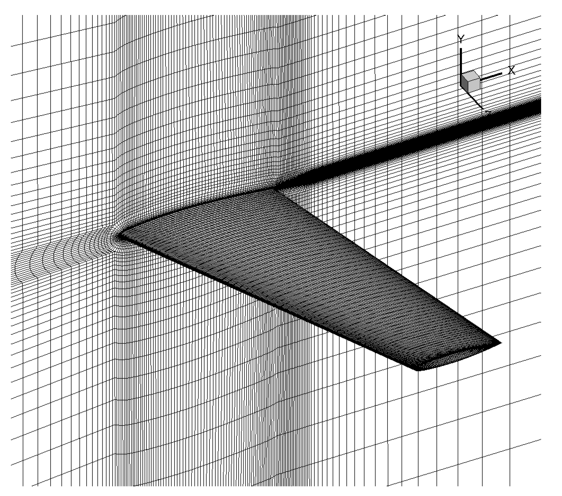
3.5. Transonic ONERA M6 3D Airfoil

To test the 3D prediction ability of the model, we conduct a calculation over the transonic ONERA M6 3D airfoil. It is a calibrate case of transition verification. Calculation proceeds with the mesh, as in Figure 20. It is a H-type topology, including 250,000 cells in total. Mach number is set to 0.8395, Reynolds number is set to 11.72 × 10${}^6$, and the angle of attack is ${3.06}^{\circ }$.

From the comparison of surface pressure coefficient shown in Figure 21, we can find that the results of SA-RF are almost the same as the SST-$\gamma$-$R{e}_{\theta }$ model, and a discrepancy appears in the SA-NN model.

Three situations of the airfoil are investigated, as shown in Figure 22. Generally, all of the models fit well with the experimental value. Compared with the results of the SA model, the pressure coefficient near the wingtip is a little smaller. SA-RF model performs basically the same with SST-$\gamma$-$R{e}_{\theta }$ model, while SA-NN predicts the transition situation earlier, leading to a deviation at the wingtip.

4. Conclusions and Future Works

We presented and developed a model for predicting the transition phenomena of turbulence flow by harnessing powerful machine-learning techniques. To test the performance of the model, a turbulence model was constructed by embedding an SA model with a model trained by SST-$\gamma$-$R{e}_{\theta }$ convergence data. The model was then applied to predict cases of different geometric profiles, Reynolds numbers and angles of attack. The results are quite promising. Without new data given, SA-NN and SA-RF can both successfully reproduce the results of the SST-$\gamma$-$R{e}_{\theta }$ model in a wide variety of different flow conditions from 2-D airfoils to 3-D transonic wings; thus, they exhibited a strong generalization ability and can give promising prediction on flow fields. In addition, the adaptation of the two coupled models decrease computational cost to a great extent. The potential of machine-learning to act as a strong supplement to previous turbulence transition models is revealed in this work.

Further work will focus on integrating physical constraints and the adaptation of machine-learning algorithms. At present, the biggest challenge is feature selection. The investigations into the physics of the turbulence may offer new choices of finding input features to construct models with better performance. A RANS solver may not be represented until a model with enough richness to predict any important dynamics appears. Existing machine-learning turbulence models and expert domain knowledge provide a good starting point, and physical theories can further aid the process. In addition, research on the astringency and stability of the coupling system of the NS equation and machine-learning algorithms are needed for accelerating the convergence course of the model, and, thus, enhance calculation efficiency. Last but not least, the adaptation range of machine learning can broaden complicated transition problems in engineering, including the interaction between shock waves and the boundary layers, cross-flow instability and so on.