Article

In-Flight Radome Slope Estimation for Homing Guidance Using Bearing-Only Measurement via Gaussian Process Regression

1
School of Automation, Southeast University, Nanjing 210096, China
2
College of Automation Engineering, Nanjing University of Aeronautics and Astronautics, Nanjing 210016, China
3
Beijing Electro-Mechanical Engineering Institute, Beijing 100074, China
*
Author to whom correspondence should be addressed.
Aerospace 2022, 9(10), 626; https://doi.org/10.3390/aerospace9100626
Submission received: 11 August 2022 / Revised: 24 September 2022 / Accepted: 17 October 2022 / Published: 20 October 2022

Abstract

:
The radome refraction problem gives rise to guidance performance deterioration for homing missiles. Aiming to eliminate the effect of radome refraction on the radar seeker, a novel method is proposed for correcting the radome-induced measurement error by using the estimated guidance information. A dynamic model for the estimation system is formulated and the guidance information is estimated online via a multiple-model filtering framework. A Gaussian process regression scheme is introduced to reconstruct the mapping model with respect to the radome error and look angle. Furthermore, an analytical expression for radome slope estimation is derived by calculating the derivative of the surrogate function, represented with Gaussian process models. The contaminated measurement is corrected based on the estimated guidance information and radome slope. Extensive simulation results illustrate that the proposed method is able to estimate the radome slope accurately and improve the guidance accuracy effectively.

1. Introduction

The radome is employed for homing missiles [1] to protect the seeker antenna from air flow [2] and to reduce the aerodynamic drag as well [3]. The electromagnetic wave is not refracted by the radome when the shape of the radome is a perfect hemisphere [4]. However, for the reason that the aerodynamic drag force is excessively large in endo-atmospheric engagements, the radome is shaped to be non-hemispheric to reduce the drag [5] at the cost of inducing refraction of the electromagnetic wave [6]. The radome refraction phenomenon has a destabilizing effect on the missile-guidance system, as it results in measurement error in the line-of-sight (LOS) angle, so an unwanted feedback path is formulated in the homing guidance loop [7]. The proportional navigation (PN) guidance law [8] has been widely used due to its simplicity of implementation. The PN guidance law and its variants use LOS angle measurements for command generation [9], in which the acceleration command is calculated based on the closing velocity as well as the LOS angular rate obtained from the radar seeker [10]. For the reason that the homing performance of a guided missile [11] relies heavily on the sensing accuracy of the radar seeker, the radome refraction effect might cause severe degradation of the guidance accuracy [12]. While the radome refraction angle is usually not large in practical situations, its induced angular rate of change might cause guidance problems as it adds a parasitic feedback loop to the guidance system [13,14]. The effect of missile body disturbance on the gimbal phased array seeker is analyzed by formulating a disturbance rejection problem [15]. The influence of the parasitic loop on the rolling missile is also investigated, in which the dynamic system is modeled by employing a two-loop autopilot [16]. Furthermore, the analytical stability of the guidance system with consideration of the radome refraction effect is analyzed and the stability region of the guidance loop is studied in terms of a function of missile parameters [10] and a constant rate-based method is proposed to slow down the autopilot response to reduce the miss distance [17]. In this regard, it is necessary to develop a compensation method to mitigate the radome refraction effect for guidance performance enhancement.
Several radome compensation methods have been proposed in the literature. One kind of method is hardware based, which means a careful manufacture of the radome and a large amount of digital shifter used in the seeker [18]. Another one represents radome boresight error compensation [19], in which an approach using the radome aberration angle obtained from costly measuring instruments is proposed [20]. The last one is algorithmic based, in which the control theory is used to slow down the guidance loop response [17], the radome characteristics are approximated by applying neural network techniques [21] and the filtering technique [22] is used for error estimation and compensation [6]. These methods can be also divided into two categories: offline and online. The offline approaches aim to model the radome characteristics through analysis of experimental samples [23]. As the surrogate model is obtained, it is stored in the onboard computer for correcting the radome error in flight [24]. However, the radome characteristics modeled with a ground test might be deviated from in flight for the sake of aerodynamic heating [25]. To overcome the limitations of the offline approaches, online approaches are developed based on Bayesian filtering techniques [26]. A nonlinear filtering algorithm is proposed to decouple the radome error from the nominal missile states [2], in which a two-step estimator is implemented with measurements of the azimuth and elevation angles. State estimation algorithms with LOS angle measurements have been studied in various studies [4,12,27], in which the radome slope is estimated from the information generated by dither and extracted by bandpass filtering [28]. At the same time, the nonlinear filtering techniques [29] have practical limitations, including sensitivity to initial value, slow convergence and performance degradation in the presence of model parameter mismatch [6]. To make up the flaws of the nonlinear filters, an estimator using a multiple-model-based scheme is proposed [30]. In addition, by assuming that the radar seeker provides range and LOS angle measurements, the interactive multiple-model method was studied [31]. The observability of the dynamic systems is supposed to be guaranteed for accurate state estimation. However, when the range information is not available, it can lead to a deterioration of the estimation accuracy due to a lack of observability [3]. In this regard, a precise estimate of the radome slope has been recognized as a critical issue for the radome-induced error correction problem.
In order to overcome the poor observability problem for radome slope estimation [4] with LOS-angle-only measurements, a novel method is proposed in this work for online identification of radome slope by combining adaptive filtering and statistical learning techniques. The main contributions of this work are two-fold. On one hand, a Gaussian process regression (GPR) method is proposed to reconstruct the mapping relationship between the look angle and radome error. It is well known that a lack of prior information in modeling deteriorates the estimation accuracy of filtering algorithms; thus, it is more reliable to update the radome refraction model persistently by incorporating real-time data, instead of performing model-based Bayesian filtering directly under the risk of model mismatch. On the other hand, an analytical expression is obtained for radome slope estimation by deriving the derivative of the mapping function represented with a Gaussian process model. Existing methods [4,32] often treat the unknown radome slope as a state variable and approximate it with a random walk model. However, the parameter of the surrogate model, i.e., the variance, is difficult to determine in practice. Based on this fact, the proposed radome slope estimation method is more accurate as its calculation formula is derived based on the original definition without approximation error. In addition, the statistical feature of probabilistic modeling and analysis makes GPR a reliable tool for physics-informed estimation. Through extensive simulations, it is shown that the guidance performance can be improved by using the estimated radome slope for LOS angular rate correction. The rest of this paper is organized as follows. In Section 2, the guidance system and engagement kinematics are introduced and a mathematical model of the radome refraction phenomenon is formulated. In Section 3, the problem of radome slope estimation is studied based on adaptive filtering and statistical learning. Extensive simulations are conducted to analyze the effectiveness of the LOS angular rate corrector in Section 4. The overall conclusion of this paper is delivered in Section 5.

2. Problem Formulation

The radar antenna is placed in the missile seeker for target tracking, such that the LOS angle is obtained to generate missile-guidance command. In endo-atmospheric engagements, the radome is required to protect the radar antenna from air flow. At the same time, it can be observed from Figure 1 that a radio wave is refracted when it passes through the radome, which makes the tracked target appear to be displaced from its true position due to radome refraction [32].
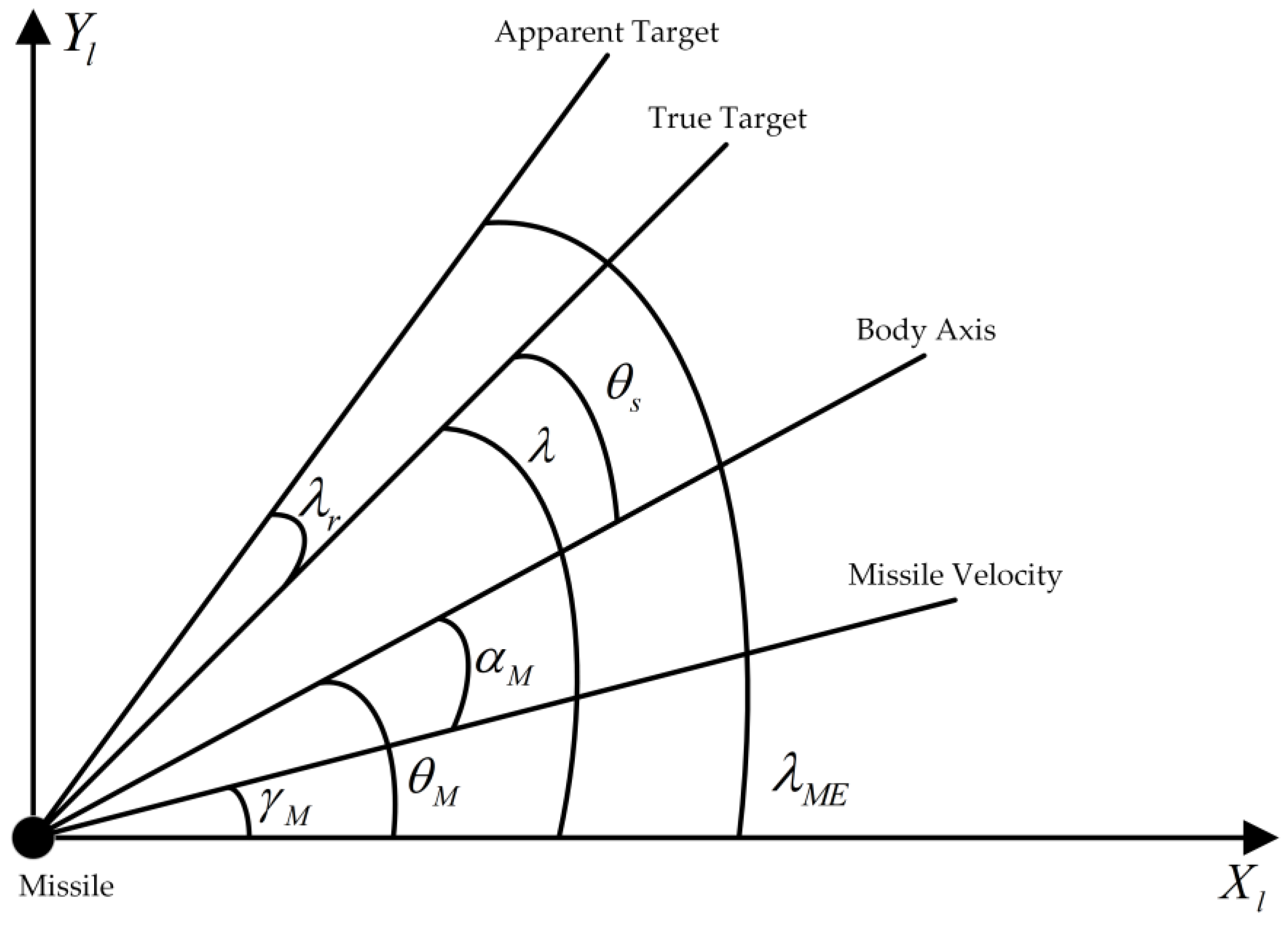
The engagement geometry between the missile and target is shown in Figure 2 in the inertial Cartesian coordinate system [4], where γ M , θ M , θ s and α M are flight path angle, body pitch angle, look angle and angle of attack for the missile, respectively. In addition, λ r and λ represent the radome error and the LOS angle. According to Figure 2, the measured LOS angle, which is contaminated due to radome refraction, is formulated as
λ M E λ + λ r
in which the radome error λ r is modeled according to ref. [2,4] in terms of a function of look angle θ s as follows
λ r = f λ r ( θ s ) θ s λ θ M
From Equations (1) and (2), the contaminated LOS angle λ M E is expressed as
λ M E = λ + f λ r ( λ θ M )
The guidance command A c m d using the PN guidance law is given as
A c m d = N × | R ˙ | × λ ˙ M E
where N denotes the navigation constant and R ˙ is the closing velocity. According to Equation (3), the contaminated LOS angular rate λ ˙ M E can be written as
λ ˙ M E = d λ d t + d f λ r ( λ     θ M ) d t = d λ d t + d f λ r ( λ     θ M ) d ( λ     θ M ) × d ( λ     θ M ) d t = λ ˙ + ρ θ × ( λ ˙     θ ˙ M )
where ρ θ denotes the radome slope, a parameter which represents the refraction characteristics of a certain radome. Substituting Equation (5) into Equation (4), the resulting guidance law becomes
A c m d = N × | R ˙ | × λ ˙ M E = N × | R ˙ | × ( λ ˙ + ρ θ × ( λ ˙ θ ˙ M ) )
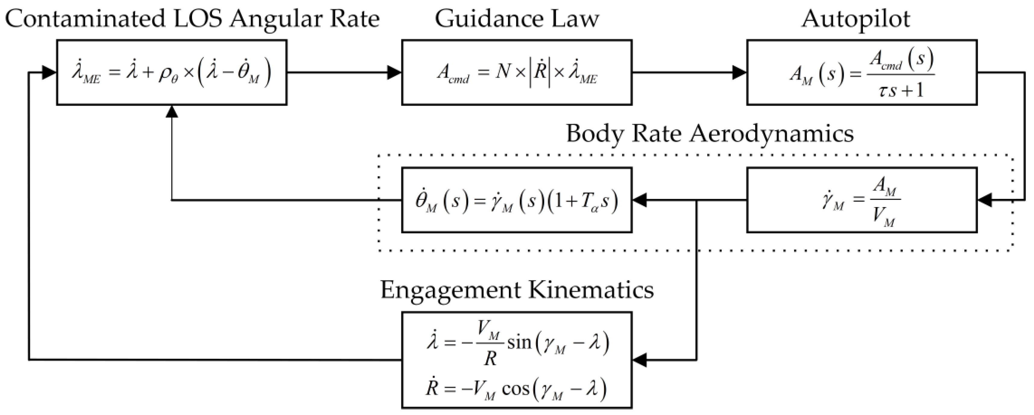
On account of the above relations, a system block diagram of the PN guidance system considering the radome refraction effect is formulated in Figure 3, as follows, in which the missile autopilot is modeled as a first-order lag system as
A M ( s ) A c m d ( s ) = 1 τ s + 1
The dynamics of the missile pitch angle are modeled in the form of a transfer function, given as
θ ˙ M ( s ) A M ( s ) = 1 + T α s V M
in which V M represents the missile velocity. In addition, the target is assumed to be stationary [4]; thus, as shown in Figure 4, the engagement kinematics between the missile and target are modeled in the polar coordinate system, given as
λ ˙ = V M R sin ( γ M λ ) R ˙ = V M cos ( γ M λ )
It can be observed from Figure 3 that the radome slope ρ θ induces the missile seeker to generate a contaminated LOS angular rate λ ˙ M E . Then, the signal λ ˙ M E passes through the guidance computer and the autopilot to generate an erroneous acceleration command A M , which results in unnecessary attitude movement of the missile body. In this manner, a parasitic loop [33] is formed in the guidance system that couples the pitch angular rate θ ˙ M with the contaminated LOS angular rate λ ˙ M E obtained from the missile seeker. The consequence of the radome refraction effect is an increase in miss distance as it causes the missile flight system to respond in an erroneous way [18]. Furthermore, the parasitic loop is destabilizing to the guidance system and the stability problem becomes more severe when the value of the radome slope exceeds a permissible range [21,28]. This fact reveals that it is necessary to design an in-flight measurement error calibration system to overcome the problem imposed by radome refraction. To this end, the aim of this paper is to develop a novel method to estimate the radome slope and correct the measurement information in the guidance system.

3. Radome Slope Estimation and Compensation

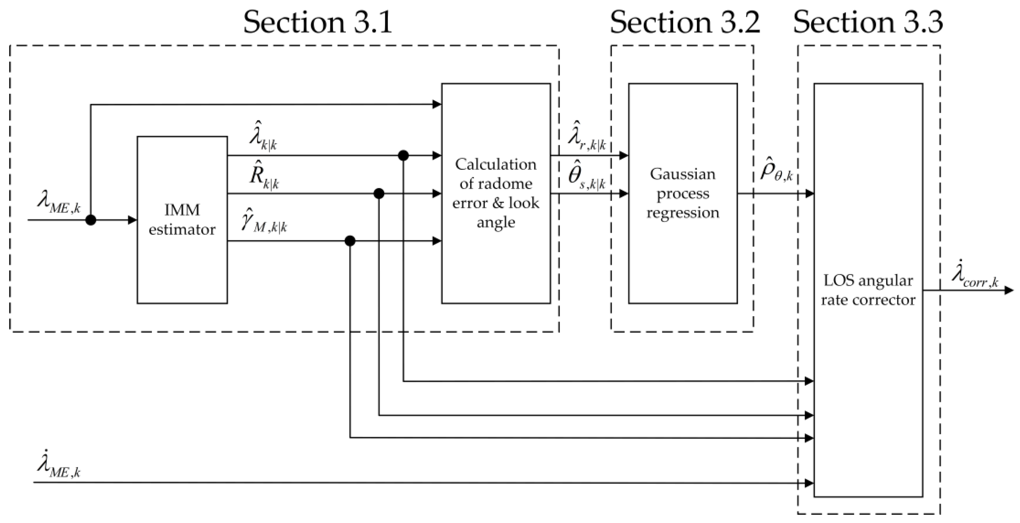
In this section, the problem of radome slope estimation is studied based on adaptive filtering and statistical learning. A multiple-model filtering framework is constructed to estimate the guidance information by using LOS angle measurements. After that, a Gaussian process regression scheme is proposed to reconstruct the mapping relationship between the look angle and radome error. Furthermore, an analytical expression is obtained to estimate the radome slope by deriving the derivative of the mapping function, represented by Gaussian process models. In the end, the LOS angular rate corrector is implemented by using the estimated radome slope to mitigate the radome refraction effect. To this end, a system block diagram of the PN guidance system with LOS angular rate corrector incorporated in the loop is presented in Figure 5.

3.1. Guidance Information Estimation Using IMM Filter

While the radome error cannot be measured directly, a filtering approach is proposed for state estimation of the engagement kinematics observed by the missile seeker. Next, the radome error is analytically inferred by using the estimated guidance information and the measured LOS angle. In the proposed filter, it consists of LOS angle λ , relative distance R and flight path angle γ M as state variables to be estimated. With this consideration, a dynamic model of the estimation system is constructed as
x ˙ = f ( x , u )
in which x = ( x 1 , x 2 , x 3 ) T ( λ , R , γ M ) T denote the system state, u A M represents the maneuver acceleration of the missile as input and the dynamic model (10) is formed as
d λ d t = V M R sin ( γ M λ ) d R d t = V M cos ( γ M λ ) d γ M d t = u V M
After that, the continuous-time dynamic equations introduced in Equation (11) are discretized using a 4th-order Runge–Kutta method [34]; thus, the time propagation of state variables at the k th step is expressed as
x k + 1 = ϕ ( x k , u k ; Δ t ) + w k
in which x k = ( x 1 , k , x 2 , k , x 3 , k ) T ( λ k , R k , γ M , k ) T denote the discretized system state at the k th time step, ϕ ( · , · ; · ) represents the state transition function and Δ t is the step size of the discretization. In addition, w k N ( 0 , Q ) is the process noise to account for discretization error and Q is its corresponding covariance matrix.
As the angle of attack is assumed to be negligible during terminal homing guidance [4], the LOS angle measurement is given from Figure 2 as follows
z k λ M E , k = h ( x k ; ρ θ , k ) = ( 1 + ρ θ , k ) λ k ρ θ , k γ M , k
in which ρ θ , k denotes the radome slope at the k th time step.
It can be observed from Equation (13) that the radome slope functions as a critical parameter for the measurement model. However, the actual value of the radome slope is, indeed, unknown. In this regard, an adaptive filtering approach using interacting multiple-model (IMM) structure is proposed to solve this issue, in which it constructs multiple hypotheses about the radome slope and runs parallel filtering models in a simultaneous manner.
Let the unknown parameter, namely the radome slope, be typified by a set of predetermined values as
P θ = { ρ θ 1 , ρ θ 2 , , ρ θ n }
in which n denotes the size of the set. Then, for each parameter value ρ θ i given in Equation (14), one can define its corresponding measurement model as
z k i = h ( x k ; ρ θ i )   for   i = 1 , n
and formulate a specific local filter by using the measurement model given in Equation (15) for state estimation. As a result, the IMM structure is constructed with a bank of n local filters, constituting a hybrid system designated by a parameter set, which contains n guessed radome slope values. In detail, one cycle of the IMM filtering algorithm consists of the following [35]:
The probability that ρ θ i was in effect at the ( k 1 ) th time step given that ρ θ j is in effect at the k th time step conditioned on Z k 1 { z 1 , , z k 1 } is
μ k 1 | k 1 i | j = 1 c ¯ j p i j μ k 1 i
in which μ k 1 | k 1 i | j denotes the mixing probability, p i j represents the ( i th , j th ) element of a given transition probability matrix π and μ k 1 i is the probability for the i th model. In addition, the normalizing constant c ¯ j is calculated as
c ¯ j = i = 1 n p i j μ k 1 i
Starting with x ^ k 1 | k 1 i , one computes the mixed initial condition for the filter matched to ρ θ j as
x ^ k 1 | k 1 0 j = i = 1 n x ^ k 1 | k 1 i μ k 1 | k 1 i | j
The covariance corresponding to the above is
P k 1 | k 1 0 j = i = 1 n μ k 1 | k 1 i | j ( P k 1 | k 1 i + ( x ^ k 1 | k 1 i x ^ k 1 | k 1 0 j ) ( x ^ k 1 | k 1 i x ^ k 1 | k 1 0 j ) T )
In this work, the unscented Kalman filter (UKF) [36] is used for local filtering, in which the estimate x ^ k 1 | k 1 0 j and covariance P k 1 | k 1 0 j are used as input to the filter matched to ρ θ j , which uses z k to yield x ^ k | k j and P k | k j . In detail, the operations of UKF are performed as follows:
Firstly, form the sigma points for the prediction step of UKF
χ k 1 ( 0 ) = x ^ k 1 | k 1 0 j χ k 1 ( l ) = x ^ k 1 | k 1 0 j + 3 + λ [ P k 1 | k 1 0 j ] l χ k 1 ( l + 3 ) = x ^ k 1 | k 1 0 j 3 + λ [ P k 1 | k 1 0 j ] l   for   l = 1 , 2 , 3
in which λ is a scaling parameter given as λ α 2 ( 3 + κ ) 3 , the parameters α and κ determine the spread of the sigma points around the mean. Note that the matrix square root denotes a matrix, such that P k 1 | k 1 0 j ( P k 1 | k 1 0 j ) T = P k 1 | k 1 0 j and [ · ] l denotes the l th column of the matrix.
After that, propagate the sigma points through the dynamic model
χ ^ k ( l ) = ϕ ( χ k 1 ( l ) )   for l = 0 , 1 , , 6
Compute the predicted mean x ^ k | k 1 j and the predicted covariance P k | k 1 j
x ^ k | k 1 j = l = 0 6 W l ( m ) χ ^ k ( l ) P k | k 1 j = l = 0 6 W l ( c ) ( χ ^ k ( l ) x ^ k | k 1 j ) ( χ ^ k ( l ) x ^ k | k 1 j ) T + Q
in which the weights W l ( m ) and W l ( c ) are defined as follows
W 0 ( m ) = λ 3   +   λ W 0 ( c ) = λ 3   +   λ + ( 1 α 2 + β )
where β is a parameter that can be used for incorporating prior information and
W l ( m ) = W l ( c ) = 1 2 × ( 3 + λ )   for l = 0 , 1 , , 6
Secondly, form the sigma points for the correction step of UKF
χ k ( 0 ) = x ^ k | k 1 j χ k ( l ) = x ^ k | k 1 j + 3 + λ [ P k | k 1 j ] l χ k ( l + 3 ) = x ^ k | k 1 j 3 + λ [ P k | k 1 j ] l   for l = 1 , 2 , 3
After that, propagate sigma points through the measurement model
Z ^ k ( l ) = h ( χ k ( l ) )   for l = 0 , 1 , , 6
Compute the predicted mean z ^ k | k 1 j , the residual covariance S k j and the cross-covariance C k j of the state and the measurement
z ^ k | k 1 j = l = 0 6 W l ( m ) Z ^ k ( l ) S k j = l = 0 6 W l ( c ) ( Z ^ k ( l ) z ^ k | k 1 j ) ( Z ^ k ( l ) z ^ k | k 1 j ) T C k j = l = 0 6 W l ( c ) ( χ k ( l ) x ^ k | k 1 j ) ( Z ^ k ( l ) z ^ k | k 1 j ) T
Compute the filter gain, the filtered state mean and the covariance, conditional on the measurement
K k j = C k j ( S k j ) 1 x ^ k | k j = x ^ k | k 1 j + K k j ( z k z ^ k | k 1 j ) P k | k j = P k | k 1 j K k j S k j ( K k j ) T
In this regard, the operations of UKF are introduced from Equation (20) to Equation (28). In addition, the measurement residual ν k j z k z ^ k | k 1 j and residual covariance S k j are calculated, respectively, for each local filter to obtain the likelihood Λ k j of the corresponding hypothesis, namely
Λ k j = N ( ν k j ; 0 , S k j )
After that, the model probabilities are calculated as follows:
μ k j = 1 c Λ k j c ¯ j
in which c j = 1 n Λ k j c ¯ j is the normalization constant for Equation (30).
Finally, the state estimate is calculated with a combination of the model-conditioned means and covariances according to a mixture equation as
x ^ k | k = j = 1 n μ k j x ^ k | k j P k | k = j = 1 n μ k j ( P k | k j + ( x ^ k | k j x ^ k | k ) ( x ^ k j x ^ k | k ) T )
in which x ^ k | k and P k | k represent the estimated mean and covariance at the k th step, x ^ k | k j and P k | k j denote the local estimate obtained from the j th local filter and μ k j is its corresponding model probability at the k th step. In summary, the structure of the IMM estimator is shown in Figure 6, as follows.
Furthermore, let x ^ k | k = ( x ^ 1 , k | k , x ^ 2 , k | k , x ^ 3 , k | k ) T ( λ ^ k | k , R ^ k | k , γ ^ M , k | k ) T denote the estimated mean, then the estimated radome error λ ^ r , k | k can be calculated based on the engagement geometry shown in Figure 2, as follows
λ ^ r , k | k = λ ^ ME , k λ ^ k | k = z k λ ^ k | k
In addition, by assuming that the angle of attack is negligible during terminal homing guidance [4], the estimated look angle θ ^ s , k | k can be calculated in a similar manner as
θ ^ s , k | k = λ ^ k | k γ ^ M , k | k
In this regard, both the radome error λ ^ r , k | k and the look angle θ ^ s , k | k can be computed analytically with the estimated guidance information x ^ k | k and the measurement z k by using IMM filtering techniques. In the next section, a statistical learning-based approach is developed to explore the correlation between the radome error and look angle for radome slope estimation.

3.2. Radome Slope Estimation via Gaussian Process Regression

While the actual form of function f λ r ( · ) in Equation (2) is unknown to the guidance system, the aim of this part is to propose a machine-learning-based radome slope estimation method. In the following, by defining v r , i N ( 0 , r r , i ) as a deviation between the actual radome error λ r , i and the estimated radome error λ ^ r , i | i at the i th time step, we see that
λ ^ r , i | i = λ r , i + v r , i   for   i [ i 1 , i 2 ]
where i 1 and i 2 denote the index of the starting and ending time steps for training data generation, respectively. Consider that the estimation error of look angle is negligible, i.e., θ ^ s , i | i θ s , i 0 , then the actual radome error λ r , i is expressed based on Equation (2) as
λ r , i = f λ r ( θ ^ s , i | i )
Substituting Equation (35) into Equation (34), a mathematical relation between θ ^ s , i | i and λ ^ r , i | i is formulated as follows
λ ^ r , i | i = f λ r ( θ ^ s , i | i ) + v r , i
From Equation (36), it can be seen that λ ^ r , i | i represents a noisy version of the output for function f λ r ( · ) with its input given as θ ^ s , i | i . Next, consider an arbitrary input denoted by θ ^ s , j | j , then the mapping from the input θ ^ s , j | j to the output λ r , j is written similarly to Equation (35) as
λ r , j = f λ r ( θ ^ s , j | j )
For the reason that the function f λ r ( · ) is unknown, it requires one to estimate the value of f λ r ( θ ^ s , j | j ) based on θ ^ s , j | j by using available mapping pairs { ( θ ^ s , i | i , λ ^ r , i | i ) } i = i 1 i 2 as training data. One issue that comes from this concern is how to establish a reasonable correlation between the training data and the unknown mapping pair ( θ ^ s , j | j , f λ r ( θ ^ s , j | j ) ) , due to the reason that without supplementary assumptions, the values of f λ r ( θ ^ s , j | j ) and { λ ^ r , i | i } i = i 1 i 2 are isolated. In this regard, assume that the function f λ r ( · ) is smooth, then from a probabilistic point of view, all the outputs generated from function f λ r ( · ) become correlated, in which the prior correlation between the two arbitrary outputs f λ r ( x 1 ) and f λ r ( x 2 ) is represented with a squared exponential covariance function [37], denoted as
k ( x 1 , x 2 ) α 2 exp ( ( x 1 x 2 ) 2 2 Λ )
in which k ( · , · ) denotes a kernel function, α is a constant used to scale the standard deviation and Λ is used to scale the input variables. In the following, Equation (34) is rewritten in vector form for notational simplicity as
λ r i = λ ^ r i v r i   for   i [ i 1 , i 2 ]
in which
λ r i ( λ r , i 1 λ r , i 2 ) = ( f λ r ( θ ^ s , i 1 | i 1 ) f λ r ( θ ^ s , i 2 | i 2 ) )
λ ^ r i ( λ ^ r , i 1 | i 1 λ ^ r , i 2 | i 2 )
and v r i N ( 0 , R r i ) with R r i ( r r , i 1 0 0 0 0 0 0 r r , i 2 ) . Provided that the estimates of the outputs for function f λ r ( · ) are modelled as Gaussian random variables, the prior estimates of λ r i and λ r , j are set up to be jointly Gaussian, distributed as
( λ r i λ r , j ) N ( ( m i m j ) , ( K i + R r i K i , j K j , i K j ) )
where m i ( m i 1 , , m i 2 ) T and m j denote the prior means for λ r i and λ r , j , respectively. In addition, the components of the covariance matrix in Equation (42) are obtained as follows
K i ( k ( θ ^ s , i 1 | i 1 , θ ^ s , i 1 | i 1 ) k ( θ ^ s , i 1 | i 1 , θ ^ s , i 2 | i 2 ) k ( θ ^ s , i 2 | i 2 , θ ^ s , i 1 | i 1 ) k ( θ ^ s , i 2 | i 2 , θ ^ s , i 2 | i 2 ) )
K i , j ( k ( θ ^ s , i 1 | i 1 , θ ^ s , j | j ) k ( θ ^ s , i 2 | i 2 , θ ^ s , j | j ) )
K j , i ( k ( θ ^ s , j | j , θ ^ s , i 1 | i 1 ) , , k ( θ ^ s , j | j , θ ^ s , i 2 | i 2 ) )
K j k ( θ ^ s , j | j , θ ^ s , j | j )
In this regard, we are able to calculate the posterior distribution of λ r , j conditioned on λ r i . By using the Gaussian process regression scheme, the conditional density p ( λ r , j | λ r i ) is derived as
p ( λ r , j | λ r i ) N ( η j , j )
with
η j = m j + K j , i ( K i + R r i ) 1 ( λ ^ r i m i )
j = K j K j , i ( K i + R r i ) 1 K i , j
As a result, consider an arbitrary input denoted as θ ^ s , j | j ; it is able to estimate the corresponding output value for function f λ r ( · ) by using training data { ( θ ^ s , i | i , λ ^ r , i | i ) } i = i 1 i 2 . According to Equations (47)–(49), η j represents the mean value of the estimated output. In addition, j can be used to quantify the uncertainty with respect to the estimated output. As the mapping function from the look angle to the radome error is formulated with a Gaussian process regression scheme, the remaining work to be conducted is to investigate the derivative of the mapping function, i.e., to estimate the radome slope d η j d θ ^ s , j | j based on the same training data. From Equation (48), it can be observed that only the K j , i term depends on the input point θ ^ s , j | j ; therefore, to calculate the slope of the posterior mean, it just requires one to differentiate the kernel. For the squared exponential covariance function introduced in Equation (38), the derivate of the kernel between θ ^ s , j | j and a training point θ ^ s , i | i is derived as follows
d k ( θ ^ s , j | j , θ ^ s , i | i ) d θ ^ s , j | j = d d θ ^ s , j | j ( α 2 exp ( ( θ ^ s , j | j θ ^ s , i | i ) 2 2 Λ ) ) = d d θ ^ s , j | j ( ( θ ^ s , j | j θ ^ s , i | i ) 2 2 Λ ) α 2 exp ( ( θ ^ s , j | j θ ^ s , i | i ) 2 2 Λ ) = θ ^ s , j | j θ ^ s , i | i Λ k ( θ ^ s , j | j , θ ^ s , i | i )
Recall that K j , i ( k ( θ ^ s , j | j , θ ^ s , i 1 | i 1 ) , , k ( θ ^ s , j | j , θ ^ s , i 2 | i 2 ) ) , as introduced in Equation (45), then it can be written that
d K j , i d θ ^ s , j | j = ( θ ^ s , j | j θ ^ s , i 1 | i 1 Λ k ( θ ^ s , j | j , θ ^ s , i 1 | i 1 ) θ ^ s , j | j θ ^ s , i 2 | i 2 Λ k ( θ ^ s , j | j , θ ^ s , i 2 | i 2 ) ) T
and the slope of the posterior mean is written as
d η j d θ ^ s , j | j = d K j , i d θ ^ s , j | j ( K i + R r i ) 1 ( λ ^ r i m i ) = 1 Λ ( ( θ ^ s , j | j θ ^ s , i 1 | i 1 ) k ( θ ^ s , j | j , θ ^ s , i 1 | i 1 ) ( θ ^ s , j | j θ ^ s , i 2 | i 2 ) k ( θ ^ s , j | j , θ ^ s , i 2 | i 2 ) ) T ( K i + R r i ) 1 ( λ ^ r i m i )
Define θ ˜ s , j i ( θ ^ s , j | j θ ^ s , i 1 | i 1 , , θ ^ s , j | j θ ^ s , i 2 | i 2 ) T , then Equation (52) can be rewritten as
d η j d θ ^ s , j | j = 1 Λ ( ( θ ^ s , j | j θ ^ s , i 1 | i 1 ) ( θ ^ s , j | j θ ^ s , i 2 | i 2 ) ) T ( ( k ( θ ^ s , j | j , θ ^ s , i 1 | i 1 ) k ( θ ^ s , j | j , θ ^ s , i 2 | i 2 ) ) ( ( K i + R r i ) 1 ( λ ^ r i m i ) ) ) = 1 Λ ( θ ˜ s , j i ) T ( ( K j , i ) T ( ( K i + R r i ) 1 ( λ ^ r i m i ) ) )
where represents an element-wise product. In this regard, it is able to estimate the derivative of the posterior mean of a Gaussian process model. In other words, for an arbitrary input look angle θ ^ s , j | j , its corresponding radome slope ρ ^ θ , j is estimated as
ρ ^ θ , j d η j d θ ^ s , j | j = 1 Λ ( θ ˜ s , j i ) T ( ( K j , i ) T ( ( K i + R r i ) 1 ( λ ^ r i m i ) ) )
in which j denotes the j th time step, θ ˜ s , j i ( θ ^ s , j | j θ ^ s , i 1 | i 1 , , θ ^ s , j | j θ ^ s , i 2 | i 2 ) T , i 1 and i 2 are set up according to different implementation schemes.

3.3. Implementation of the LOS Angular Rate Corrector

This section deals with algorithm implementation for LOS angular rate correction in the guidance loop, in which the estimated radome slope obtained from Equation (54) is used to correct the contaminated LOS angular rate λ ˙ M E , such that the radar seeker provides precise measurement information for guidance law generation in real time. To this end, the form of the LOS angular rate corrector is constructed as follows
λ ˙ c o r r , k = 1 1 + ρ ^ θ , k λ ˙ M E , k + ρ ^ θ , k 1 + ρ ^ θ , k θ ˙ M , k
in which ρ ^ θ , k denotes the estimated radome slope calculated via Gaussian process regression, λ ˙ M E , k represents the contaminated LOS angular rate and θ ˙ M , k denotes the estimated pitch angular rate of the missile. Note that according to Equation (5), the contaminated LOS angular rate is able to be expressed as
λ ˙ M E , k = λ ˙ k + ρ θ , k × ( λ ˙ k θ ˙ M , k )
By substituting Equation (56) into Equation (55), we obtain
λ ˙ c o r r , k = λ ˙ k   +   ρ θ , k ( λ ˙ k     θ ˙ M , k )   +   ρ ^ θ , k θ ˙ M , k 1   +   ρ ^ θ , k = 1   +   ρ ^ θ , k 1   +   ρ ^ θ , k λ ˙ k + ρ θ , k     ρ ^ θ , k 1   +   ρ ^ θ , k λ ˙ k + ρ ^ θ , k     ρ θ , k 1   +   ρ ^ θ , k θ ˙ M , k = λ ˙ k + ρ θ , k     ρ ^ θ , k 1   +   ρ ^ θ , k ( λ ˙ k     θ ˙ M , k )
In this regard, it can be observed from Equation (57) that if ρ ^ θ , k 0 , which means that the LOS angular rate corrector is not activated, then the value of λ ˙ c o r r , k becomes
λ ˙ c o r r , k = λ ˙ k + ρ θ , k ( λ ˙ k θ ˙ M , k )
and this result is identical to λ ˙ M E , k , namely the contaminated LOS angular rate given in Equation (56). Furthermore, consider that the estimation result of the radome slope via Gaussian process regression is accurate, namely ρ θ , k ρ ^ θ , k 0 , then the value of λ ˙ c o r r , k becomes λ ˙ c o r r , k λ ˙ k , which means that the proposed LOS angular rate corrector formed in Equation (55) is able to output the true LOS angular rate λ ˙ k by using the estimated radome slope ρ ^ θ , k to eliminate the radome refraction effect. Note that the angle of attack is assumed to be negligible during terminal homing guidance [4]; thus, θ ˙ ^ M is able to be approximated with γ ˙ ^ M and we obtain
λ ˙ c o r r , k = 1 1   +   ρ ^ θ , k λ ˙ M E , k + ρ ^ θ , k 1   +   ρ ^ θ , k γ ˙ M , k = 1 1   +   ρ ^ θ , k λ ˙ M E , k + ρ ^ θ , k 1   +   ρ ^ θ , k u k V M
in which u k A M , k . As a result, the LOS angular rate corrector is implemented in discrete domain via Equation (59), in which the guidance information is obtained from the IMM filter and the radome slope is estimated via Gaussian process regression. In summary, a block diagram is presented to illustrate the proposed LOS angular rate corrector in Figure 7 and the corresponding pseudo code is summarized in Algorithm 1, as follows:
Algorithm 1: Pseudo code for the proposed LOS angular rate corrector at the kth time step.
Inputs: the contaminated LOS angle λ M E , k , the contaminated LOS angular rate λ ˙ M E , k
  1: calculate the estimated LOS angle λ ^ k | k and the estimated flight path angle γ ^ M , k via Equation (31)
  2: calculate the estimated radome error λ ^ r , k | k via Equation (32)
  3: calculate the estimated look angle θ ^ s , k | k via Equation (33)
  4: calculate the estimated radome slope ρ ^ θ , k via Equation (54)
  5: calculate the corrected LOS angular rate λ ˙ c o r r , k via Equation (59)
Output: the corrected LOS angular rate λ ˙ c o r r , k

4. Simulation

In this section, simulations are conducted to evaluate the proposed radome slope estimation and compensation method. First of all, the filtering accuracy of the IMM estimator is verified by conducting extensive simulations. Secondly, test cases are designed to evaluate the estimation accuracy of the unknown radome slope via Gaussian process regression. In the end, the effectiveness of the LOS angular rate corrector is verified in the guidance loop. The results of all the simulations are obtained via MATLAB R2021b in a PC with a CPU Intel Core i9 3.30 GHz and RAM of 64 GB. In the following simulation studies, the initial values of the missile and target states are given as
( X M , Y M , V M X , V M Y ) = ( 0   m , 0   m , 500   m / s , 0   m / s ) ( X T , Y T , V T X , V T Y ) = ( 10 4   m , 10 3   m , 0   m / s , 0   m / s )
where ( X M , Y M ) , ( X T , Y T ) denote initial positions of the missile and target, respectively. ( V M X , V M Y ) and ( V T X , V T Y ) denote the velocities of the missile as well as the target, in which the target is assumed to be stationary. In accordance with Equation (60), the initial state vector x ( 0 ) for the dynamic model in Equation (10) is given as
x ( 0 ) ( λ ( 0 ) , R ( 0 ) , γ M ( 0 ) , ) T = ( 0 . 0997   rad , 10,050   m , 0   rad ) T
and the corresponding model parameters are given as
{ V M , N , ρ θ , τ , T α } = { 500   m / s , 4 , 0.025 ° / ° , 0.1   s , 1   s }
For the IMM estimator, the step size of the discretized model is considered as Δ t = 1   ms and the transition probability matrix π of the Markovian chain is taken as
π = ( 0.9 0.05 0.05 0.05 0.9 0.05 0.05 0.05 0.9 )
In addition, the covariance Q of the process noise w k is given as
Q = ( 1.7453 2   ×   10 10   rad 2 0 0 0 500   m 2 0 0 0 1.7453 2   ×   10 10   rad 2 )
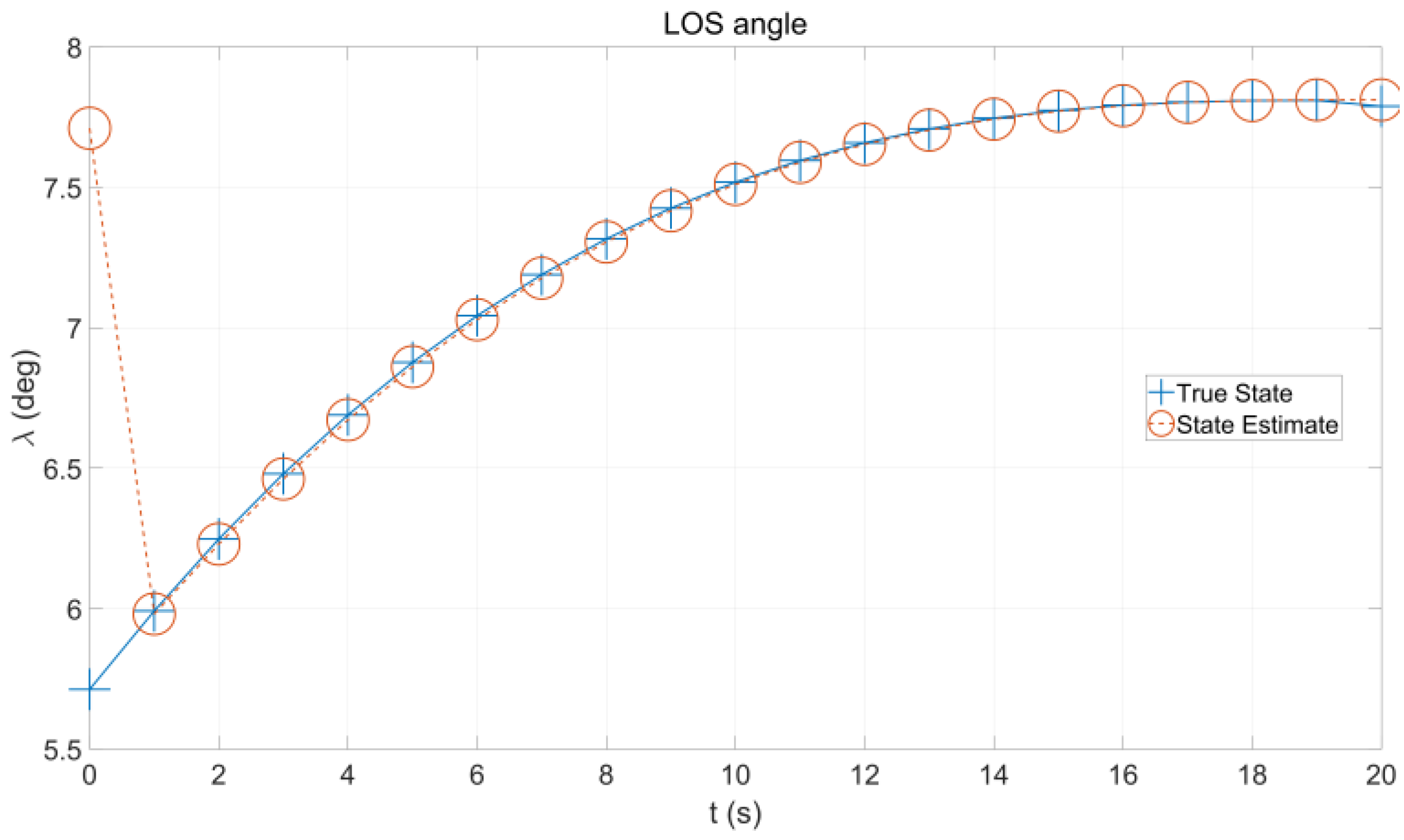
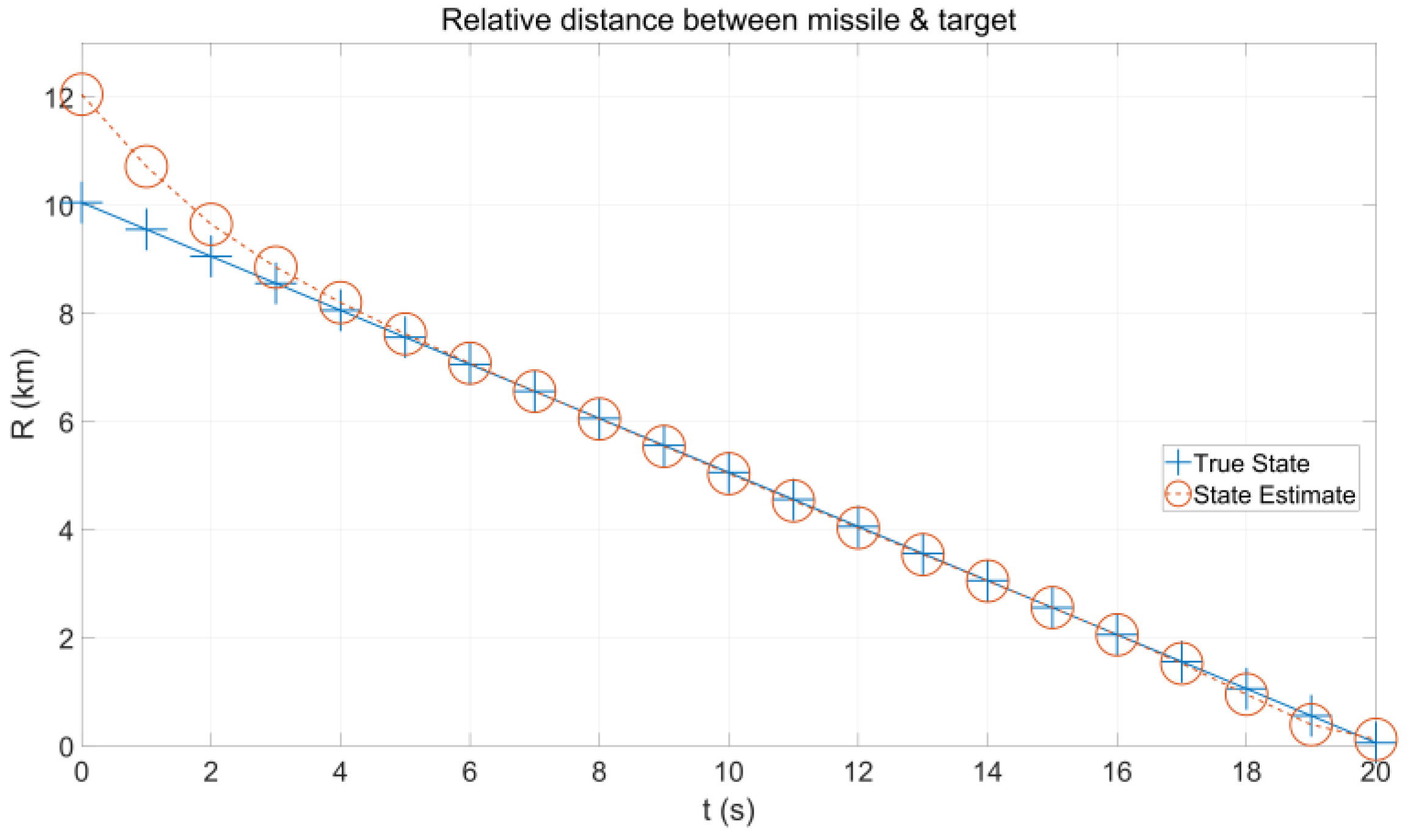
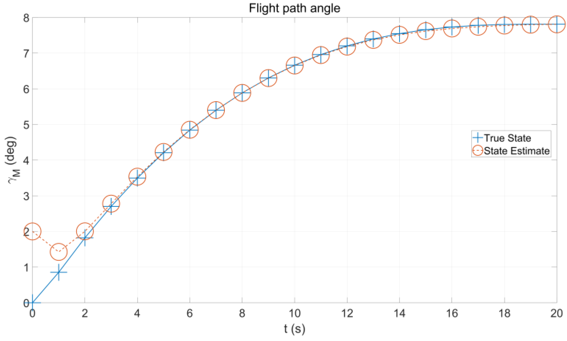
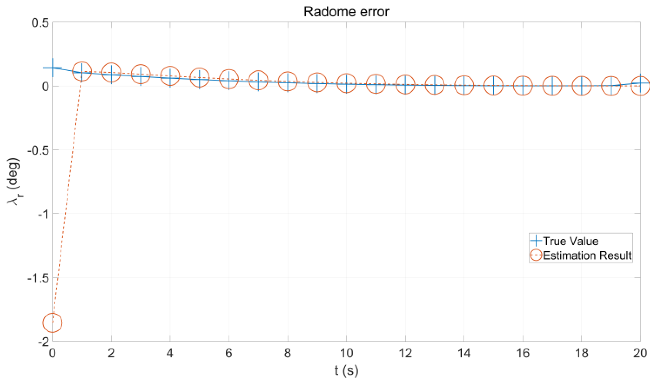
As shown in Figure 8, Figure 9 and Figure 10, the trajectories of the real system formed with Equation (10) and corresponding filtering results from the IMM estimator are presented. It can be seen from these figures that by applying the IMM estimator, while the estimation errors are relatively large at the early stage, they are gradually decreased and bounded in steady state as the missile moves close to the target. Furthermore, note that the estimated look angle and radome error are calculated according to Equations (32) and (33) by using the filtering results from the IMM estimator as well as the measurements from the seeker. It is observed from Figure 11 and Figure 12 that the deviations in these estimates from their true values gradually decreased over time, which suggests that the IMM estimator provides a satisfactory estimation result with respect to the guidance information. In this regard, it is able to investigate the correlation between the actual radome error and look angles by using the mapping pairs of the estimation result obtained from the IMM estimator as training data.
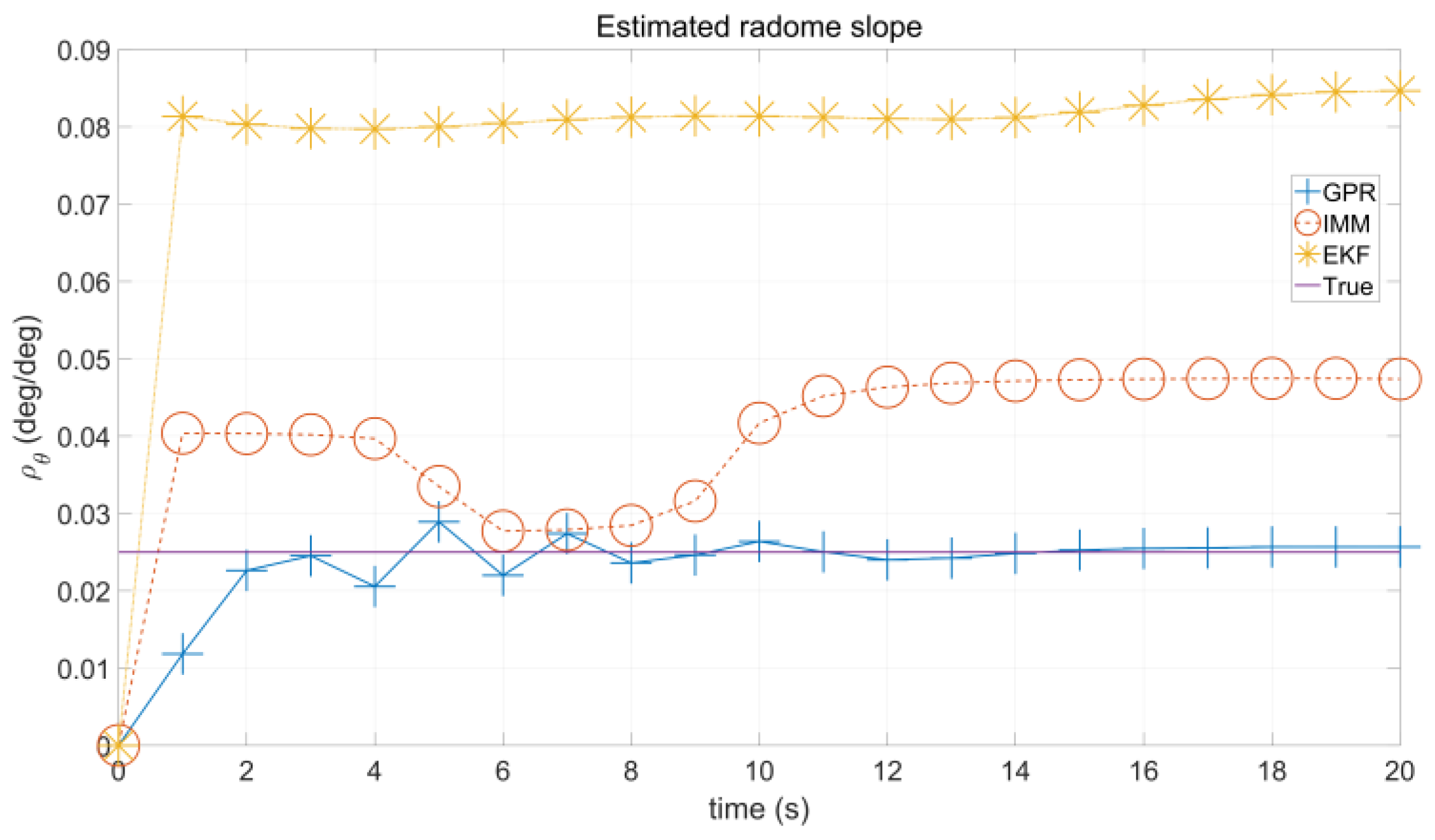
Next, the performance of the proposed GPR-based method introduced in Section 3.2 is evaluated for online radome slope estimation in the homing guidance loop. In detail, it considers that the training data used for regression are configured to be from the starting time step to the current time step. In another word, it supposes that the mapping pairs used for regression are given as { ( θ ^ s , i | i , λ ^ r , i | i ) } i = 1 k at time step k . Furthermore, the proposed GPR-based radome slope estimation method is compared with related works [4,38], in which the unknown radome slope is considered as system state and estimated directly via extended Kalman filter (EKF) and in another work the unknown radome slope is modeled to be system parameter and obtained as a weighted sum by using the IMM estimator. It can be seen from Figure 13 that the estimation accuracy of the proposed GPR-based method is superior to EKF and IMM for radome slope estimation, as its estimation result is mostly close to the true value, in which the actual radome slope ρ θ = 0.025 .
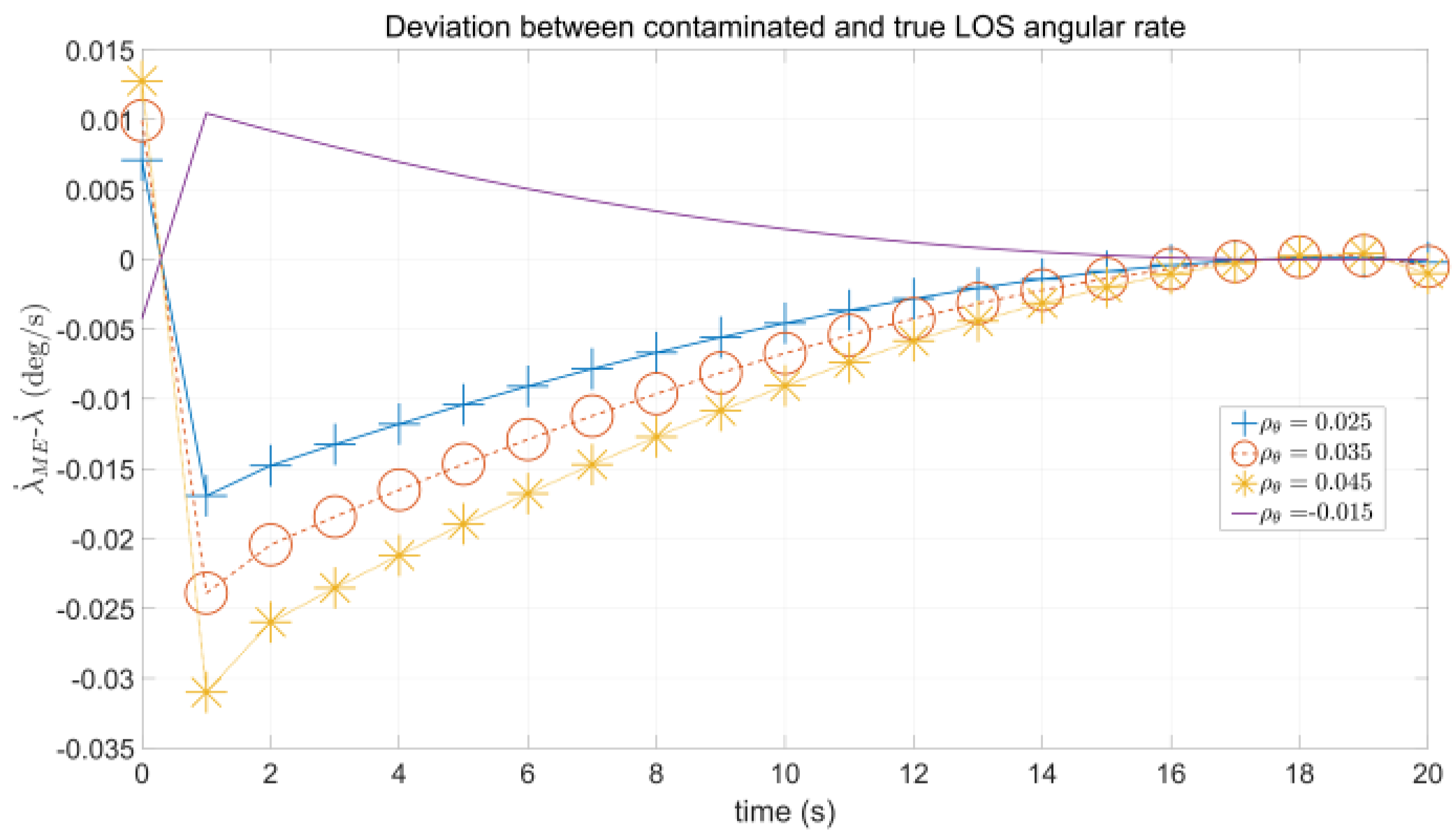
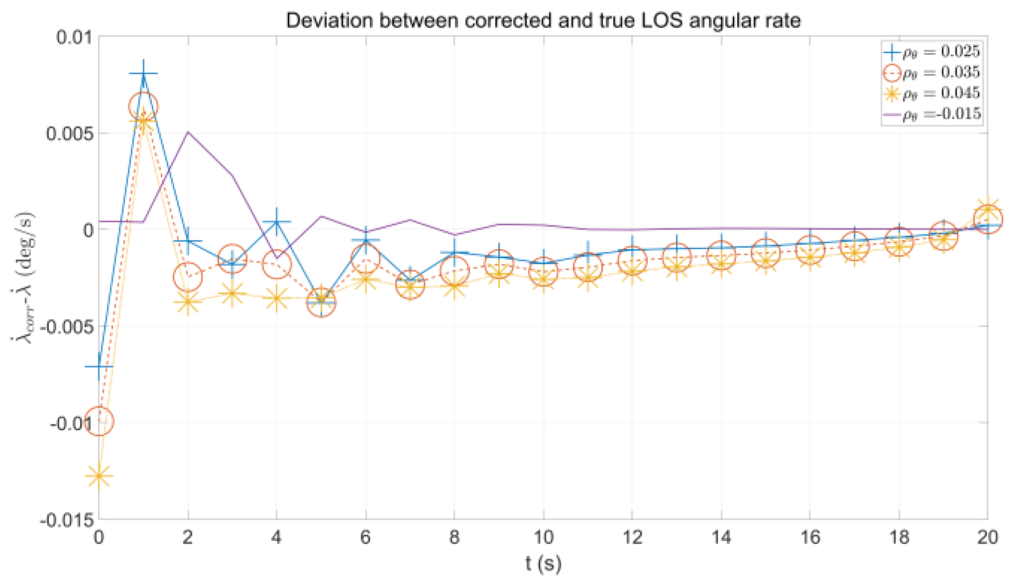
After that, simulations are carried out to evaluate the effectiveness of the LOS angular rate corrector proposed in Section 3.3, in which the estimated radome slope obtained via GPR is utilized in the guidance loop for compensation. For the implementation of the LOS angular rate corrector, a flowchart is presented in Figure 14, according to Equation (59). Firstly, the deviation between the contaminated LOS angular rate λ ˙ M E and the true LOS angular rate λ ˙ , i.e., λ ˙ M E λ ˙ , is calculated and presented in Figure 15 by varying the value of the radome slope ρ θ . It can be observed from this figure that the existence of the radome slope induces the missile seeker to generate a contaminated measurement. The value of λ ˙ M E λ ˙ is negative when ρ θ > 0 and the absolute value of it becomes larger with an increase of ρ θ . In addition, the value of λ ˙ M E λ ˙ becomes positive when ρ θ < 0 . For the reason that this deviation is nonnegligible, as the measurement from the missile seeker determines the value of the guidance command, it is necessary to correct the contaminated LOS angular rate λ ˙ M E by using the estimated radome slope ρ ^ θ . Secondly, the estimation error of the radome slope, namely ρ ^ θ ρ θ , is shown in Figure 16 by varying the value of the true radome slope. It can be seen from this figure that the GPR-based estimation method proposed in this work is effective as the estimation errors converge to zero in different cases. Lastly, the deviation between the corrected LOS angular rate λ ˙ c o r r and the true LOS angular rate λ ˙ , i.e., λ ˙ c o r r λ ˙ , is given in Figure 17. By comparing Figure 15 and Figure 17, it can be observed that the measurement error induced by radome refraction is alleviated with the help of the proposed LOS angular rate corrector, in which the values of λ ˙ c o r r λ ˙ are bounded in [ 0.005   deg / s , 0.005   deg / s ] when t 2   s , while at the same time, the values of λ ˙ M E λ ˙ are apparently larger.
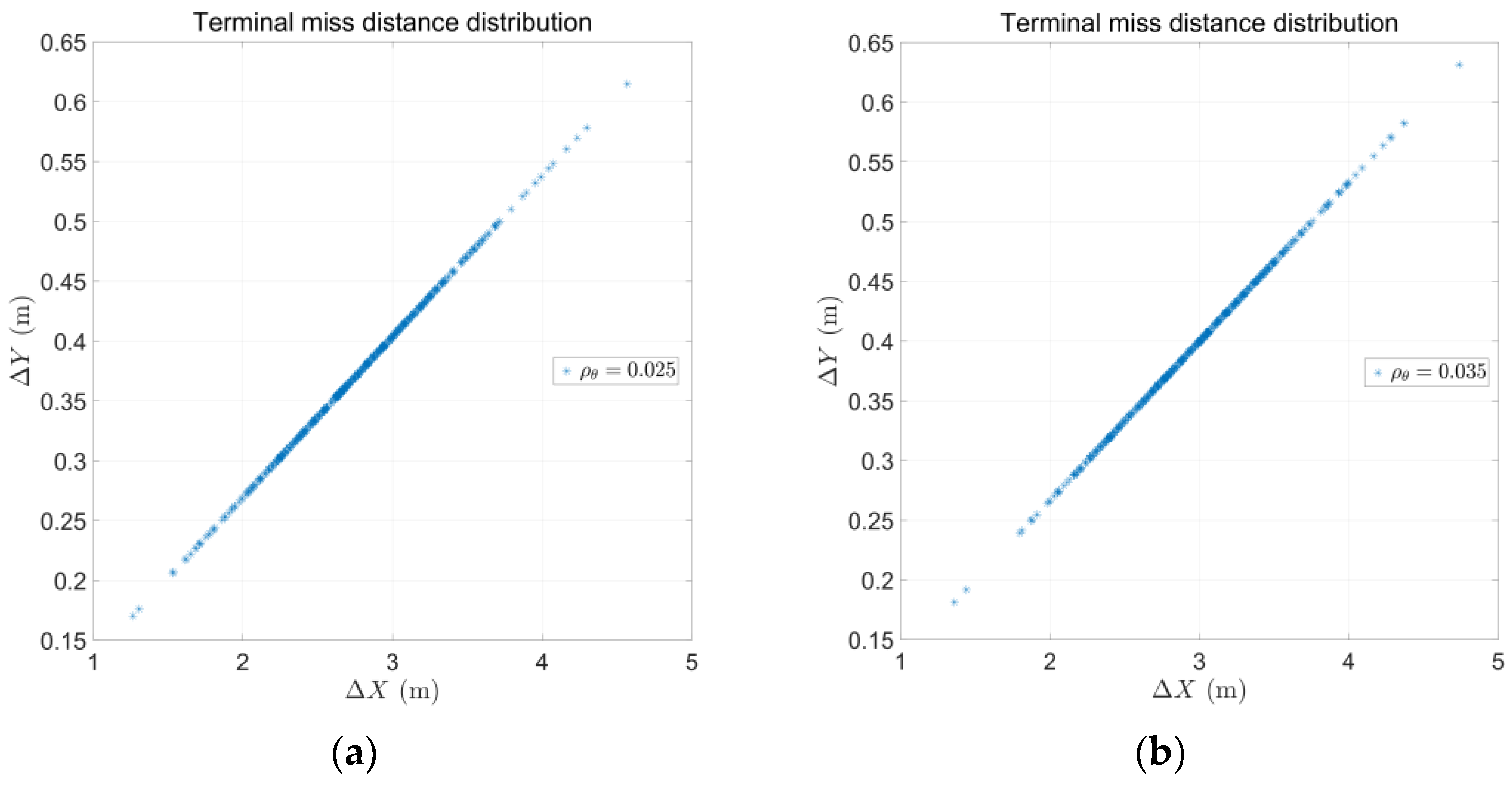
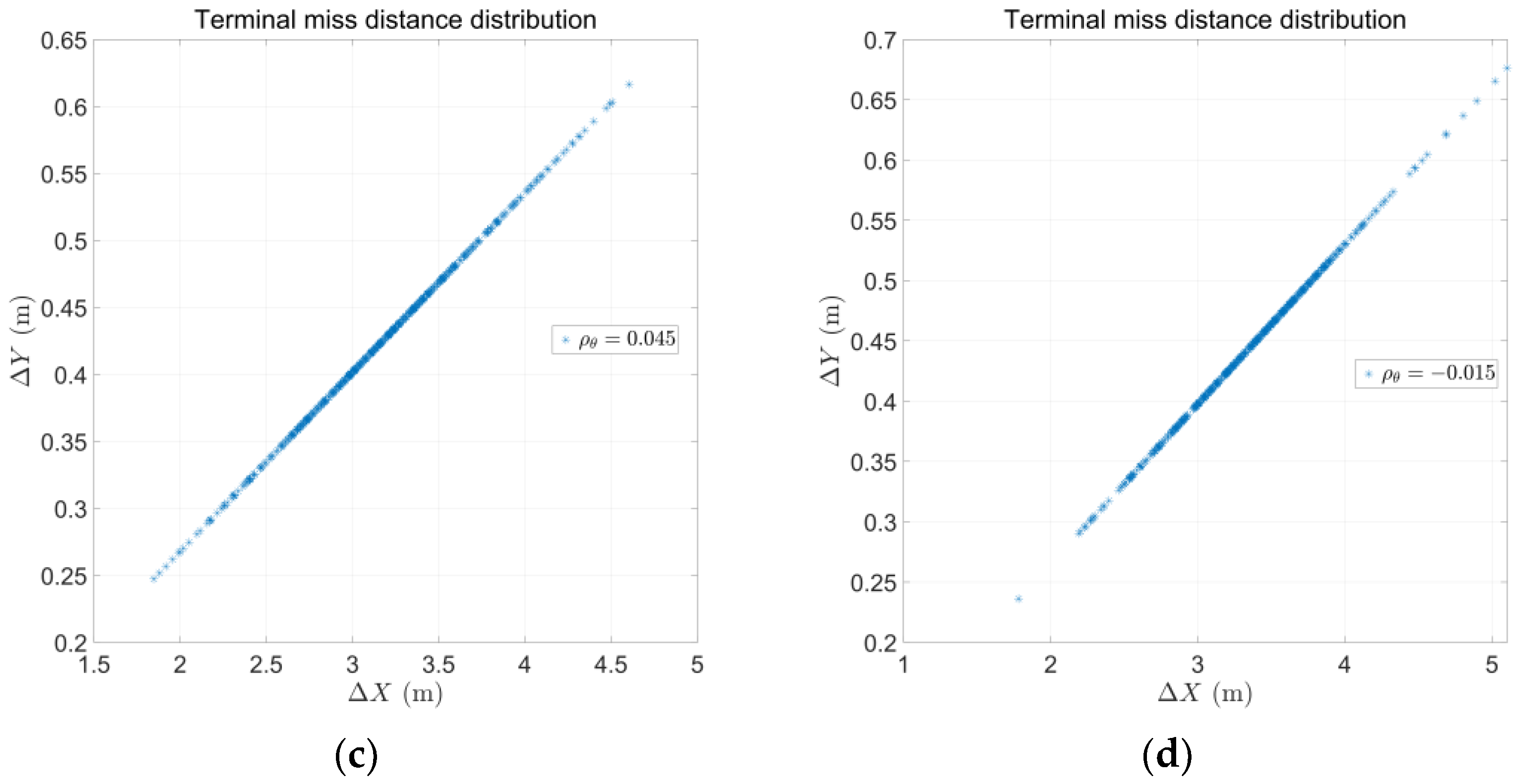
In the end, the terminal miss distance distributions of PNG with LOS angular rate correction are presented in Figure 18a–d, in which the value of the true radome slope varies from −0.015 to 0.045. The simulation results are obtained from 500 Monte-Carlo simulation runs for each case and the miss distance is calculated as follows
Δ X | R ( t f ) cos ( λ ( t f ) ) | Δ Y | R ( t f ) sin ( λ ( t f ) ) |
in which t f = 20   s represents the terminal time. The corresponding statistical results of the terminal miss distance for PNG with LOS angular rate correction are summarized in Table 1, in which the mean values are used for comparison with the miss distance of PNG without correction. From this table, it can be observed that by using LOS angular rate correction, it provides smaller terminal miss distance in different cases; thus, the radome slope estimation and compensation method proposed in this paper provides a promising way to handle the issue of radome refraction for homing guidance.

5. Conclusions

This paper shows that the radome slope can be estimated by using statistical learning techniques along with adaptive filtering methods. The poorly observable issue of estimating the unknown radome slope is overcome by reconstructing the mapping relationship between the look angle and radome error based on the estimated guidance information; thus, the radome slope is estimated by calculating the derivative of the mapping function represented with Gaussian process models. An LOS angular rate corrector is designed by using the estimated radome slope to calibrate the contaminated measurement information due to radome refraction. Simulation results verify that the proposed estimation method can reconstruct the radome slope accurately and improve the guidance performance effectively. Future works include extension of the proposed radome slope estimation method to three-dimensional scenarios, in which collaborative multi-output Gaussian processes will be discussed.

Author Contributions

Writing—original draft, K.L.; formal analysis, B.J.; investigation, K.L., B.J. and N.Z.; writing—review and editing, K.L. and B.J. All authors have read and agreed to the published version of the manuscript.

Funding

This research was funded by the National Natural Science Foundation of China (grant No. 61903084, 61973075, 62073075).

Institutional Review Board Statement

Not applicable.

Informed Consent Statement

Not applicable.

Data Availability Statement

Not applicable.

Conflicts of Interest

The authors declare no conflict of interest.

References

  1. Gong, Z.; Zhou, Z.; Wang, Z.; Lv, Q.; Xu, J.; Jiang, Y. Coordinated Formation Guidance Law for Fixed-Wing UAVs Based on Missile Parallel Approach Method. Aerospace 2022, 9, 272. [Google Scholar] [CrossRef]
  2. Gurfil, P.; Kasdin, J.N. Improving Missile Guidance Performance by In-Flight Two-Step Nonlinear Estimation of Radome Aberration. IEEE Trans. Control Syst. Technol. 2004, 12, 532–541. [Google Scholar] [CrossRef]
  3. Ra, W.; Ahn, S.; Lee, Y.; Whang, I. Time-Varying Radome Slope Estimation for Passive Homing Anti-Ship Missiles. In Proceedings of the IEEE 58th Conference on Decision and Control, Nice, France, 11–13 December 2019; pp. 4940–4945. [Google Scholar]
  4. Seo, M.-G.; Tahk, M.-J. Observability Analysis and Enhancement of Radome Aberration Estimation with Line-of-Sight Angle-Only Measurement. IEEE Trans. Aerosp. Electron. Syst. 2015, 51, 3321–3331. [Google Scholar]
  5. Palumbo, N.F.; Blauwkamp, R.A.; Lloyd, J.M. Basic Principles of Homing Guidance. Johns Hopkins APL Tech. Dig. 2010, 29, 25–41. [Google Scholar]
  6. Han, S.; Ahn, S.; Ra, W.; Park, J.B. Missile Radome Error Compensation using Modified Interacting Multiple Model Kalman Filter. In Proceedings of the 14th International Conference on Control, Automation and Systems, Gyeonggi-do, Korea, 22–25 October 2014; pp. 391–395. [Google Scholar]
  7. Jalali-Naini, S.H. Normalized Miss Distance Analysis of Single-Lag Optimal Guidance Lawwith Radome Effect, Saturation and Fifth-Order Control System. Sci. Iran. 2014, 21, 1683–1692. [Google Scholar]
  8. Zarchan, P. Tactical and Strategic Missile Guidance, 6th ed.; American Institute of Aeronautics and Astronautics, Inc.: Reston, VA, USA, 2012; p. 555. [Google Scholar]
  9. Li, C.; Wang, J.; Huang, P. Optimal Cooperative Line-of-Sight Guidance for Defending a Guided Missile. Aerospace 2022, 9, 232. [Google Scholar] [CrossRef]
  10. Nesline, F.; Zarchan, P. Radome Induced Miss Distance in Aerodynamically Controlled Homing Missiles. In Proceedings of the 17th Fluid Dynamics, Plasma Dynamics and Lasers Conference, Snowmass, CO, USA, 25–27 June 1984; p. 84-1845. [Google Scholar]
  11. Li, B.; Tang, P.; Xu, H.; Zheng, D. Terminal Impact Angle Control Guidance Law Considering Target Observability. Aerospace 2022, 9, 193. [Google Scholar] [CrossRef]
  12. Yueh, W.; Lin, C.-F. Guidance Performance Analysis with In-Flight Radome Error Calibration. J. Guid. Control Dyn. 1985, 8, 666–669. [Google Scholar] [CrossRef]
  13. Klein, I.; Rusnak, I. Loop-Shaping Approach to Mitigate Radome Effects in Homing Missiles. J. Guid. Control Dyn. 2017, 40, 1789–1795. [Google Scholar] [CrossRef]
  14. Deng, Y.; Ren, J.; Wang, X.; Cai, Y. Midcourse Iterative Guidance Method for the Impact Time and Angle Control of Two-Pulse Interceptors. Aerospace 2022, 9, 323. [Google Scholar] [CrossRef]
  15. Bai, R.; Xia, Q.; Du, X. The Study of Guidance Performance of a Phased Array Seeker with Platform. Optik 2017, 132, 9–23. [Google Scholar] [CrossRef]
  16. Zheng, D.; Lin, D.; Wang, J.; Xu, X. Dynamic Stability of Rolling Missiles Employing a Two-Loop Autopilot with Consideration for the Radome Aberration Parasitic Feedback Loop. Aerosp. Sci. Technol. 2017, 61, 1–10. [Google Scholar] [CrossRef]
  17. Nesline, F.W. Missile Guidance for Low-Altitude Air Defense. J. Guid. Control 1979, 2, 283–289. [Google Scholar] [CrossRef]
  18. Lin, S.; Lin, D.; Wang, W. A Novel Online Estimation and Compensation Method for Strapdown Phased Array Seeker Disturbance Rejection Effect Using Extended State Kalman Filter. IEEE Access 2019, 7, 172330–172340. [Google Scholar] [CrossRef]
  19. Das, R. Advances in Active Radar Seeker Technology. Def. Sci. J. 2005, 55, 329. [Google Scholar] [CrossRef] [Green Version]
  20. Tiwari, P.; Vora, P.; Bhattacharjee, R. In Flight Radome Error Compensation through Simulated Test Data. In Proceedings of the AIAA Guidance, Navigation and Control Conference and Exhibit, San Francisco, CA, USA, 15–18 August 2005; p. 6454. [Google Scholar]
  21. Lin, C.-L. Stability Analysis of Radome Error and Calibration Using Neural Networks. IEEE Trans. Aerosp. Electron. Syst. 2001, 37, 1442–1450. [Google Scholar]
  22. Kang, J.; Xiong, Z.; Wang, R.; Zhang, L. Multi-Layer Fault-Tolerant Robust Filter for Integrated Navigation in Launch Inertial Coordinate System. Aerospace 2022, 9, 282. [Google Scholar] [CrossRef]
  23. Paris, D. Computer-Aided Radome Analysis. IEEE Trans. Antennas Propag. 1970, 18, 7–15. [Google Scholar] [CrossRef]
  24. Jeng-Hwa, C.; Kuan-Kin, C. Analysis of A Two-Dimensional Radome of Arbitrarily Curved Surface. IEEE Trans. Antennas Propag. 1990, 38, 1565–1568. [Google Scholar] [CrossRef] [Green Version]
  25. Lee, H.-S.; Park, H. Prediction of Radome Bore-sight Errors using a Projected Image of Source Distributions. Prog. Electromagn. Res. 2009, 92, 181–194. [Google Scholar] [CrossRef] [Green Version]
  26. Asad, M.; Khan, S.; Ihsanullah; Mehmood, Z.; Shi, Y.; Memon, S.A.; Khan, U. A split target detection and tracking algorithm for ballistic missile tracking during the re-entry phase. Def. Technol. 2020, 16, 1142–1150. [Google Scholar] [CrossRef]
  27. Hu, Y.; Gao, C.; Jing, W. Joint State and Parameter Estimation for Hypersonic Glide Vehicles Based on Moving Horizon Estimation via Carleman Linearization. Aerospace 2022, 9, 217. [Google Scholar] [CrossRef]
  28. Zarchan, P.; Gratt, H. Adaptive Radome Compensation using Dither. J. Guid. Control Dyn. 1999, 22, 51–57. [Google Scholar] [CrossRef]
  29. Han, S.S.; Jang, S.K.; Lee, S.J. Radome Compensation using Adaptive Particle Filter. IFAC Proc. Vol. 2007, 40, 43–48. [Google Scholar] [CrossRef]
  30. Yueh, W.R. Adaptive Estimation Scheme for Radome Error Calibration. In Proceedings of the 22nd IEEE Conference on Decision and Control, San Antonio, TX, USA, 14–16 December 1983; pp. 546–551. [Google Scholar]
  31. Lin, J.-M.; Chau, Y.-F. Radome Slope Compensation using Multiple-model Kalman Filters. J. Guid. Control Dyn. 1995, 18, 637–640. [Google Scholar] [CrossRef]
  32. Wang, Y.; Wang, J.; He, S.; Shin, H.-S.; Tsourdos, A. Optimal Guidance with Active Observability Enhancement for Scale Factor Error Estimation of Strapdown Seeker. IEEE Trans. Aerosp. Electron. Syst. 2021, 57, 4347–4362. [Google Scholar] [CrossRef]
  33. Zheng, D.; Lin, D.; Xu, X.; Tian, S. Dynamic Stability of Rolling Missile with Proportional Navigation & PI Autopilot considering Parasitic Radome Loop. Aerosp. Sci. Technol. 2017, 67, 41–48. [Google Scholar]
  34. Süli, E.; Mayers, D.F. An Introduction to Numerical Analysis; Cambridge University Press: Cambridge, UK, 2003. [Google Scholar]
  35. Bar-Shalom, Y.; Li, X.R.; Kirubarajan, T. Estimation with Applications to Tracking and Navigation, Theory, Algorithms and Software; Wiley-Interscience Publication: Hoboken, NJ, USA, 2008. [Google Scholar]
  36. Julier, S.J.; Uhlmann, J.K. Unscented Filtering and Nonlinear Estimation. Proc. IEEE 2004, 92, 401–422. [Google Scholar] [CrossRef] [Green Version]
  37. Williams, C.K.; Rasmussen, C.E. Gaussian Processes for Machine Learning; MIT Press: Cambridge, MA, USA, 2006; Volume 2. [Google Scholar]
  38. Song, T.L.; Lee, D.; Shin, S.J. Active homing performance enhancement with multiple model radome slope estimation. Proc. Inst. Mech. Eng. Part G J. Aerosp. Eng. 2005, 219, 217–224. [Google Scholar] [CrossRef]
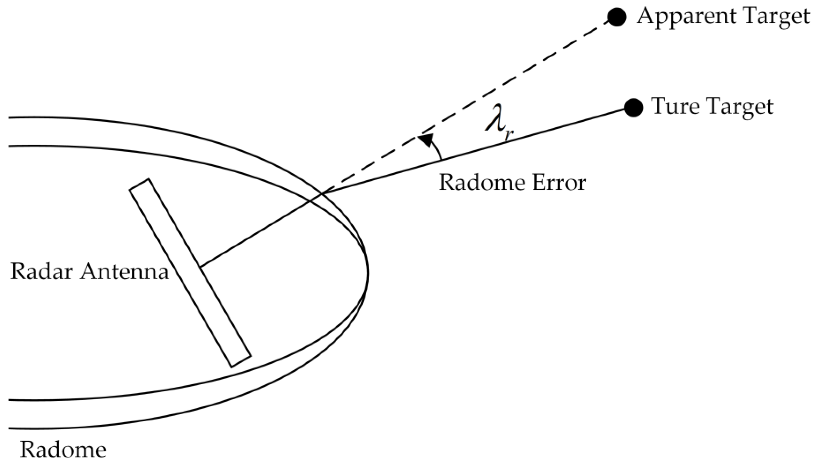
Figure 1. Radome refraction physics.
Aerospace 09 00626 g001
Figure 2. Planar engagement geometry.
Aerospace 09 00626 g002
Figure 3. PN guidance system considering the radome refraction effect.
Aerospace 09 00626 g003
Figure 4. Engagement kinematics between the missile and target.
Aerospace 09 00626 g004
Figure 5. PN guidance system with LOS angular rate corrector.
Aerospace 09 00626 g005
Figure 6. Structure of the IMM estimator.
Aerospace 09 00626 g006
Figure 7. A block diagram of the proposed LOS angular rate corrector.
Aerospace 09 00626 g007
Figure 8. Trajectory of the LOS angle and corresponding estimates.
Aerospace 09 00626 g008
Figure 9. Trajectory of the relative distance and corresponding estimates.
Aerospace 09 00626 g009
Figure 10. Trajectory of the flight path angle and corresponding estimates.
Aerospace 09 00626 g010
Figure 11. Trajectory of the look angle and corresponding estimates.
Aerospace 09 00626 g011
Figure 12. Trajectory of the radome error and corresponding estimates.
Aerospace 09 00626 g012
Figure 13. Estimation of radome slope via extended Kalman filter (EKF), interacting multiple-model (IMM) estimator and the proposed Gaussian process regression (GPR)-based method.
Aerospace 09 00626 g013
Figure 14. Flowchart of the proposed LOS angular rate corrector.
Aerospace 09 00626 g014
Figure 15. Deviation between the contaminated LOS angular rate λ ˙ M E and the true LOS angular rate λ ˙ with different values of the radome slope ρ θ .
Aerospace 09 00626 g015
Figure 16. Estimation error of the radome slope ρ θ in different cases.
Aerospace 09 00626 g016
Figure 17. Deviation between the corrected LOS angular rate λ ˙ c o r r and the true LOS angular rate λ ˙ with different values of the radome slope ρ θ .
Aerospace 09 00626 g017
Figure 18. Terminal miss distance distribution for PNG with LOS angular rate correction. (a) ρ θ   =   0.025 , (b) ρ θ   =   0.035 , (c) ρ θ   =   0.045 , (d) ρ θ   =   0.015 .
Aerospace 09 00626 g018aAerospace 09 00626 g018b
Table 1. Comparison of terminal miss distance for PNG with/without LOS angular rate correction.
Miss Distance (m) ρ θ = 0.015 ρ θ = 0.025 ρ θ = 0.035 ρ θ = 0.045
PNG with correction3.78033.16753.39143.5661
PNG without correction6.87186.12656.42676.7251
Publisher’s Note: MDPI stays neutral with regard to jurisdictional claims in published maps and institutional affiliations.