Abstract
Vertical takeoff and vertical landing (VTVL) vehicles, based on throttling liquid rocket engines, are attracting increasing attention for their validation of guidance and control techniques during landing. However, validation requires the vehicle to fly in a special trajectory with multiple constraints. Propellant consumption should be carefully calculated for the purpose of carrying more experimental devices during the flight, which makes conducting minimum-propellant trajectory optimization a necessity. This study focuses on the optimization of VTVL vehicles based on a throttling liquid rocket engine. Three flight scenarios applicable to this vehicle are proposed, namely, VTVL vehicles without horizontal movement, VTVL vehicles with horizontal movement, and vertical takeoff and autonomous landing with horizontal movement. Trajectory optimization using the Gauss pseudospectral method (GPM) was conducted during the abovementioned flight scenarios. The results show that the GPM provides excellent solutions for trajectory optimization in the different scenarios. In VTVL vehicles with horizontal movement, vertical takeoff, and autonomous landing with horizontal movement scenarios, the thrust appears in a similar bang–bang control. Meanwhile, in VTVL vehicles without a horizontal movement scenario, the thrust appears like a segmented bang–bang control, which we call regulative bang–bang control. Moreover, by introducing the thrust derivative into the optimization objective using a weighted method, thrust fluctuation can be restrained. To ensure the compatibility of switching the flight among the three scenarios, the carried propellant mass should be decided based on the third flight scenario.
1. Introduction
With the rise of the American plan for returning to the moon [1], vertical takeoff and vertical landing (VTVL) [2,3] vehicles, based on throttling liquid rocket engines [4,5], are attracting more and more attention in validating the key techniques for lunar landing. For example, Morpheus and Grasshopper validated many technologies, including the liquid oxygen/liquid methane (LOX/LCH4) propulsion and Autonomous Precision Landing and Hazard Avoidance Technology (ALHAT). To complete validation and consider the applicability of some navigation systems, VTVL vehicles needs to fly in a particular trajectory. Furthermore, trajectory optimization should be developed to make use of limited propellant.
Among the successful VTVL vehicles using a throttling liquid rocket engine, Morpheus [6] completed 14 free flights based on a pressure-feed engine [7] and achieved a 250 m flight altitude with a 406 m flight distance [8,9]. Xombie achieved a 495.6 m flight altitude with an 800 m flight distance. DX-XA, based on the expander cycle engine [10], achieved a 3139.4 m flight altitude with a 106.7 m flight distance. Based on the gas generator engine, Grasshopper, from Space-X, achieved a 744 m flight altitude. For the propulsion of the above vehicles, more propellant is consumed to achieve the same trajectory given the low specific impulse. This may be more serious for a pressure-feed system, given the large system dry mass [11,12]. Therefore, to allow for a larger dry mass and to carry more experimental devices, consuming less propellant in a particular trajectory would be advantageous.
At present, trajectory optimization methods are divided into two major classes known as indirect methods and direct methods [13,14]. The indirect method indirectly optimizes performance index. It has the advantages of high precision and satisfying necessary first-order optimal conditions. Nevertheless, this method has a complex solution process, a small convergent domain, and high requirements for unknown boundary conditions, along with initial guessing of coordination variables [15]. However, the direct method develops fast, given its large convergent domain, and requires no initial guessing of coordination variables [16]. As one of the direct methods, the pseudospectral method [17] has been widely adopted [18] because of its high computation efficiency [19] and ability for attaining real-time optimal trajectory [20]. The pseudospectral method includes the Chebyshev pseudospectral method (CPM), the Legendre pseudospectral method (LPM) [21], the Gauss pseudospectral method (GPM), and the Radau pseudospectral method (RPM). Compared with other pseudospectral methods, GPM [22] can achieve higher precision based on less nodes. Moreover, the Karush–Kuhn–Tucker (KKT) condition for the non-linear programming (NLP) problem discretized by this method is equivalent to the first-order optimal condition for the discrete Hamiltonian boundary value problem [23]. GPM has been widely used in hypersonic vehicle trajectory optimization and guidance [24], solid booster ascent [25], helicopter trajectory planning [23], unmanned aerial vehicle (UAV) trajectory planning [26], manned lunar landing orbit optimization [15], chaotic system control [16], and space debris removal using tethered systems [27,28].
Therefore, GPM has been used to optimize the trajectory of VTVL vehicles powered by throttling liquid rocket engines. Having regard to existing vehicle trajectories, and in light of difficult degrees along with verification purposes, three flight scenarios have been proposed in this study, namely, VTVL vehicles without horizontal movement, VTVL vehicles with horizontal movement, and vertical takeoff and autonomous landing with horizontal movement. These flight scenarios have been optimized to minimize propellant consumption and thrust fluctuation. The results show that GPM is applicable to optimizing these flight scenarios in VTVL vehicles.
2. Multi-Scenario Overview
The three flight scenarios proposed in this study are mainly used for VTVL vehicles powered by throttling liquid rocket engines. This vehicle is flat in structure, with four axisymmetric propellant tanks and an irregular aerodynamic shape. The specific layout can be referred to as NASA’s Morpheus vehicle. These characteristics show that this vehicle is more suitable for low-speed situations.
The engine system control corresponding to the different flight scenarios changes from easy to difficult, and verified key technologies are gradually deepened. In general, the first flight scenario is used to verify variable thrust technology, the second flight scenario is used to verify deep throttling technology, thrust vector control technology, navigation guidance and control technology, and the third flight scenario focuses on the verification of autonomous landing and risk avoidance technology. These three flight scenarios will be described in detail below.
2.1. VTVL Vehicles without Horizontal Movement: First Flight Scenario
In the first scenario, the vehicle takes off vertically, and descends vertically after reaching the target altitude. Throughout the process, the engine does not swing. The purpose of the first scenario is to validate throttling engine performance. A flight sketch of the first scenario is shown in Figure 1. The design parameters are given in Table 1. In the first scenario, the influences of cross wind and other disturbances are ignored.
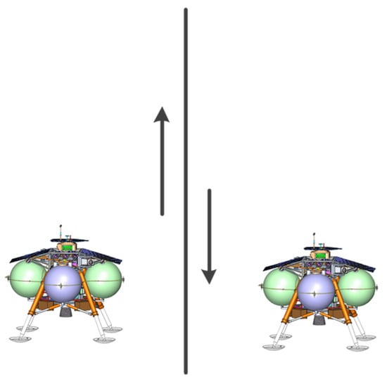
Figure 1.
First flight scenario sketch.

Table 1.
Design input for the first scenario.
2.2. VTVL Vehicles with Horizontal Movement: Second Flight Scenario
In the second scenario, the vehicle takes off vertically to the target altitude, then descends while translating. When it reaches the target distance, it lands vertically at the target point. During the vertical ascent and descent, the engine does not swing. However, during the translation process, the engine first swings forward 5° to accelerate the vehicle, then reverse swings 5° to slow down the vehicle. When the vehicle reaches the target distance, the engine remains vertical. The purpose of the second scenario is to validate the GNC system. A sketch of the second flight scenario is shown in Figure 2. Table 2 shows the design parameters of the second scenario. Compared with the first scenario, the maximum altitude is lower given translation.
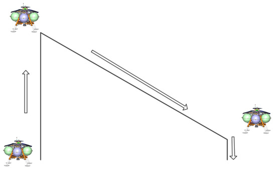
Figure 2.
Second flight scenario sketch.
Table 2.
Design input for the second scenario.
2.3. Vertical Takeoff and Autonomous Landing with Horizontal Movement: Third Flight Scenario
In the third scenario, the vehicle first takes off vertically, then translates after reaching the maximum altitude. Once the vehicle reaches the target distance, it descends vertically. When descending to a certain altitude, the vehicle commences autonomous landing, and chooses the landing site autonomously according to the topographic situation around the target position. During the whole flight process, the engine condition is consistent with that of the second scenario before the autonomous landing phase. However, in the autonomous landing phase, the engine can swing 5° positively and negatively. The purpose of the third scenario is to validate ALHAT. A sketch of the third flight scenario is given in Figure 3. The design parameters, including two cases, are shown in Table 3.
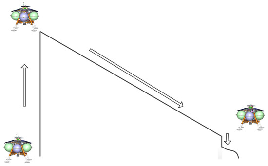
Figure 3.
Third flight scenario sketch.
Table 3.
Design input for the third scenario.
3. Dynamic Model
The influence of aerodynamics and disturbances is ignored given the small flight altitude and distance. Moreover, the trajectory is two-dimensional in this study. Modeling the vehicle can be attained by the following dynamic equations:
where x is the translation distance, m; vx is the translation velocity, m/s; m is the vehicle mass, kg; y is the vertical distance, m; vy is the vertical velocity, m/s; F is the engine thrust, N; α is the nozzle angle relative to the vertical direction. α is 5° at acceleration, −5° at deceleration, and 0° in vertical flight. Isp is the engine specific impulse decided by the engine chamber pressure, the mixture ratio, and the nozzle area ratio, m/s. g is the gravity acceleration, m/s2.
The above dynamic equations can be expressed as a non-linear model:
where is the state variable and u = is the control variable.
4. Trajectory Optimization Method Based on the Gauss Pseudospectral Method
4.1. Problem Formulation
The purpose of VTVL vehicle trajectory optimization is to provide a theoretical optimum trajectory for demonstration and verification. Therefore, this problem can be described as the design of u to minimize propellant consumption. As large thrust fluctuation may lead to abnormal work conditions of the throttling engine, minimizing thrust fluctuation is set as the other optimization objective. To minimize thrust fluctuation is to minimize the 2-norm of the thrust change rate.
In the meantime, F should satisfy Equation (2) and the following constraints, including the terminal constraint, the state constraint, and the control constraint:
For the different flight scenarios, the above constraints are different. The terminal constraint is determined by design input, wherein the speed of the vehicle during soft landing is less than 2 m/s [29,30]. For the state constraint, the position is determined by design input. Assume that the given speed is the maximum value without considering interference. The upper limit of the vehicle mass constraint is determined by the design input, and its lower limit is a small value considering a long flight time, which can be adjusted when the optimization result is unsatisfactory. The thrust throttling ratio is considered to be 5:1. For the control constraint, the thrust change rate does not exceed 1/4 of the maximum thrust and can be adjusted when the optimization result is unsatisfactory. For the first flight scenario, the terminal constraint, the state constraint, and the control constraint are:
For the second scenario, the terminal constraint, the state constraint, and the control constraint are:
For two cases of the third scenario, the terminal constraint, the state constraint, and the control constraint are:
4.2. Gauss Pseudospectral Method
The Gauss pseudospectral method essentially discretizes the state and control variables at the Gauss points and constructs the Lagrange interpolation polynomials with discrete points as nodes to approximate the state and control variables. Further, by deriving the global interpolation polynomials to approximate the state variable derivatives, differential equation constraints are transformed into algebraic constraints. Finally, vehicle trajectory optimization is converted to a NLP problem [31]. Generally, GPM solves the NLP problem by sequential quadratic programming (SQP) [16,25]. SQP [32,33,34] is considered to be one of the most effective methods for solving NLP problems because of its global convergence and superlinear local convergence [35]. The SQP includes five basic steps, namely, time domain transformation, discretization of state and control variables, differential equation transformation, performance index transformation, and terminal constraint transformation. The specific method can be found in the literature [24].
In this study, the optimization control variable is obtained by the Gauss pseudospectral method and brought into the original dynamic equations. Then, the optimization trajectory is compared with the calculation trajectory by the above original equations to verify the reliability of the optimized solution. The optimality of the results can indirectly be judged by the Hamiltonian function. The Hamiltonian function is a function of the state variable, control variable, costate variable and KKT multiplier vector. According to the optimal control theory, when the control quantity has no boundary and the Hamiltonian function does not contain time explicitly, if the optimization result is the optimal solution, the Hamiltonian function remains constant.
4.3. Multi-Objective Processing
This study contains two optimization objectives: minimizing propellant consumption and thrust fluctuation. Since minimizing propellant consumption is the main optimization objective, thrust fluctuation is kept as small as possible on this basis. Therefore, the weighted method is used to deal with this problem, namely, multiplying a weighted coefficient by the second optimization objective:
where the weighted coefficients for different scenarios are different, as shown in Table 4.
Table 4.
Weighted coefficients for different scenarios.
5. Numerical Simulation Results and Discussions
5.1. Simulation Results for the First Scenario
Figure 4 shows the variation of flight altitude in the first scenario with time. From the comparison, the optimization results are in good agreement with the calculation results, and the landing error is only 0.006 m, which shows successful optimization. At the same time, the fluctuation range of the Hamilton function is less than 0.7, which proves the optimality.
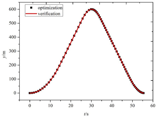
Figure 4.
Flight height in the first scenario vs. time.
Figure 5 and Figure 6 show the optimization speed and acceleration curves in the first scenario, respectively. First, due to the maximum speed limitation, uniform speed occurs in both rising and falling stages after reaching the maximum speed. Second, due to the maximum speed limitation, there are two steps in acceleration, namely, one lower step and one upper step.
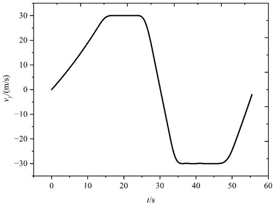
Figure 5.
Vertical velocity for the first scenario vs. time.
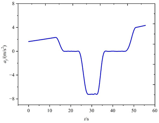
Figure 6.
Vertical acceleration in the first scenario vs. time.
Figure 7 shows thrust variation versus time in the first scenario. It can be seen that under given constraints, the thrust presents the process of a lower step, cavity, and upper step to achieve the optimization objective. These steps are caused by the velocity constraint. The thrust always keeps to a maximum in the step’s initial ascending and ultimate descending stages to obtain upward maximum acceleration, which consumes less propellant. In the step’s ascending end and descending starting stages, the thrust is kept to a minimum to obtain maximum downward acceleration. In other words, except for the two steps, the thrust switches between the maximum and minimum values, similar to a segmented bang–bang control [36], which may be called regulative bang–bang control.
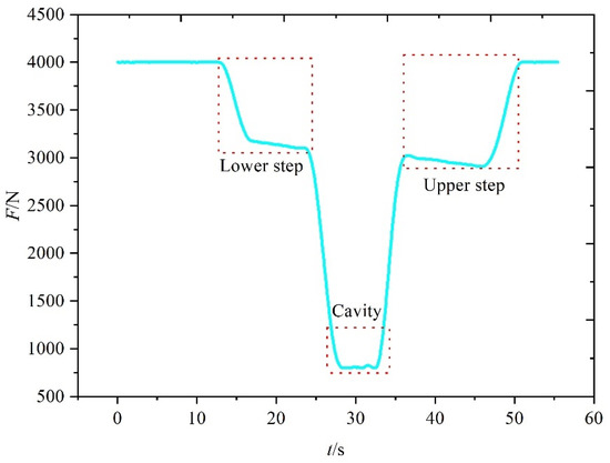
Figure 7.
Thrust in the first scenario vs. time.
Figure 8 shows the propellant mass flow rates and the vehicle mass variation with time in the first scenario. Assuming that the mixing ratio is constant, and the change of ground specific impulse is small due to low flight altitude, the change curve of the oxidants and fuel can be obtained according to the thrust curve, which has the same change trend as the thrust curve. It can be seen that the mass of the aircraft changes slowly when the propellant flow is at the bottom of the cavity. During the whole process, the propellant flow has both a large slope linear change and a small slope linear change. By optimization, the propellant consumption can be reduced by about 40% to achieve the same flight altitude (referring to the lunar module descent engine). Based on satisfying the flight altitude, the combination of the step and slope is adopted to obtain the unoptimized thrust curve, as shown in Equation (10). By solving Equation (1) considering this unoptimized curve, unoptimized results can be obtained. The reason is that the vehicle always needs to overcome gravity to work. Through optimization, the shorter the flight time, the less the propellant that is consumed to overcome gravity.
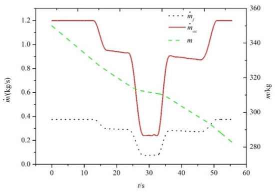
Figure 8.
Propellant mass flow rates and vehicle mass in the first scenario vs. time.
5.2. Simulation Results for the Second Scenario
Figure 9 shows the comparison between the optimization result and the calculation result in the second scenario. First, these two results are in good agreement. Second, the vehicle appears to rise during the translation process, because the thrust may be greater than gravity to obtain a larger horizontal acceleration. At the same time, the fluctuation range of the Hamilton function is less than 0.13, which proves the optimality.
Figure 9.
Flight trajectory in the second scenario.
Figure 10 shows the vehicle mass variation with time in the second scenario. It can be seen that 80.2 kg of propellant is consumed during the entire flight. Moreover, at each transition between the adjacent stages, the vehicle mass changes slowly because of the low thrust near the transition point and the small propellant flow rate.
Figure 10.
Vehicle mass in the second scenario vs. time.
Figure 11 shows the second scenario thrust variation with time. The whole flight process includes the ascent, the acceleration translation, the deceleration translation, and the descent. In general, during the deceleration translation, the thrust fluctuates slightly. However, due to the small fluctuation, the influence on the throttling engine is negligible. The ascent is the same as that in the first scenario. During the acceleration and deceleration translations, the maximum thrust runs some time to obtain a large lateral acceleration. In the translation, a thrust cavity, namely, a minimum thrust stage, also occurs to obtain a large vertical acceleration. Because of the contradiction between the large lateral acceleration and the downward vertical acceleration, a situation arises whereby the thrust alters between the maximum and minimum values in the translation. Overall, after the ascent the thrust basically switches between the maximum and minimum values, which is similar to the bang–bang control. Therefore, for the second scenario, the thrust represents a combination between the regulative bang–bang control and the similar bang–bang control.
Figure 11.
Thrust in the second scenario vs. time.
Figure 12 shows the propellant mass flow rates and the vehicle mass variation with time in the first scenario. At the transition of each of the two stages, the vehicle mass changes slowly because the thrust near the transition point is at a low level and the propellant mass flow rates are small.
Figure 12.
Propellant mass flow rates and vehicle mass in the second scenario vs. time.
5.3. Simulation Results for the Third Scenario
5.3.1. Results under Case 1 in the Third Scenario
Figure 13 shows the flight trajectory under case 1 in the third scenario. It can be seen that there is an error between the optimization result and the calculation result, especially near the target point. At the same time, the fluctuation range of the Hamilton function is less than 0.12, which proves the optimality. Figure 14 shows the vehicle mass variation against time. A total of 84.3 kg of propellant is consumed during the entire flight.
Figure 13.
Flight trajectory under case 1 in the third scenario.
Figure 14.
Vehicle mass under case 1 in the third scenario vs. time.
Figure 15 shows thrust variation with time under case 1 in the third scenario. It can be seen that before autonomous landing, the thrust variation trend is consistent with that in the second scenario. However, the thrust fluctuation is more obvious, indicating that the applicability of the optimization method becomes worse with working condition complexity. In autonomous landing, the thrust presents an oblique N type. Since the autonomous landing altitude and distance are uncertain, the thrust variation of the autonomous landing stage is random.
Figure 15.
Thrust under case 1 in the third scenario vs. time.
Figure 16 shows the propellant mass flow rates and the vehicle mass variation with time under case 1 in the third scenario. Compared with the second scenario, the fluctuation of the propellant mass flow rates increases and the requirement for the variable thrust engines is higher. Therefore, it is considered that there are some limitations in eliminating the fluctuation for the weighted method. In addition, due to the existence of autonomous landing in the third scenario, the variation of the propellant mass flow rates does not show a certain regularity.
Figure 16.
Propellant mass flow rates and vehicle mass under case 1 in the third scenario vs. time.
5.3.2. Results under Case 2 in the Third Scenario
Figure 17 shows the flight trajectory under case 2 in the third scenario. Compared with case 1, the deviation between the optimization result and the calculation result is smaller. At the same time, the fluctuation range of the Hamilton function is less than 0.09, which proves the optimality. Figure 18 shows the vehicle mass variation with time under case 2 in the third scenario. A total of 85.7 kg of propellant is consumed during the entire flight. Compared with case 1, more propellant is consumed in case 2.
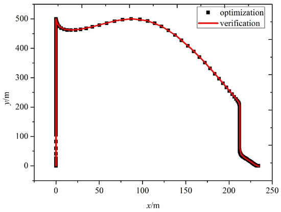
Figure 17.
Flight trajectory under case 2 in the third scenario.
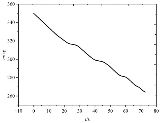
Figure 18.
Vehicle mass under case 2 in the third scenario vs. time.
Figure 19 shows the thrust variation with time under case 2 in the third scenario. It can be seen that a somewhat large fluctuation occurs in the acceleration translation. In general, as seen in two cases in the third scenario, the thrust does not express the similar bang–bang control type in autonomous landing because of the small flight distance and greater constraints.
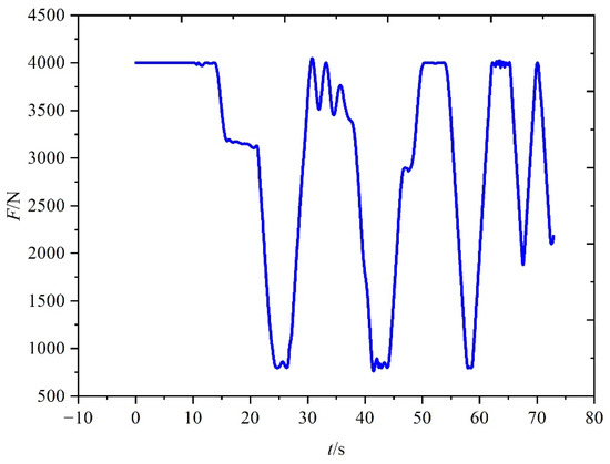
Figure 19.
Thrust under case 2 in the third scenario vs. time.
Figure 20 shows the propellant mass flow rates and the vehicle mass variation with time under case 2 in the third scenario. Compared with case 1 in the third scenario, the fluctuation of the propellant mass flow rates is reduced, and there is a relatively violent fluctuation in the accelerated translation stage. Further, it shows that for complex conditions, the weight method has some limitations in removing fluctuations.
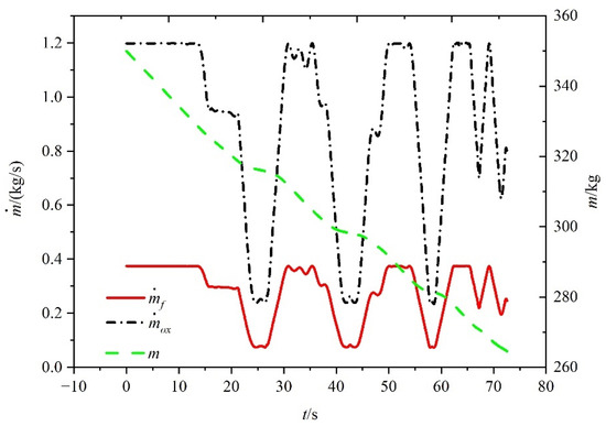
Figure 20.
Propellant mass flow rates and vehicle mass under case 2 in the third scenario vs. time.
5.4. Comparison among Three Scenarios
Considering the compatibility of the three flight scenarios, the consumed propellant mass should be determined by the third scenario. Moreover, it is appropriate to carry 85.7 kg of propellant according to case 2 in the third scenario, as shown in Table 5, because the vehicle should have the ability to select the landing point independently around the target point.
Table 5.
Comparison of results for the three flight scenarios.
6. Conclusions
In this study, three typical flight scenarios were proposed based on ground vertical takeoff and vertical landing vehicles powered by a throttling thrust rocket engine, including VTVL vehicles without horizontal movement, VTVL vehicles with horizontal movement, and vertical takeoff and autonomous landing with horizontal movement. Moreover, the Gauss pseudospectral method was used to develop trajectory optimization for the above flight scenarios.
Simulation results show that, on the one hand, the Gauss pseudospectral method is suitable for trajectory optimization of ground vertical takeoff and vertical landing vehicles. In the optimization process, reducing the propellant consumption as much as possible can increase the space left for the vehicle’s structure quality. Moreover, the thrust is in the form of regulative bang–bang control in the first scenario. However, the thrust expresses the form of similar bang–bang control in the translation and vertical landing process of the second and third scenarios. On the other hand, by introducing the two-norm term of the thrust variation rate into the optimization objective through the weighted method, thrust fluctuation can be effectively suppressed, especially in VTVL vehicles without horizontal movement, in which thrust fluctuation is basically eliminated. Although thrust fluctuations may increase with complex flight scenarios, these fluctuations are within the acceptable range of the throttling thrust rocket engine. In the meantime, to satisfy the multi-scenario compatibility of VTVL vehicles, the carried propellant mass should be greater than that under case 2 in the third scenario.
Author Contributions
Conceptualization, P.C.; Formal analysis, D.Z.; Funding acquisition, P.C.; Investigation, Y.L.; Methodology, Q.H. and P.C.; Validation, C.L. and X.Z.; Visualization, C.L. and Q.H.; Writing–original draft, Y.L.; Writing–review & editing, X.Z. and D.Z. All authors have read and agreed to the published version of the manuscript.
Funding
This research was funded by the National Basic Research Program of China (Grant No. 613239).
Data Availability Statement
Not applicable.
Acknowledgments
The authors would like to express their sincere thanks for the support of the thorough examination of grammar mistakes in paper writing by Jing Chen and Jie Song.
Conflicts of Interest
The authors declare no conflict of interest.
References
- Smith, T.D.; Klem, M.D.; Fisher, K.L. Propulsion Risk Reduction Activities for Nontoxic Cryogenic Propulsion. In Proceedings of the Space 2010 Conference and Exposition, Anaheim, CA, USA, 30 August–2 September 2010. [Google Scholar]
- Zhang, L.; Wei, C.; Wu, R.; Cui, N. Adaptive Fault-Tolerant Control for a Vtvl Reusable Launch Vehicle. Acta Astronaut. 2019, 159, 362–370. [Google Scholar] [CrossRef]
- Ma, L.; Wang, K.; Xu, Z.; Shao, Z.; Song, Z.; Biegler, L.T. Trajectory Optimization for Lunar Rover Performing Vertical Takeoff Vertical Landing Maneuvers in the Presence of Terrain. Acta Astronaut. 2018, 146, 289–299. [Google Scholar] [CrossRef]
- Casiano, M.J.; Hulka, J.R.; Yang, V. Liquid-Propellant Rocket Engine Throttling: A Comprehensive Review. J. Propuls. Power 2010, 26, 897–923. [Google Scholar] [CrossRef]
- Yue, C.; Li, J.; Hou, X.; Feng, X.; Yang, S. Summarization on Variable Liquid Thrust Rocket Engines. Sci. China Ser. E Technol. Sci. 2009, 52, 2918–2923. [Google Scholar] [CrossRef]
- Hurlbert, E.; McManamen, J.; Studak, J. Advanced Development of a Compact 5-15 Lbf Lox/Methane Thruster for an Integrated Reaction Control and Main Engine Propulsion System. In Proceedings of the 47th AIAA/ASME/SAE/ASEE Joint Propulsion Conference & Exhibit, San Diego, CA, USA, 31 July–3 August 2011; American Institute of Aeronautics and Astronautics: Reston, VI, USA, 2011. [Google Scholar]
- Melcher, J.C.; Morehead, R.L. Combustion Stability Characteristics of the Project Morpheus Liquid Oxygen/Liquid Methane Main Engine. In Proceedings of the 50th AIAA/ASME/SAE/ASEE Joint Propulsion Conference, Cleveland, OH, USA, 28–30 July 2014; American Institute of Aeronautics and Astronautics: Reston, VI, USA, 2014. [Google Scholar]
- Crain, T.; Bishop, R.H.; Carson, J.M.; Trawny, N.; Sullivan, J.; Christian, J.A.; Kyle, J.D.; Joel, G.; Chad, H. Approach-Phase Precision Landing with Hazard Relative Navigation: Terrestrial Test Campaign Results of the Morpheus/Alhat Project. In Proceedings of the AIAA Guidance, Navigation, and Control Conference, San Diego, CA, USA, 4–8 January 2016; American Institute of Aeronautics and Astronautics: Reston, VI, USA, 2016. [Google Scholar]
- Carson, J.M.; Robertson, E.; Trawny, N.; Amzajerdian, F. Flight Testing Alhat Precision Landing Technologies Integrated Onboard the Morpheus Rocket Vehicle. In Proceedings of the AIAA SPACE 2015 Conference and Exposition, Pasadena, CA, USA, 31 August–2 September 2015; American Institute of Aeronautics and Astronautics: Reston, VI, USA, 2015. [Google Scholar]
- Marc, W. Rl10a-5—An Assessment of Reusability Demonstrated During the Ssrt Program. In Proceedings of the 32nd Joint Propulsion Conference and Exhibit, Buena Vista, FL, USA, 1–3 July 1996; American Institute of Aeronautics and Astronautics: Reston, VI, USA, 1996. [Google Scholar]
- Pavlov Rachov, P.A.; Tacca, H.; Lentini, D. Electric Feed Systems for Liquid Propellant Rockets. J. Propuls. Power 2013, 29, 1171–1180. [Google Scholar] [CrossRef]
- Soldà, N.; Lentini, D. Opportunities for a Liquid Rocket Feed System Based on Electric Pumps. J. Propuls. Power 2008, 24, 1340–1346. [Google Scholar] [CrossRef]
- Song, Y.; Gong, S. Solar Sail Trajectory Optimization of Multi-Asteroid Rendezvous Mission. Acta Astronaut. 2019, 157, 111–122. [Google Scholar] [CrossRef]
- Betts, J.T. Survey Numerical Methods for Trajectory Optimization. J. Guid. Control. Dyn. 1998, 21, 193–207. [Google Scholar] [CrossRef]
- Peng, Q.; Shen, H.; Li, H. Free Return Orbit Design and Characteristics Analysis for Manned Lunar Mission. Sci. China Technol. Sci. 2011, 54, 3243–3250. [Google Scholar]
- Cao, X. Optimal Control for a Chaotic System by Means of Gauss Pseudospectral Method. Acta Phys. Sin. 2013, 62, 71–78. (In Chinese) [Google Scholar]
- Zhu, Y.W.; Cai, W.W.; Yang, L.P.; Huang, H. Flatness-Based Trajectory Planning for Electromagnetic Spacecraft Proximity Operations in Elliptical Orbits. Acta Astronaut. 2018, 152, 342–351. [Google Scholar] [CrossRef]
- Benson, D.A.; Huntington, G.T.; Thorvaldsen, T.P.; Rao, A.V. Direct Trajectory Optimization and Costate Estimation via an Orthogonal Collocation Method. J. Guid. Control. Dyn. 2006, 29, 1435–1439. [Google Scholar] [CrossRef]
- Jiang, X.; Li, S.; Furfaro, R. Integrated Guidance for Mars Entry and Powered Descent Using Reinforcement Learning and Pseudospectral Method. Acta Astronaut. 2018, 163, 114–129. [Google Scholar] [CrossRef]
- Ross, I.M.; Sekhavat, P.; Fleming, A.; Qi, G. Optimal Feedback Control: Foundations, Examples, and Experimental Results for a New Approach. J. Guid. Control. Dyn. 2008, 31, 307–321. [Google Scholar] [CrossRef]
- Fahroo, F.; Ross, I.M. Advances in Pseudospectral Methods for Optimal Control. In Proceedings of the AIAA Guidance, Navigation and Control Conference and Exhibit, Honolulu, HI, USA, 18–21 August 2008. [Google Scholar]
- Zhang, J.; Chu, X.; Zhang, Y.; Hu, Q.; Zhai, G.; Li, Y. Safe-Trajectory Optimization and Tracking Control in Ultra-Close Proximity to a Failed Satellite. Acta Astronaut. 2018, 144, 339–352. [Google Scholar] [CrossRef]
- Meng, S.; Xiang, J.; Luo, Z.; Ren, Y. Optimal Trajectory Planning for Small-Scale Unmanned Helicopter Obstacle Avoidance. J. Beijing Univ. Aeronaut. Astronaut. 2014, 40, 246–251. (In Chinese) [Google Scholar]
- Zhong, W.; Qu, Q.; Yuan, J.; Wu, W. Research on Reentry Integrated Guidance Law of Hypersonic Velocity Aircraft Based on the Gauss Pseudo-Spectral Method. Comput. Meas. Control. 2017, 25, 106–109+113. (In Chinese) [Google Scholar]
- Yang, X.; Zhang, W. Rapid Optimization of Ascent Trajectory for Solid Launch Vehicles Based on Gauss Pseudospectral Method. J. Astronaut. 2011, 32, 15–21. (In Chinese) [Google Scholar]
- Gao, X.Z.; Hou, Z.X.; Guo, Z.; Wang, P.; Zhang, J.T. Research on Characteristics of Gravitational Gliding for High-Altitude Solar-Powered Unmanned Aerial Vehicles. Proc. Inst. Mech. Eng. Part G J. Aerosp. Eng. 2013, 227, 1911–1923. [Google Scholar] [CrossRef]
- Chu, Z.; Wei, T.; Shen, T.; Di, J.; Cui, J.; Sun, J. Optimal Commands Based Multi-Stage Drag De-Orbit Design for a Tethered System During Large Space Debris Removal. Acta Astronaut. 2019, 163, 238–249. [Google Scholar] [CrossRef]
- Chu, Z.; Di, J.; Cui, J. Hybrid Tension Control Method for Tethered Satellite Systems During Large Tumbling Space Debris Removal. Acta Astronaut. 2018, 152, 611–623. [Google Scholar]
- Luo, J.; Wang, M.; Yuan, J. Rapid Lunar Soft-Landing Trajectory Optimization by a Legendre Pseudospectral Method. In Proceedings of the 57th International Astronautical Congress, Valenica, Spain, 2–6 October 2006. [Google Scholar]
- Sostaric, R.; Rea, J. Powered Descent Guidance Methods for the Moon and Mars. In Proceedings of the AIAA Guidance Navigation, and Control Conference and Exhibit, San Francisco, CA, USA, 15–18 August 2005. [Google Scholar]
- Tang, X. Numerical Solution of Optimal Control Problems Using Multiple-Interval Integral Gegenbauer Pseudospectral Methods. Acta Astronaut. 2016, 121, 63–75. [Google Scholar]
- Zhao, W.; Wang, L.; Yin, Y.; Wang, B.; Tang, Y. Sequential Quadratic Programming Enhanced Backtracking Search Algorithm. Front. Comput. Sci. 2018, 12, 316–330. [Google Scholar] [CrossRef]
- Curtis, F.E.; Han, Z.; Robinson, D.P. A Globally Convergent Primal-Dual Active-Set Framework for Large-Scale Convex Quadratic Optimization. Comput. Optim. Appl. 2015, 60, 311–341. [Google Scholar] [CrossRef]
- Gould, N.I.M.; Robinson, D.P. A Second Derivative Sqp Method: Global Convergence. SIAM J. Optim. 2010, 20, 2023–2048. [Google Scholar] [CrossRef]
- Gill, P.E.; Murray, W.; Saunders, M.A. Snopt: An Sqp Algorithm for Large-Scale Constrained Optimization. Siam Rev. 2005, 47, 99–131. [Google Scholar] [CrossRef]
- Zhong, Y. Optimal Control; Tsinghua University Press: Beijing, China, 2015. (In Chinese) [Google Scholar]


Publisher’s Note: MDPI stays neutral with regard to jurisdictional claims in published maps and institutional affiliations. |
© 2022 by the authors. Licensee MDPI, Basel, Switzerland. This article is an open access article distributed under the terms and conditions of the Creative Commons Attribution (CC BY) license (https://creativecommons.org/licenses/by/4.0/).