Roughness Effect on the Flow Past Axisymmetric Bodies at High Incidence

Abstract

The flow at low Mach numbers and high angles of attack over axisymmetric configurations is not symmetric. The mechanism that triggers the asymmetry is a combination of a global (temporal) instability and a convective (spatial) instability. This latter instability is caused by roughness and other geometrical imperfections, which lead to roll angle dependent forces. The flow at these conditions has a complex vortex sheet structure, with two or three different flow regions. An accurate simulation by means of Computational Flow Dynamics (CFD) is thus very challenging, and many researchers have therefore employed Large Eddy Simulation (LES) codes. This study demonstrates that Unsteady Reynolds Averaged Navier-Stokes (URANS) methods are a suitable alternative, if Scale Adaptive Simulation (SAS) is used. This method is capable of capturing the main flow features, provided that fine meshes, which achieve geometrical similarity between the meshed geometry and the real object, and small-time steps are used. It is also demonstrated that, by using URANS methods in combination with SAS, strong differences in the global and local forces depending on the surface roughness of the model are obtained, a result which coincides with several wind tunnel tests.

1. Introduction

This paper contains results shown in a conference paper, presented at the 9th European Conference for Aeronautics and Space Sciences (EUCASS) celebrated in Lille, France, from 28 June–1 July 2022 [1].

The flow field past an axisymmetric body flying at a high angle of attack and low Mach numbers entails large areas of boundary layer separation, and a complex vortex sheet structure. At low angles of attack, the dominant axial flow component keeps the flow attached to the body, developing a normal force, which increases linearly with the angle of attack. At intermediate angles, the increasing adverse pressure gradients on the body surface force the leeside boundary layer to separate, yielding a steady symmetric vortex pair. The normal force then evolves in a nonlinear manner, but there is still no side force. At larger angles of attack the vortices become asymmetric, leading to the appearance of a side force, and a complex unsteady flow pattern at the rear body. At very large angles the axial flow component has little influence and the boundary layer is shed in an unsteady fashion, similar to the wake behind a two-dimensional cylinder normal to the flow, the average side force decaying to zero [2].

There are two dimensionless parameters of the flow domain that affect this basic flow structure: Mach number and Reynolds number. Regarding the Mach number, the asymmetry of the flow disappears as the Mach number increases. The appearance of shocks at the leeward side makes the flow symmetric [2]. Concerning Reynolds number effects, it has been demonstrated in several experimental tests that maximum side forces occur both at laminar and turbulent flow conditions. This behavior reinforces the idea that a global instability of inviscid nature is the origin of the asymmetry [2]. Experiments conducted by Lamont [3] showed this effect; the side forces reduce in the critical Reynolds number region.

Some geometric characteristics are relevant for the flow structure: nose angle, bluntness, fineness ratio and roughness. Keener and Chapman [4] introduced the idea of a hydrodynamic (inviscid) mechanism as the origin of the asymmetry. The asymmetric wake is the result of an inviscid instability that occurs when two vortices are “crowded together” near the tip of the body. One vortex moves away from the body and the other moves underneath the first. Champigny [2] showed that above a certain angle of attack, very small perturbations (inhomogeneity in the main flow, surface irregularities, geometrical defects, etc.) are sufficient to cause the vortex system to go from an unstable symmetric state to a stable asymmetric structure. Different experimental tests for ogives or cones have shown an empirical correlation between the angle of attack for onset of asymmetry and the semi apex angle ${\delta }_n$, such that: ${\alpha }_{onset}=2\cdot {\delta }_n$ [5]. This value is reduced as the fineness ratio increases [2], indicating an additional instability due to the afterbody. Accordingly, bluntness delays substantially the onset for asymmetry and reduces the side force significantly [5].

Roughness, or small eccentricities or other geometrical body imperfections, are relevant factors in the appearance of asymmetric flow patterns. At a certain angle of attack, experiments have shown that the side forces depend on the roll angle [2,5,6,7,8,9]. This is the azimuth angle at each cross section, measured from the leeside clockwise. Two different series of experiments, one described by P. Champigny on an ogive cylinder configuration [2,7] and another conducted by Mahadevan et al. on a cone configuration [8], reported roll angle dependent side forces, due to the roughness of the model. The results for the ogive cylinder showed a bi-stable behavior for smooth surfaces, while for a rough surface the side force depended on the roll angle, leading to large variations of the side force magnitude. Similarly, the results of the rough surface model of a cone [8] showed a sinusoidal variation of the side force with the roll angle, while there was a bi-stable pattern of the side force –either negative or positive of similar magnitude- at the range of moderate to high angles of attack for the smooth surface model.

Experiments conducted by Kruse, Keener and Chapman [6] showed that rotating the tip of an axisymmetric body has large effects on the side forces; the rotation of the afterbody (cylindrical part) holding the tip had also a large effect. Then, minor surface irregularities may activate a convective instability, also in zones far from the tip. The result is a strong dependence of the side force on the roll angle.

Thus, there are two types of instability which lead to asymmetric flow: a temporal (global) instability, which causes two asymmetric mirror states; and a spatial (convective) instability, which causes roll angle dependent side forces [2,9,10].

Concerning the flow structure at subsonic flow, in several experiments conducted on high fineness ratio axisymmetric bodies (L/D > 20) at high angles of attack Ramberg [11] identified three distinct regions of the flow. According to references [12,13], these three distinct regions can also be identified for the flow around a pointed infinitely long body. Region 1 is far downstream from the nose and the influence of the nose on the flow there is small. There, the unsteady two-dimensional flow past a cylinder prevents the development of crossflow in the direction normal to the cylinder axis. In an intermediate region 2 there is a periodic time-dependent shedding of vortices, but owing to the presence of the nose, the vortices are inclined obliquely to the cylinder axis. In region 3 near the nose, the flow is asymmetric and steady [12]. Region 3 is dominant for low and moderate angles of attack; at moderate angles of attack, region 1 is virtually absent for bodies with lower fineness ratio (L/D < 16), as reported in [12]. The influence of the nose extends over the whole length of the body.

To perform an assessment of the computations we make use of available experimental information for an ogive-cylinder configuration, tested at subsonic flow conditions [14] under a campaign for an action group of the Group for Aeronautical Research and Technology in Europe (GARTEUR). The data include global forces, local forces, pressure coefficients at several sections, and comparisons of the solutions at different Mach numbers and several Reynolds numbers of two models: a polished model and a rough model of the same configuration. This information is given in reference [14] and it has been used by several authors [2,7,15]. In particular, reference [15] presents comparisons of the experimental data with a number of numerical solutions using Computational Fluid Dynamics (CFD) codes, with different grids and turbulence models.

The methods using one-equation turbulence models showed poor agreement with the experimental data. Two-equation eddy viscosity models seemed to provided better accuracy, but only Detached Eddy Simulations (DES) or Large Eddy Simulations (LES) methods could capture a damping of the local forces at the rear body, in accordance with the experimental information. Additionally, these codes obtained unsteady solutions with a dominant frequency, according to a Power Spectral Density (PSD) analysis of the forces. There was a concern regarding the mesh density, the turbulence models, and also with the algorithms employed for the convective fluxes. A calculation using Spalart-Allmaras turbulence model achieved a symmetric flow solution when using a Roe numerical scheme of first order, while the solution was asymmetric if a third order scheme was used [15].

Considering these difficulties, it seems necessary to continue the assessment of CFD codes. The size and density of the grids must be large. The problem of roughness detected in the experiments should be considered when making the calculations, and some way for measuring the relative roughness is needed when comparing the numerical calculations with the experimental data. There is a need to have accurate geometrical similarity. A number of experiments have been conducted for a polished or a rough model of the same configuration [2,8,14], showing different solutions at high angles of attack, an indicator of the convective instability.

Some authors have remarked that most of the Unsteady Reynolds Averaged Navier-Stokes (URANS) methods have proven not to be capable of correctly predicting the flow field. The reason is that they do not display the correct spectrum of turbulent scales, even if the numerical grid and the time step would be of sufficient resolution [16,17]. URANS methods are overly dissipative and resolve only frequencies far lower than those of turbulent fluctuations [18]. Large Eddy Simulations (LES) are capable of resolving these frequencies, but they are computationally expensive. However, there is alternative to LES: the use of Scale Adaptive Simulation (SAS) implemented in ω-based turbulence models, which was developed by Menter et al. [16,17,18,19,20].

The assessment of the present numerical calculations with regard to the experimental data consisted of conducting a study using the SAS method, implemented in the ANSYS FLUENT^© code [20]. The calculations were conducted using two different grids, one structured axisymmetric grid, and another unstructured grid, which was intrinsically non symmetric. The asymmetry of the surface mesh introduces a numerical roughness. The roughness effect is of paramount importance for the flow field. Several tests showed differences in the side force of up to 50% in magnitude, depending on whether the model is polished or not [2,5,8].

This paper focuses on the roughness effect in the flow field around a pointed ogive-cylinder configuration. The numerical solutions reproduce the large differences encountered by experiments, when using a structured axisymmetric grid, which resembles a polished model, and an unstructured grid, with sufficient numerical roughness to resemble a rough model.

The following chapters show a brief description of the assessment of the turbulence model, together with a comparison of the numerical and the experimental solutions. The experimental data showed that the angle of attack for the onset of asymmetry for the rough model was much lower than that of the polished model. Both structured and unstructured grids solutions were in consonance with the experiments, indicating a good capability of prediction.

2. Configuration and Test Conditions

A configuration with abundant experimental data was used as a test case: an ogive-cylinder configuration tested by ONERA (Office National d’Etudes et de Recherches Aérospatiales) [14,15]. The test model consisted of a 120 mm diameter cylindrical body with a 3-caliber tangent ogive nose. The total length was 15 calibers (L/D = 15). This ogive-cylinder configuration was tested in the ONERA F1 pressurized wind tunnel at Le Fauge-Mauzac (France). One characteristic of this wind tunnel is the low turbulence level, about 0.08%. The flow conditions for the reference case were Mach number Ma = 0.2, Reynolds number based on the diameter Re_D = 2 × 10⁶ and angle of attack α = 45.43 degrees.

The experimental results at other angles of attack –ranging from 0 to 80 degrees- and other Mach and Reynolds numbers are also available. Moreover, two models –one polished and another rough model- with different roughness were tested. The first model had a mean roughness of 0.1 μm. A second rough model, painted and with 354 pressure taps distributed around 22 cross sectional stations, was tested, and also used for visualizations [2,7].

The diameter used for the computational model was D = 1 m. The temperature of the air was T= 288 K and the pressure and density were adjusted to obtain a Reynolds number similar to that of the experiments. For this numerical study, the reference case flow conditions were Mach number Ma = 0.20, Reynolds number Re_D = 2.2 × 10⁶ and angle of attack α = 45.00 degrees. In addition, the angle of attack was varied from low values up to 45 degrees.

3. Numerical Methods

For this study, the flow field at low subsonic conditions the unsteady Reynolds averaged Navier-Stokes (URANS) equations together with additional laws for the air are the governing equations.

To close the URANS equations, the Reynolds stresses and the Reynolds heat flux must be modelled. Many turbulence models have been developed during the last decades. For the calculations herein presented, Reynolds stress turbulence models (RSM) have been used, with the enhancement of the Scale Adaptive Simulation (SAS) method implemented in the specific dissipation rate ($\omega$) equation in order to obtain the proper turbulent length scale [16,17,18,19,20].

3.1. Reynolds Stress Turbulence Models

The Reynolds stress turbulence models (RSM) are the most advanced models for URANS equations since they abandon the isotropic eddy-viscosity hypothesis. These models account for the effects of streamline curvature, swirl, rotation and rapid changes in strain rate, in a more rigorous manner than eddy-viscosity models [20].

To close the system of equations, six additional equations for the Reynolds stress terms are needed, together with an additional equation for the dissipation rate ($\epsilon$) or for the specific dissipation rate ($\omega$).

We chose the ω-based Reynolds stress turbulence models implemented in the ANSYS Fluent^© code [20], since the SAS method is implemented for these type of models.

3.2. Scale Adaptive Simulation (SAS)

Some authors have remarked that most of the URANS methods have proven not to be capable of correctly predicting the flow field, particularly for free shear flows. Flows with strong swirl, massively separated flow or wakes are more difficult to predict with URANS methods. The reason is that they do not display the correct spectrum of turbulent scales, even if the numerical grid and the time step would be of sufficient resolution. URANS methods are overly dissipative and resolve only frequencies far lower than those of turbulent fluctuations [16,18]. This fact has led to the use of LES methods for these type of flows, although for wall bounded flows at high Reynolds number, computational costs for the computations increases exponentially (or by orders of magnitude). A good comparison of computational effort for LES and URANS methods is given in reference [16].

The Scale Adaptive Simulation (SAS) method has the capability to operate as Scale-Resolving Simulation (SRS). A summary of the features of SAS is given in [18]: ”SAS is an advanced URANS model which can produce spectral content for unstable flows”. SAS has a LES-like behavior in unstable regions of the flow and it works in RANS mode in the stable zones.

One drawback of the SAS model is that it relies on an instability of the flow to generate resolved turbulence. This is the main concern relative to SAS. SAS will not switch into scale-resolving mode if the flow is not sufficiently unstable [18].

4. Geometrical Similarity: Grids

The main similarity parameters for a CFD simulation of a body at free flow are the Mach number and Reynolds number. Geometrical similarity –also at microscopic level- is very important in these types of flows, i.e., flows with massive separation at the leeside if the body is at high angles of attack. Hence, when making the grids for the calculations, the relative roughness should be measured and taken into account for the calculations. For missile type bodies the characteristic length is the cylinder diameter (D); i.e., the relative roughness is defined as $\left(R_a/D\right)$, with $R_a$ being the arithmetic average roughness height, defined below.

In this study, it is intended to assess the effects of the relative roughness by using two type of grids.

A brief description of some features of the grids used in the calculations is given in

Table 1. Features of the grids: structured versus unstructured grids.

Grid	Surface Elements	Prismatic Layers	Number of Faces	Number of Cells
Reference structured (S1)	78,720	-	45,114,720	15,012,000
Reference unstructured (U1)	196,612	48	37,346,792	16,240,213
Finer unstructured (U2)	236,722	48	89,205,448	38,880,331

. One structured grid has been used, which is basically axisymmetric and has low numerical roughness. Concerning unstructured grids, a reference grid (Grid U1) with similar size as the structured grid has been used for most of the calculations. Another finer grid (Grid U2) was used for some computations to perform comparisons of the obtained results. The number of surface grid cells is only 20% larger than that of the reference grid, while the volume mesh has more than double the number of cells. The major difference of both grids lies in the finer surface grid in the ogive region. In the cylinder part, both surface grids are similar.

4.1. Structured Grid

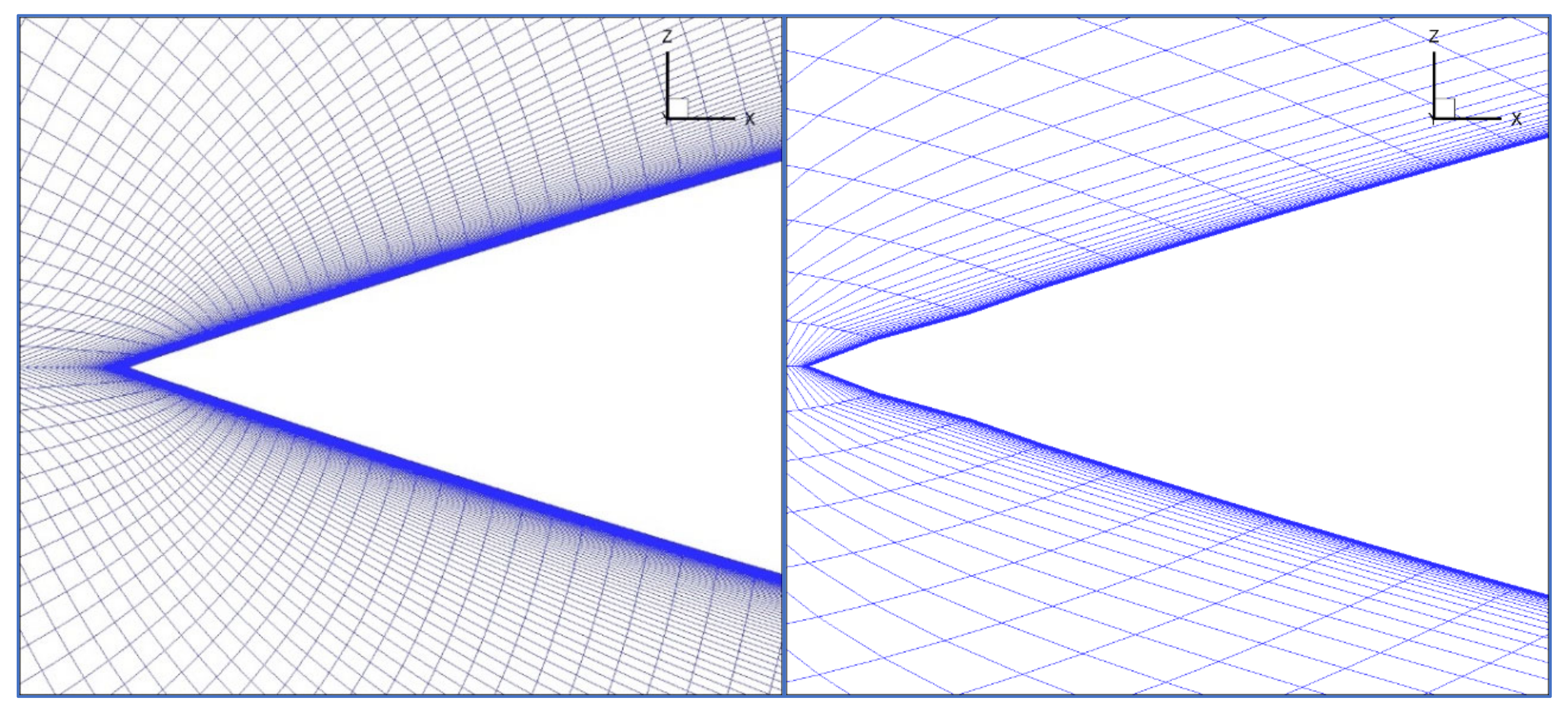
A two-dimensional structured grid was firstly generated. Then, a three-dimensional grid was generated by rotating this planar two-dimensional by steps of n degrees. The total number of cells in azimuth direction is $N=360/n$. This number N was chosen to be 240. The grid with 240 cells in azimuth direction was the grid utilized for the calculations. This grid has 450 cells in the longitudinal direction (x-axis direction) and 140 in normal direction. During the grid generation process, several tests regarding the distribution of the cells in longitudinal direction have been carried out. Special attention had to be paid to the grid resolution on the nose tip area. A detail of this is for two grids, shown in Figure 1 for the x-z plane. The grid on the left has a larger grid density at the tip. The next cell from the tip is at x/D ≈ 0.015 and the number of cells is large in a small region. The nose geometry is accurately resolved by this grid, but the mesh is coarser in the rear part of the body. The grid on the right has lower mesh density in the tip. The first cell from the tip is at x/D ≈ 0.045. The grid generation method, which uses splines interpolation for generating the geometry, has produced a small oscillation of surface curvature in the tip, which is not present in the theoretical model (3-caliber tangent ogive). Therefore, this second grid (coarse grid) resembles a smooth axisymmetric body with an axisymmetric irregularity at the tip. Grid S1 is represented by the right grid of Figure 1.

A detail of the structured grid (Grid S1) is shown in Figure 2. A stretching law is applied in normal direction. The height of the first cell to the surface was chosen as 10⁻⁵ m. With this value, the y⁺ was of order 1.

This structured grid is a fine mesh of approximately 15 million cells and 45 million faces. It has been used for some of the calculations whose solutions will be shown in this paper.

4.2. Unstructured Grid

The unstructured grid was generated with a very different methodology, using a method to generate a surface mesh of a part of the ogive-cylinder covered by an angle $(360/m)$ with m as an integer of any value. Values ranging from m = 3 to m = 8 have normally been used in the grid generation process. Additionally –in order to reduce the roughness at the nose tip- a mesh with m = 16 has also been generated. A maximum cell size is chosen, together with other parameters. This method implies that in the sections x/D very close to the tip, the grid is formed by a triangle if m = 3 and by an octagon if m = 8. When advancing in a longitudinal direction a cross section will be formed by polygons of many elements, which are closer to the ideal circular shape of the body. While every section was formed by 240 elements for the structured mesh, regardless of the radius of the circular section, for these unstructured meshes, the polygons are resolved by a different number of elements and their distribution is irregular. This results in non-axisymmetric meshes, with cross sections, which are different in number and distribution of the elements. To give insight of the implications of this type of meshing, a detail of the tip region for several unstructured grids is shown in Figure 3 for values of m = 3 and m = 8. The tip of the coarse mesh generated with m = 3 is very irregular. The tip of a grid generated with m = 8 is more regular, but not axisymmetric. Finally, the finer grid of the right looks more symmetric; however, a detailed examination shows differences at each azimuth angle. Therefore, neither of these grids are symmetric in the same fashion than the previously described structured grid.

For the majority of calculations, an unstructured grid named U1, generated by the methodology explained above, was chosen. The mesh size was of approximately 16 million cells. This grid was selected for comparison with the structured grid for several reasons: similar number of cells, computing time, level of roughness, etc. Regarding surface roughness, it is interesting to show the surface grid in sections close to the tip. The sections from x/D = 0.001 to x/D = 0.005 are formed by octagons with the elements distributed differently and also with different number of elements (see Figure 4 (left). There is a change from the section x/D = 0.005 to section x/D = 0.01, which is shown in Figure 4 (right)).

The section x/D = 0.01 is not an octagon, but a polygon with much more elements forming the surface mesh. The number of elements increases rapidly; the cross sections evolve more uniformly when advancing from x/D = 0.01 to x/D = 0.05.

The shape of the tip nose is very important for the final asymmetric flow pattern found at high angles of attack, and also for the roll angle dependence observed in the solutions. It may also be important for the determination of the angle of attack for onset of asymmetry.

An even finer mesh (U2) was also generated. The volume mesh has more than 38 million cells. This large mesh size was obtained due to a refinement of the surface grid in the ogive region and the use of m = 16 as the parameter for generating the surface mesh.

Similar cross sections at the tip nose region are shown in the following figures. The cross sections x/D = 0.001 to x/D = 0.005 are represented in Figure 5 (left) for this very fine mesh. The comparison with the same sections of the reference grid (see Figure 4 (left)) reveals that the approximation to an ideal circle is better, but it is also evident that the surface grid is irregular and not symmetric. The cross sections for x/D = 0.001 to x/D = 0.005 are represented in Figure 5 (right) for this very fine mesh. The comparison with the same sections of the reference grid (see Figure 4) is again revealing.

The tip nose of this finer mesh is smoother than that of the reference grid used for most of the calculations.

Hence, the two unstructured meshes differ in the level of roughness at the tip. Roughness and microscopic irregularities, particularly in the tip region, are sources of a convective instability and may induce an important effect of the roll angle in the normal and lateral forces on the missile, as it has been widely demonstrated in many experiments [2,5,7,8,10,21,22,23,24]. The tip surface roughness of the three generated meshes ranges from smooth (S1), low roughness (U2) to high roughness (U1), which allows for an investigation of the roughness effect on the flow field and the forces. It is worth noting that unsteady calculations with very small-time steps are required in order to achieve LES-like solutions with the SAS method, and, consequently, performing these simulations was a time consuming process, especially for Grid S2. Figure 6 provides a view of the surface mesh of Grid U1, and Figure 7 shows the mesh in two different cut planes, demonstrating that the grid is finest in the immediate vicinity of the body and that a cylindrical volume has been introduced around the body in order to better control mesh coarsening.

4.3. Numerical Roughness: Geometrical Similarity

Regarding the effects of irregularities, it is worth noting the work of Kumar et al. [8,21,22,23,24]. Experimental and numerical calculations have been done, adding perturbations of lower size than the boundary layer thickness in order to evaluate the effects of the roll angle on the forces. In reference [8], it is shown that the forces on a polished cone with roughness of the order of Ra~1 μm are different compared to the forces on a rough model of Ra > 6 μm. At high angles of attack, the polished cone shows a bi-stable pattern in the lateral or side force as a function of the roll angle. This is due to a global instability.

The rough cone shows a different sinusoidal form of the lateral force. At very high angles of attack, the force shows again the bi-stable pattern. At these angles the flow is basically unsteady and develops a ‘wave-like’ pattern; then, the effects of the imperfections are reduced. The cone tested in reference [8] has a diameter of D = 0.1 m. Then, the non-dimensional roughness is Ra/D = 1.5 × 10⁻⁵. The thickness of the local crossflow boundary layer close to the separation is of the order of 250–300 μm; i.e., δ/D ≈ 0.0025. For this test case, the Reynolds number based on the body diameter was Re_D = 0.3 × 10⁶, lower than the Reynolds number of our tests. Imperfections of the order of the crossflow boundary layer were introduced. The asymmetry increases significantly. In a numerical study [23], random imperfections of h/D = 0.004~2δ were introduced in the tip region and an increment of the lateral (side) forces was achieved.

These experimental and numerical studies show that imperfections of the geometry of boundary layer thickness size can produce significant increment of the flow asymmetry and then, large lateral (side) forces.

Before the calculations with the Grid U1 (see Table 1), an evaluation of the irregularities of this grid was carried out.

The differences between the locations of the surface mesh nodes and the ideal locations for a perfect circular shape at each cross section x/D was measured. These differences are shown in Figure 8 for two cross sections, x/D = 3.0 and 9.0. The blue lines are results on the port side and the red lines, the results on the starboard side.

These differences can reach values of h/D = 100 μm, i.e., h/D ≈ 10⁻⁴. This shows visually that the geometries of starboard and port side are noticeably different. In order to quantify these differences a ‘numerical roughness’ is defined in the following manner:

First of all, as the test model is a body of revolution, the average radius at each x/D section is defined as:

$$r_{avg}(x)=\frac{1}{N}{\displaystyle \sum _{i=1}^N{r}_i}(x).$$

Then, the ‘numerical roughness’ at each section is calculated by the following expression:

$$\overline{r_n(x)}=\frac{1}{N}{\displaystyle \sum _{i=1}^N}\left|r_i(x)-r_{avg}(x)\right|$$

(1)

This is an expression similar to that employed in [8]. The evaluations at different x/D sections of the reference unstructured grid show results of ‘numerical roughness’ between 40–60 × 10⁻⁶ m, i.e., r_n/D = 40–60 × 10⁻⁶ in the cylindrical part, while larger values were obtained for the ogive. It should be noted that Mahadevan [8] defined a rough model for values of Ra/D > 60 × 10⁻⁶. In addition, at reference flight conditions and an angle of attack of 45 degrees, the crossflow boundary layer thickness close to the separation point (at roll angles close to 90 or −90 degrees) was of the order of $\frac{\delta }{D}\approx 0.006-0.008$ at sections x/D = 3.0, 6.9 and 9.0. This value is larger than that measured in the experiment of reference [8], tested at a lower velocity and Reynolds number. We can conclude that the unstructured grid resembles a rough model.

5. Assessment of the Numerical Calculations

The calculations for the assessment process have been performed using the solver ANSYS Fluent^© [20] at the flow conditions defined in Section 2.

Abundant experimental information of the global forces, local forces and pressure coefficients ([14,15]), and also numerical information regarding the results obtained with several codes using different grids and turbulence models [15] exists, which was useful for comparisons.

The validation process consisted of several steps. First of all, calculations -both steady and unsteady- were carried out using standard turbulence models: the eddy-viscosity k-ω SST model and a ω-based RSM model. The next step was to employ the SAS method, performing simulations with both the k-ω SST-SAS and a ω-based RSM-SAS models. Most of the calculations were done for the structured grid (Grid S1). Transient calculations were carried out, using small-time steps of Δt = 5 × 10⁻⁴ s. Results were recorded for a period of T = 4 s.

We concluded that only the RSM-SAS model was adequate to capture the main flow features: the existence of two differentiated flow regions, i.e., a steady flow region in the fore body (region 3 defined by Ramberg and Degani et al., references [11,12,13]); and an unsteady flow region at the rear (region 2). A region 1 similar to the von Karman vortex street was not present due to the low fineness ratio (L/D < 16). Other numerical studies carried out by the authors for a configuration with larger fineness ratio have confirmed the existence of this region 1, where the averaged local side force is close to zero. Due to the fineness ratio, the local side force is damped in the rear part of the body. Only the method which uses the RSM-SAS turbulence model was capable to capture this damping. In general, the results were good and showed better accuracy than the numerical solutions shown in reference [15].

The fluctuating nature of the flow, as well the two distinct regions, are shown in Figure 9 and Figure 10.

The time history of the global force coefficients is plotted in Figure 9. While the normal force coefficient (blue line) experiences small fluctuations, the fluctuations of the side force (red line) are important, ranging from the smaller values of 2 to values close to 4, with an averaged value of 2.99 within this period (T = 4 s). The fluctuations of the normal force are one order of magnitude lower. A Power Spectral Density (PSD) analysis of the forces shows energy content for frequencies below 20 Hz, with 7.3 Hz being the dominant frequency for the side force coefficient, indicating a Strouhal number of 0.150. In reference [15], it is mentioned that the experimental Strouhal number for this test case was 0.160.

Several solutions for the local side and normal force coefficients, at different times within a transient period of T = 0.1 s, are shown in Figure 10. The dot black circles denote experimental data. There is a steady flow region in the nose region, extending from the tip up to x/D ≈ 7.0. In addition, a rear unsteady flow region exists where the forces oscillate. This flow pattern coincides with the observations of Ramberg in many experiments [11]. According to Bridges (see reference [9]) and Degani et al., (references [12,13]), for bodies of fineness ratio below L/D = 16 there are only two flow regions: one steady flow region (region 3); and another unsteady flow region where periodic shedding of vortices inclined obliquely to the longitudinal axis is observed (region 2) and where the local side force decays, but have a non-zero mean value. For bodies with a fineness ratio larger than 20, there may exist a third unsteady flow region (denoted region 1) where a von Karman vortex street type flow occurs and where the average local side force is zero.

The solutions obtained with the standard turbulence models (k-ω SST and RSM) did not capture the two different flow regions, and therefore an unsteady local side force with a damped amplitude was not observed in region 2 (at the rear body). The numerical solution described a steady flow: in fact, the RSM model captured a small fluctuation of the flow at the rear but with a frequency of one order of magnitude lower than that obtained with RSM-SAS. Surprisingly, the solution obtained with k-ω SST-SAS was very different to that of RSM-SAS model; it was qualitatively similar to that of the standard RSM model. The solution was steady and the local force coefficients did not show damping at the rear. This was an unexpected result, since the solutions obtained by this model for a cylinder in crossflow are very accurate when compared to the experimental data, and are also very different to those of the standard k-ω SST model [17].

The key argument for an explanation about this feature is given by the authors of the method –Menter amd Egorov- who say that SAS relies on an instability of the flow to generate resolved turbulence. In cases where such an instability is not present, the model will remain in RANS mode [18]. Another possibility is that the grid is coarse and the time steps are large (leading to CFL >> 1). In this case, SAS will run in RANS mode [16].

However, for the RSM-SAS solutions an unsteady flow region at the rear has been captured, showing the damping of the local forces (see). The grid and time steps used are the same as those used for the k-ω SST-SAS model. Therefore, there is some numerical mechanism using this non isotropic model, which produces sufficient instability in the flow to activate the Scale Resolving Mode, which is capable to compute turbulence scales up to the grid size limit. Then, LES-like solutions are possible in the unstable region, i.e., the region at the rear part of the body. In addition, in the steady flow region (nose region) the side and normal forces fit better to the corresponding experimental values, indicating that the vortices were captured more accurately, which contributes to an increased accuracy of the normal and side forces.

It is very illustrative to check Figure 11, where the iso-surfaces of the Q function are plotted for the two different SAS models used. Q function is the second invariant of the velocity gradient tensor and can be defined as: $Q=0.5\times \left({\omega }^2-S^2\right)$ where ω is the norm of the vorticity tensor, an S is the norm of the strain rate tensor [25].

The iso-surfaces are colored by turbulent viscosity ratio. They help to determine coherent vortex structures. Positive Q-function values indicate areas where the rotation overcomes the strain, making it possible to identify these surfaces as vortex envelopes [25]. It is very important to notice that the turbulent viscosity ratio in the vortex structures is one order of magnitude lower when using the RSM-SAS model, when compared to the solutions obtained with the k-ω SST-SAS model. This is a clear indication that with the latter model, RANS-like solutions are obtained, since a reduction of turbulent viscosity cannot be observed. URANS methods are overly dissipative, since all turbulent scales are modeled and only frequencies far lower than those of turbulent fluctuations are resolved [18]. This is the reason for them being less accurate in computations of unstable or transient flows. The fact that the reduced turbulent viscosity results are obtained with the RSM-SAS model indicates that large turbulent scales are resolved and LES-like solutions are obtained.

Therefore, the use of an advanced turbulence model, as RSM-SAS combined with a grid fine enough and small-time steps have permitted to capture the main features of the flow for this type of configuration at a high angle of attack. The time step is very important in order to achieve CFL values close to 1. Otherwise, this would lead to a steady RANS solution.

Thus, the concern regarding the k-ω SST-SAS model is to check if the model would run in Scale Resolving Mode at a higher angle of attack, as the results given in [18,19] for a cylinder in crossflow showed good results for this model. There may exist a critical angle of attack larger than 45 degrees for which the flow is sufficiently unstable to activate LES-like mode. Menter et al., mentioned that one possibility for CFD calculations in such cases (below the critical angle) is to generate synthetic turbulence [18].

Concluding, the RSM-SAS model seems to be a high-level turbulence model capable of capturing two separated flow regions, one steady flow region at the nose, and another unsteady flow region at the rear, which is in agreement with the findings of several authors, which studied the experimental data of axisymmetric bodies of moderate to high fineness ratio [9,11].

6. Effect of Angle of Attack: Influence of Roughness

The results obtained at the test conditions with the two grids (Grids S1 and U1) indicate that the roll angle has an important effect on the forces if the unstructured grid is used. There is experimental evidence of the influence of the roll angle on the forces for this ogive-cylinder configuration at other conditions of Mach number Ma = 0.5 and Re_D = 0.3 × 10⁶ [2]. The influence of the roll angle clearly stems from a non-axisymmetric structure of the mesh and to the surface roughness. An average roll angle side force coefficient can be calculated as:

$$\left|C_{Yavg}\right|=\frac{1}{N}{\displaystyle \sum _{i=1}^N\left|C_{Yi}\right|}$$

The different values of $\left|C_{Yi}\right|$ are obtained by calculating the side force in N different directions. The resulting value for Grid U1 and N = 8 is $\left|C_{Yavg}\right|=2.472$. When the structured (and symmetric) Grid S1 is used, no roll angle effect is observed. Two possible mirror solutions of different sign and equal magnitude exist for each roll angle. Which of the two possible mirror solutions is obtained depends on initial conditions or some numerical perturbations in the initial stage.

There is another effect of the roughness: the angle of attack for onset of asymmetry is lower for the rough model than for the smooth model. This angle was about 25 degrees for the smooth model and 15 degrees for the rough model at the reference flight conditions, according to references [2,14]. At other Reynolds numbers, also at laminar flow conditions, this angle for onset of asymmetry is always larger for the smooth model, indicating the strong effect of the convective instability due to surface roughness or other body imperfections. Relevant information for this study is shown in reference [14]. The curves of normal and side forces are different for the smooth and rough models tested at the same facility and flow conditions. This shows clearly the effect of roughness –at a fixed roll angle in this case- on the forces at the different incidences. The angles for the onset of asymmetry are different for each model. Then, to numerically quantify this effect the angle of attack was varied from 10 degrees to 45 degrees. The solution for the structured Grid S1 -in terms of global force coefficients- is given in

Table 2. Side and normal force coefficients versus angle of attack: Ma = 0.2, Re = 2 × 10⁶. Grid S1.

α (deg.)	CY	CN
10	−0.0006 ± 0.13	0.57 ± 0.027
20	−0.0005 ± 0.17	1.71 ± 0.019
30	0.13 ± 0.14	3.33 ± 0.065
32.5	−0.039 ± 0.24	3.83 ± 0.150
33.5	0.038 ± 0.24	4.06 ± 0.165
34.0	0.136 ± 0.31	4.36 ± 0.122
34.5	−2.92 ± 0.43	5.66 ± 0.190
35.0	2.79 ± 0.23	5.69 ± 0.076
40.0	2.81 ± 0.29	6.85 ± 0.090
45.0	2.99 ± 0.27	7.77 ± 0.100

, and the solution for the unstructured Grid S1 at the roll angle of Φ = 0 deg. is shown in

Table 3. Side and normal force coefficients versus angle of attack: Ma = 0.2, Re = 2 × 10⁶. Grid U1.

α (deg.)	CY	CN
20	−0.07 ± 0.09	1.73 ± 0.010
25	−1.80 ± 0.05	2.69 ± 0.014
30.0	−1.96 ± 0.06	3.89 ± 0.050
35.0	1.32 ± 0.28	5.90 ± 0.090
40.0	2.19 ± 0.42	7.31 ± 0.120
45.0	3.22 ± 0.35	7.80 ± 0.120

. As observed in Table 2 the side force stays at small values up to an angle of attack of 34 degrees. At 34.5 degrees there is a sudden jump to larger values and beyond that the side force remains in the same range even for the angles of 40 and 45 degrees, showing a ‘plateau region’ which is also seen in the experimental data. The data of Table 3 indicate asymmetric flow at 25 degrees.

The numerical data of the structure Grid S1 were compared to the experimental data of the smooth model [14]. The plots for the side force coefficient versus the angle of attack are given in Figure 12 (left side) while the results for the normal force coefficient are plotted in the right side of Figure 12. It is important to remark that for comparison with the experimental data, the negative numerical solutions –one of the two specular solutions- for the side force coefficient were used.

Champigny [2] gives a value of angle of attack for onset of asymmetry of 15–20 degrees for the smooth model, however the experimental data in Figure 12 indicate the existence of a slight flow instability at 20–30 degrees, with the side force oscillating between negative and positive values (the two possible solutions for a bi-stable pattern). At approximately 35 degrees, an abrupt change can be observed, followed by a steep slope of the curve between 35 and 40 degrees. At 50 degrees, a change from the negative solution to the positive solution can be noted, likely due to the test conditions. As mentioned before, there are two mirror solutions, one of negative sign and the other of positive sign. Beyond this angle, there is a damping of the side force. The flow is basically ‘wake-like’ and unsteady with a small region in the nose of steady asymmetric flow.

Regarding the numerical simulations, an abrupt change from a quasi-symmetric steady flow solution at 34 degrees to an asymmetric unsteady flow solution at 35 degrees is clearly observed.

This change from symmetric to asymmetric flow is also evident in the normal force coefficient curve of Figure 12 due to a noticeable increase of the curves slope between 34 and 35 degrees, which is the angle of attack for the onset of asymmetry identified before. The values of the side force at 35, 40 and 45 degrees are similar, following the experimental trend which anticipates a variation in the local side force pattern, changing from 3 to 4 maxima of the sinusoidal curve. This also becomes evident in the observed decrease of the slope of normal force curve at these angles. The semi apex angle for this ogive is δ_n = 18.94 deg., thus the empirical angle of attack for onset of asymmetry is α_onset = 37.88 deg. This is close to the value obtained numerically, and in the experiments (see Figure 12).

Regarding the solutions obtained with the unstructured Grid U1, the numerical values of the side force coefficient and the normal force coefficient are compared in Figure 13 left and right, respectively, with the corresponding experimental data of the rough model [14]. Again, the negative numerical side force solutions were used for comparison with the experimental data. The experimental data clearly show an onset of asymmetry for an angle of attack below 20 degrees. At an angle of attack of 20 degrees the side force is significant. According to Champigny [2], the value for the angle of attack of onset for asymmetry may lie between 12 and 15 degrees. According to this numerical simulation, this onset occurs between 20 and 25 degrees. The increase of the normal force slope at an angle of attack for onset is not as large as that of the experimental smooth body or that of the structured grid solution. However, the angle of attack of onset for asymmetry is smaller than that of the smooth body, indicating that the surface and flow irregularities trigger the appearance of asymmetric flow disturbances. It is worth noting that the experimental side force (absolute value) is larger at 20 degrees than at 25 degrees. After this, the side force increases its absolute value, until reaching a maximum at 50 degrees. The reason of this behavior lies in the variation of the local side force coefficients along the longitudinal coordinate.

In reference [2], the curves of the experimental local side force coefficients of the rough model are plotted for the angles of attack 20 to 60 degrees. At 20 degrees, the local side force has a wavy form with two peaks before reaching the end of the body. At 30 degrees there are three maximum values. This results in a local minimum of the overall side force at 20 degrees due to the change from one maximum to two maxima, due to alternating positive and negative local contributions to the overall side force. At 40 degrees a fourth peak appears. The base condition breaks down resulting in a fifth peak at 45 degrees. The unsteady wavy flow region advances from the rear to the nose as the angle of attack increases. At 45 degrees, this unsteady region covers the rear part of the body. The experimental data at 50 degrees indicate a similar form of the curve than at 45 degrees but as the unsteady region advances, the local side force is damped and the overall side force reaches a maximum. After 50 degrees, the value of the global side force is reduced when compared to the maximum values at 45–50 degrees. At 55 degrees, the local side force has 6 peaks and the unsteady region is dominant, except for the nose region. A strong reduction of normal force appears between 50 and 65 degrees. At these conditions, there must be an alternating von Karman vortex street in the rear part, with an average side force zero. The remaining side force results only from the nose contribution. The strong impact of roughness also becomes evident by investigating the solutions obtained with the finer unstructured grid (Grid U2). As it was shown above (chapter 4), this grid was much finer in the ogive region, leading to an important increment of the surface mesh there and a volume mesh more than double size than the reference unstructured Grid U1 (see Table 1).

The solution for the finer unstructured grid at a roll angle of Φ = 0 deg. is shown in

Table 4. Side and normal force coefficients versus angle of attack: Ma = 0.2, Re = 2 × 10⁶. Grid U2.

α (deg.)	CY	CN
20.0	0.09 ± 0.0072	1.74 ± 0.0084
25.0	−0.06 ± 0.0597	2.49 ± 0.0111
30.0	−1.39 ± 0.1976	3.80 ± 0.0681
35.0	−1.37 ± 0.2490	5.60 ± 0.0773
40.0	−2.24 ± 0.4718	7.42 ± 0.1304
45.0	−2.01 ± 0.4768	8.32 ± 0.1368

.

Regarding the unstructured grid solutions, the numerically obtained values of the side force coefficient and normal force coefficient are compared in Figure 14 left and right, respectively, and are shown together with the corresponding experimental data of the rough model [14]. Again, the negative numerical side force solutions were used for comparison with the experimental data. The red squares are the solutions for the Grid U1, while the green squares represent the solutions given in Table 4. According to this numerical simulation, the angle of attack for the onset of asymmetry occurs between 20 and 25 degrees for Grid U1; but for the Grid U2, this angle lies between 25 and 30 degrees. In both cases, these angles are smaller than that of the structured grid (Grid S1), which resembles a polished model with very low roughness. As the Grid U2 has a lower numerical roughness in the ogive region, these results indicate a delay in the angle of onset of asymmetry, approaching to the one obtained with the structured Grid S1 (~35 degrees). The shape of the side force curve seems to follow the trend of the experimental curve and of the other numerical curve with one exception. A larger side force coefficient (in magnitude) would be expected at 45 degrees if the curves were to reproduce the trend of the experimental data with a delay.

In order to investigate the load distribution, 10 local side and normal force coefficients calculated at an interval of T = 0.5 s (the last part of the transient period) have been plotted in Figure 15 together with the averaged values (blue lines) and experimental data (black dots). The local curves indicate that in the region x/D < 6–7 the flow is steady, although some oscillations in the normal force coefficient appear. This is the region 3 defined by Ramberg (see [11]). The rear part of the body develops an unsteady asymmetric flow, where the local side force is damped when advancing towards the back. It is worth noting that we have used a period of T = 0.5 s for taking the average, while for the averaged force coefficients of the curves shown in the period was T = 0.1 s. The PSD analysis within the transient period of T = 2 s indicated a dominant frequency below 10 Hz. A comparison of the averaged curves of the Grid U1 and of the Grid U2 with the experimental data is given in the Figure 16.

Before comparing the curves, it is worth noting that the study of the forces at different roll angles for the Grid U1 gave values for the side force coefficient that range from a minimum of 1.94 (at Φ = 45 deg.) to a maximum of 3.22 (at Φ = 0 deg.) in terms of absolute values. A similar roll angle-dependent investigation for Grid U2 has not been performed, but at the roll angle of Φ = 0 degrees the global side force coefficient is 2.01 (absolute value, see Table 4). This value is within the envelope of solutions obtained for the Grid U1 for the different roll angles. It is evident that roughness produces a large variation of the side force, ranging from 1.94 to 3.22, i.e., a difference of more than 50%. Liaño [26] pointed out that: “since the integrals are the balance of positive and negative zones of the oscillating curves, small cumulative differences of the sectional forces yield important deviations of the overall side force.”

It is evident that both longitudinal side force distributions follow the same pattern; a sinusoidal curve with 5 peaks denoting the alternating vortex shedding structure. However, the flow in the tip is different and that produces a delay in the asymmetric flow for the finer mesh (Grid U2). This affects the global force coefficient greatly. It is also remarkable that larger normal forces just in the cylindrical part coefficient close to the ogive is solely responsible for the larger normal force coefficient obtained for Grid U2. This has a clear influence on the normal force coefficient. As shown in reference [26] the detached zone contributes mainly to the normal force coefficient, while the attached zone contributes mainly to the side force coefficient. Then, a structure with stronger vortices must have been developed in this part, induced by the higher level of roughness.

In conclusion, all the calculations performed indicate a large effect of roughness in the pressure field and therefore both in local and global force coefficients, when the flow is at high angles of attack conditions.

Every study for a design of a slender body of revolution configuration for low-speed conditions must take into account the level of roughness, as well other important geometrical features such as bluntness. The different forces obtained will form a design envelope, useful for control dimensioning.

7. Conclusions

The flow past an axisymmetric body at a high angle of attack and low velocity is a challenging problem for numerical simulations. This type of flow develops characteristics of an unsteady asymmetric flow. A dependence of the forces on the roll angle has been observed in several experiments, provided the body has geometrical irregularities. Only the calculations with Reynolds stress turbulence models and the Scale-Adaptive Simulation method (RSM-SAS) captured the main features of the flow, contrary to other eddy-viscosity turbulence models or standard Reynolds stress turbulence models. These models are too diffusive and were not capable to detect the unsteady nature of the flow at the rear body and to capture small turbulent scales, unlike the RSM-SAS model. The use of LES methods for these high Reynolds flows is very time consuming. The RSM-SAS turbulence model has been demonstrated to be capable to obtain LES-like solutions, a very important feature in order to carry out studies of missile type configurations at high angles of attack.

The use of fine meshes, and performing transient calculations with small-time steps, was necessary and imperative. The comparison of the results obtained with a structured axisymmetric grid and an unstructured grid -which shows geometrical irregularities in the tip nose together with other microscopic irregularities- has been shown to be fundamental in order to check the influence of the geometrical irregularities for the existence of a convective instability, which is added to a global instability at high angles of attack.

A relevant conclusion is that, by using a structured grid, it is possible to reproduce solutions close to the experimental values and which reproduce the experimental observations for a polished model. As expected from symmetry considerations, the roll angle of the missile with respect to the free stream direction has no relevant effects on the results and there is an angle of attack for onset of asymmetry. A global instability leads to a bi-stable pattern of two equivalent specular asymmetric flow solutions, one mirror of each other. The flow field on the rear part of the body is unsteady, with the amplitude of the oscillations increasing with the angle of attack. In the fore body the nose effects are dominant and there is a steady asymmetric flow. Flow instabilities lead to an asymmetric flow pattern from the tip on.

Since the surface mesh of the unstructured grid has some irregularities resembling the roughness of an irregular body, a convective (or spatial) instability could be reproduced, and its effect is to reduce the angle of attack for onset of asymmetry. This effect is added to the global instability.

The comparison of the local and global forces obtained with the structured and unstructured grids, with experimental data corresponding to polished and rough models, respectively, is qualitatively good. The numerically obtained angles of attack for the onset of asymmetry are different than the experimental values, but the qualitative trends of the normal and side force curves are captured with fair agreement.

A CFD study seeking grid independent solutions is only expedient for structured grids, which are intrinsically symmetric and have a very low level of roughness.

Regarding the missile design process, for which the dimensioning of the control fins is required, a study with several grids, either structured symmetric or unstructured asymmetric, is more appropriate. It is likely that different loads should be predicted at the same flow conditions. An envelope of solutions could be obtained. The size of control devices should be calculated using the extreme values of the envelope of loads.