Receding Horizon Trajectory Generation of Stratospheric Airship in Low-Altitude Return Phase

Abstract

The contribution of this paper is the proposal of a new receding horizon trajectory generation method for stratospheric airships’ return phase. Since the energy consumption, wind field and path constraints are restrictions during the return phase of airships at low altitude, it is crucial to develop novel trajectory optimization methods to ensure that the airship returns to the landing site. In this article, optimization objects and conditions of the return trajectory were constructed, considering the energy consumption and wind field. Then, a modified interior point method (MIP) was used to transform the inequality constraint, which is a simple and adaptable method used to improve the solving efficiency on the basis of a modified multiple shooting method (MMS). In addition, an adaptive gradient descent regulator was improved to reduce the influence on the optimization result due to different selections of the initial search point, and the convergence was made faster and more stable. Finally, considering the performance and path constraints of the airship, the effectiveness of the scheme was verified by numerical experiments under wind effects and a comparison of different methods.

1. Introduction

Stratospheric airships can extend the duration of the flight time (over a month) at near-space altitude (18–22 km) based on buoyancy and propulsion systems. Based on the advantages of a long endurance, large carrying capacity and wide work coverage, airships as a stratospheric real-time monitor or space transmission platform have attracted wide attention [1,2,3,4,5,6], having important applications in the fields of earth observation, emergency rescue and civil communication, etc. [7,8,9,10,11].

Stratospheric airships rely on the lift generated by lighter-than-air gases such as helium to maintain being stationary in the air, and altitude changes can be realized through ballonet valves opening and closing. The near-space region is approximately a quasi-zero wind area, having a small wind force. However the wind is very strong at low altitude. Thus, the applicable propulsion system is required to be different in the two regions. Based on this, the wind field, prescribed flight range, low-altitude propulsion system and forbidden region become constraints for the process of airships landing. A main challenge in the airship landing process is the planning and optimization of the airship’s descent trajectory.

The airship descent process is mainly divided into two steps: early-stage descent and low-altitude return, respectively, shown in Figure 1. The first step is to release the lighter-than-air gas in ballonets, reducing the buoyancy of the airship, and to drop rapidly through the troposphere. The second step is to abandon the ballast, decreasing the descent speed of the airship at an altitude of 3 km. Then, the low-altitude propulsion system is activated to bypass the forbidden region and reach the landing site within the designated flight range. In this process, the goal of trajectory optimization is the low-altitude propulsion system energy consumption and flight time, and the limiting factors are path constraints and the wind field. However, very little research has been conducted in this area so far [12,13,14,15].

Zhang and Li [16] studied an energy optimization problem based on the position potential method to improve the duration time of airships, and conducted a case study to validate this strategy. A three-dimensional optimal trajectory design was addressed for a stratospheric airship platform, considering a real jet stream and flight constraints [17]. However, path constraints such as forbidden zones were not addressed. Zhu and Li [18] aimed to improve the solar energy system of a near-space airship by optimizing the airship yaw angle. The recovery trajectory optimization of the stratospheric airship was discussed to find the economical recovery flight trajectory to the station-keeping site [19]. Lanteigne and Blouin [20] transformed the optimal trajectory problem into an optimal control problem and solved it using a pseudo-spectral method, providing a reference for the numerical optimization of trajectory. Although these methods [21,22,23,24,25] can also obtain airships flight trajectories, there seem to be some limitations.

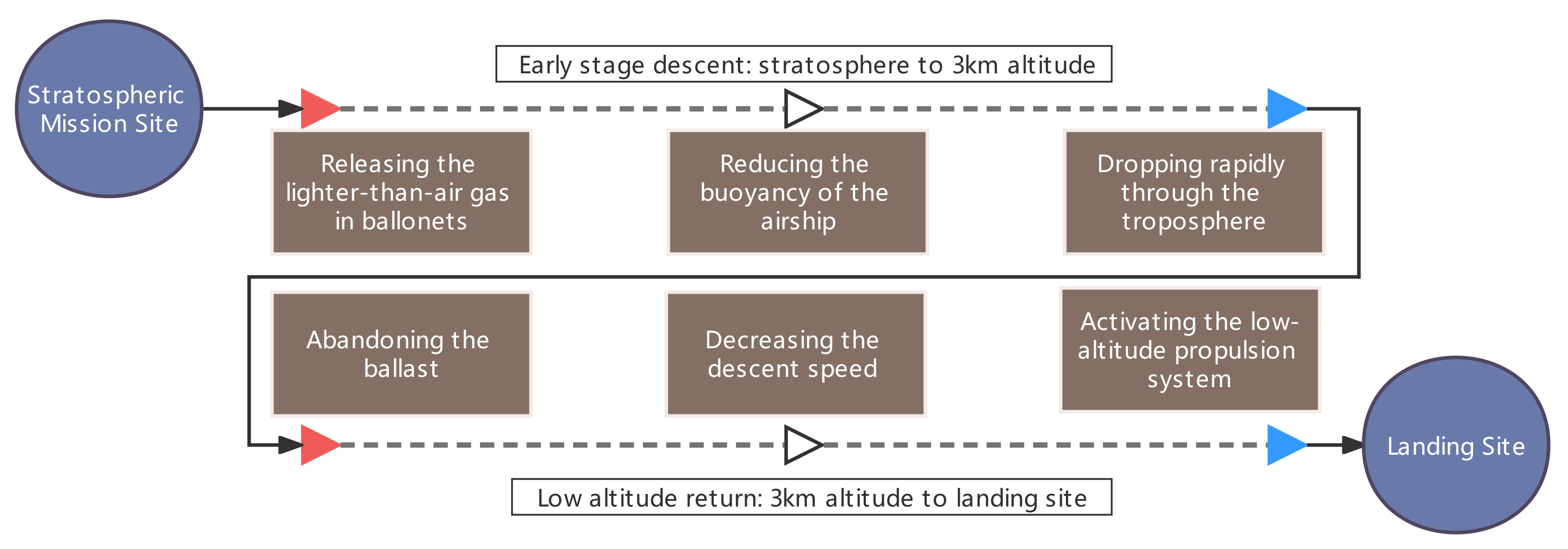
• As described above, the influence of the wind field is mainly considered in the stratosphere, and trajectory generation in the low-altitude region is not covered.
• In previous studies, the limiting factor is mainly considered as the wind field, while the path constraint is not mentioned.
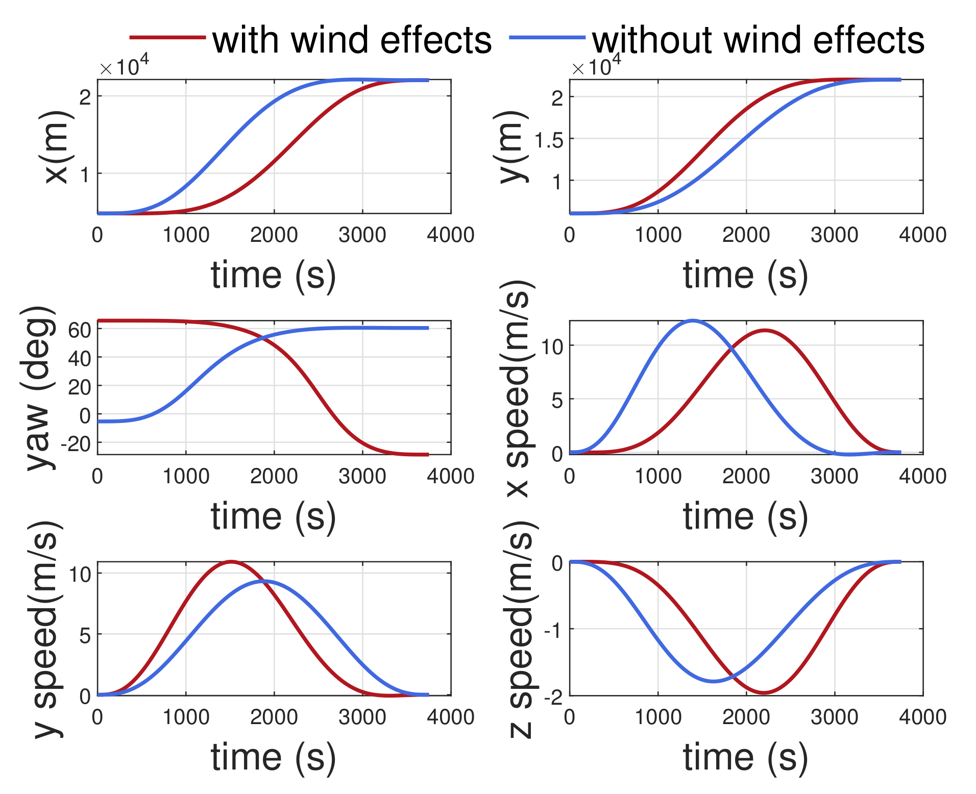
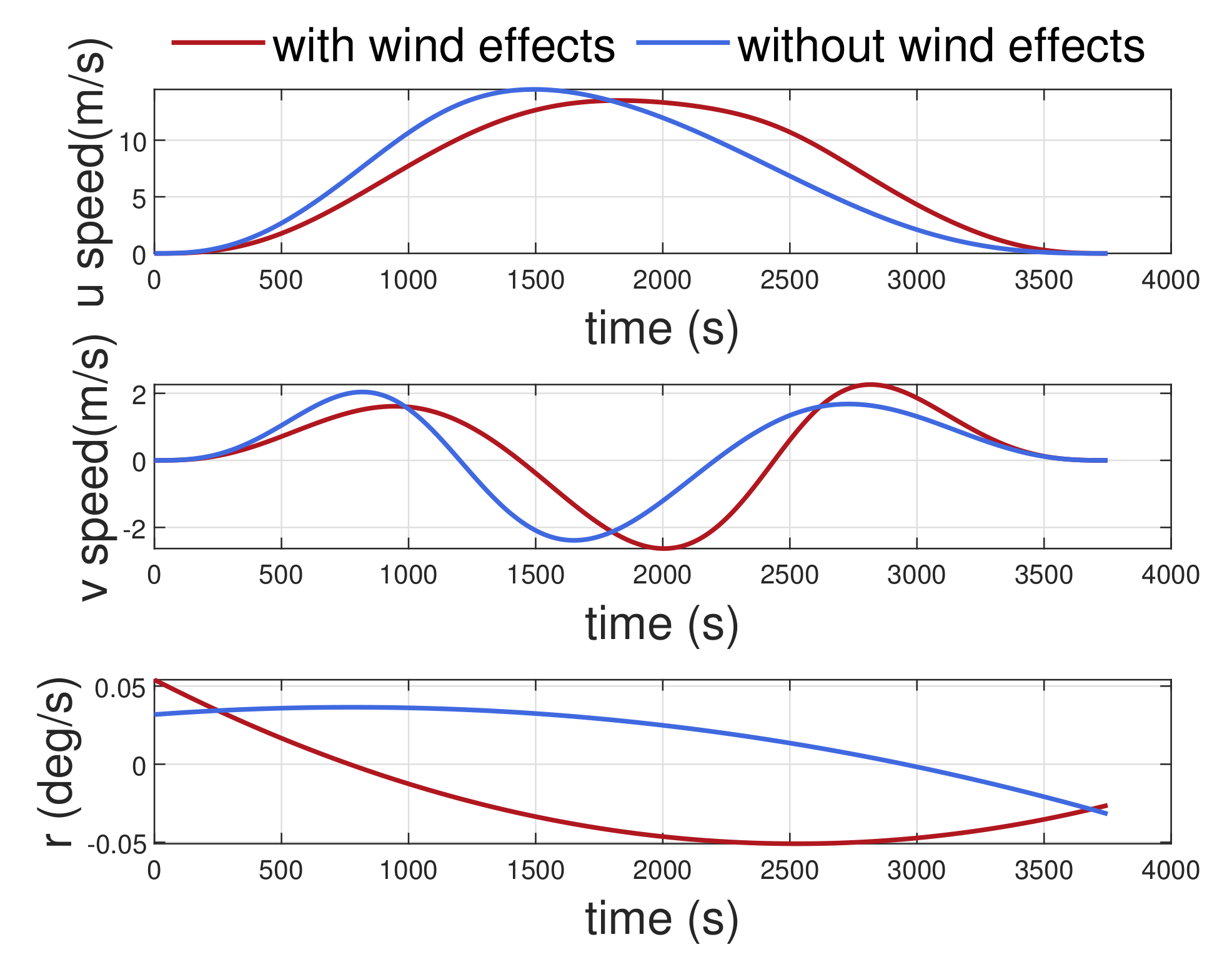
• The airship is an aircraft with large inertia, and its state cannot be changed rapidly. The trajectory generated by many studies is not smooth; for example, the speed and attitude change rapidly in a short time, which will challenge the propeller and structure of the airship.

This paper takes the low-altitude return phase as the research background, expresses the limiting factors, and proposes a modified simple-structure and efficient numerical optimization method. The main contribution of this paper can be summarized as follows.

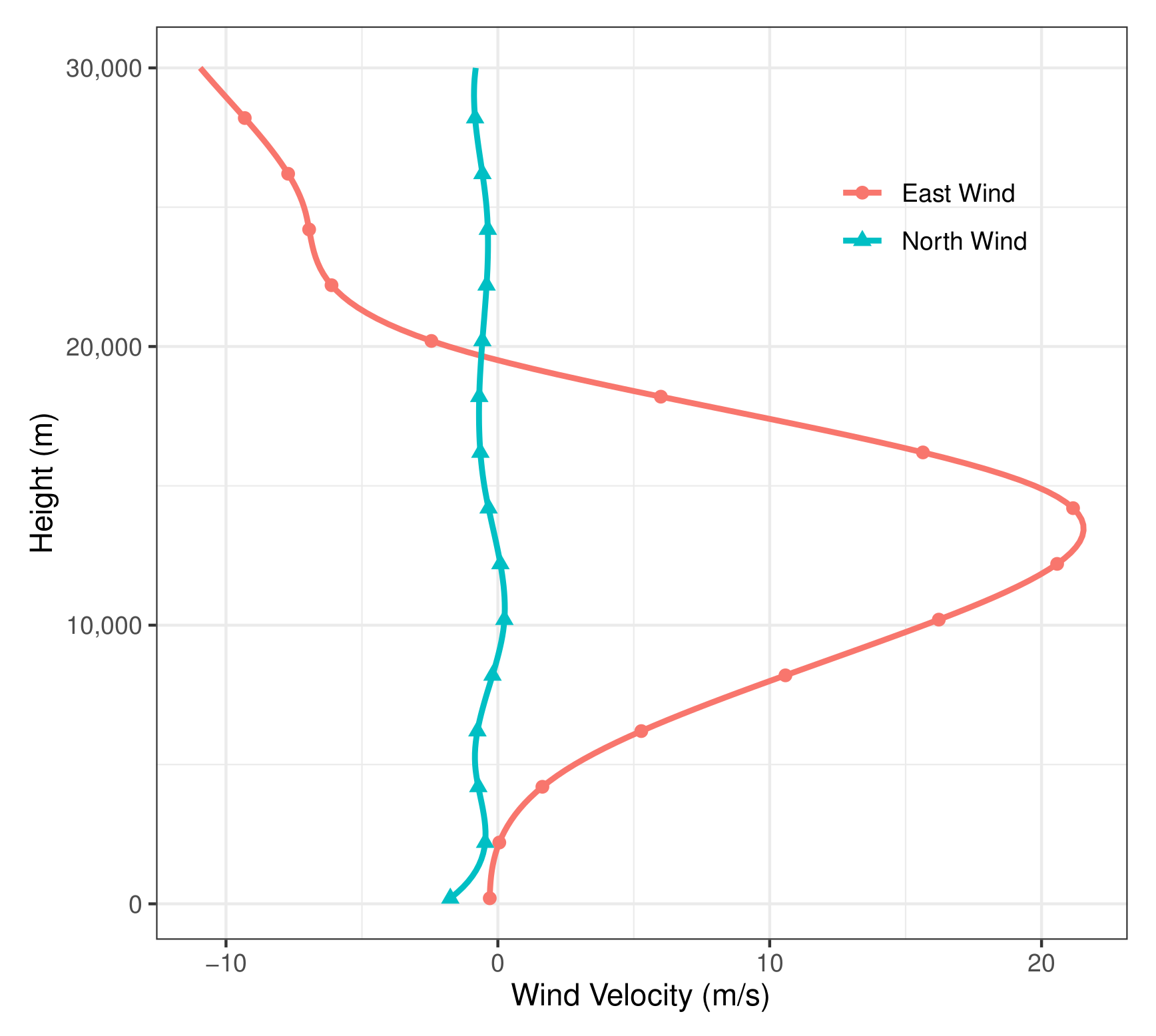
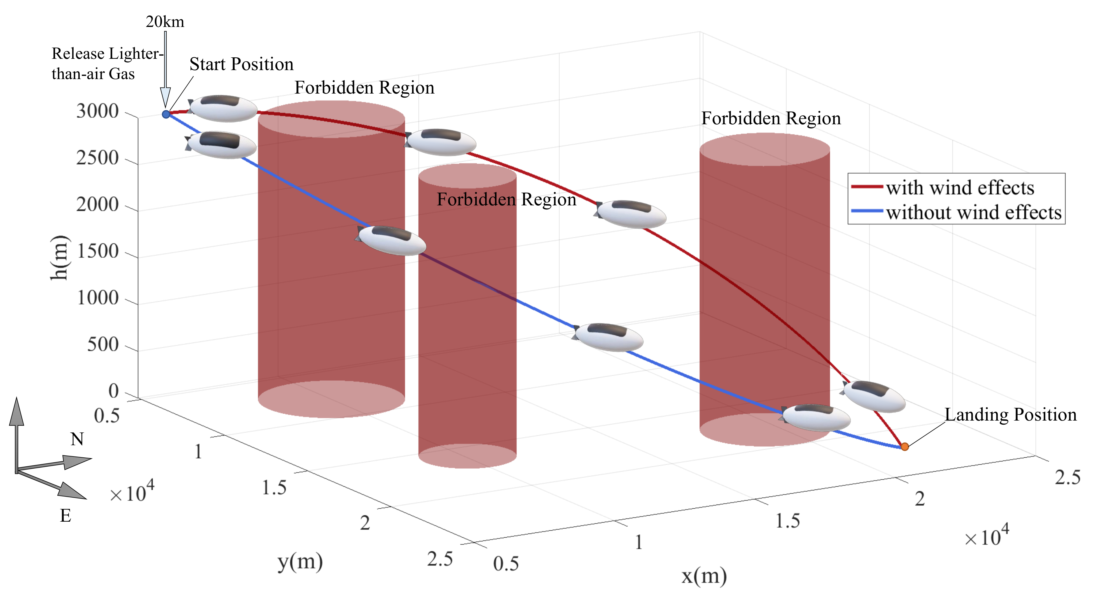
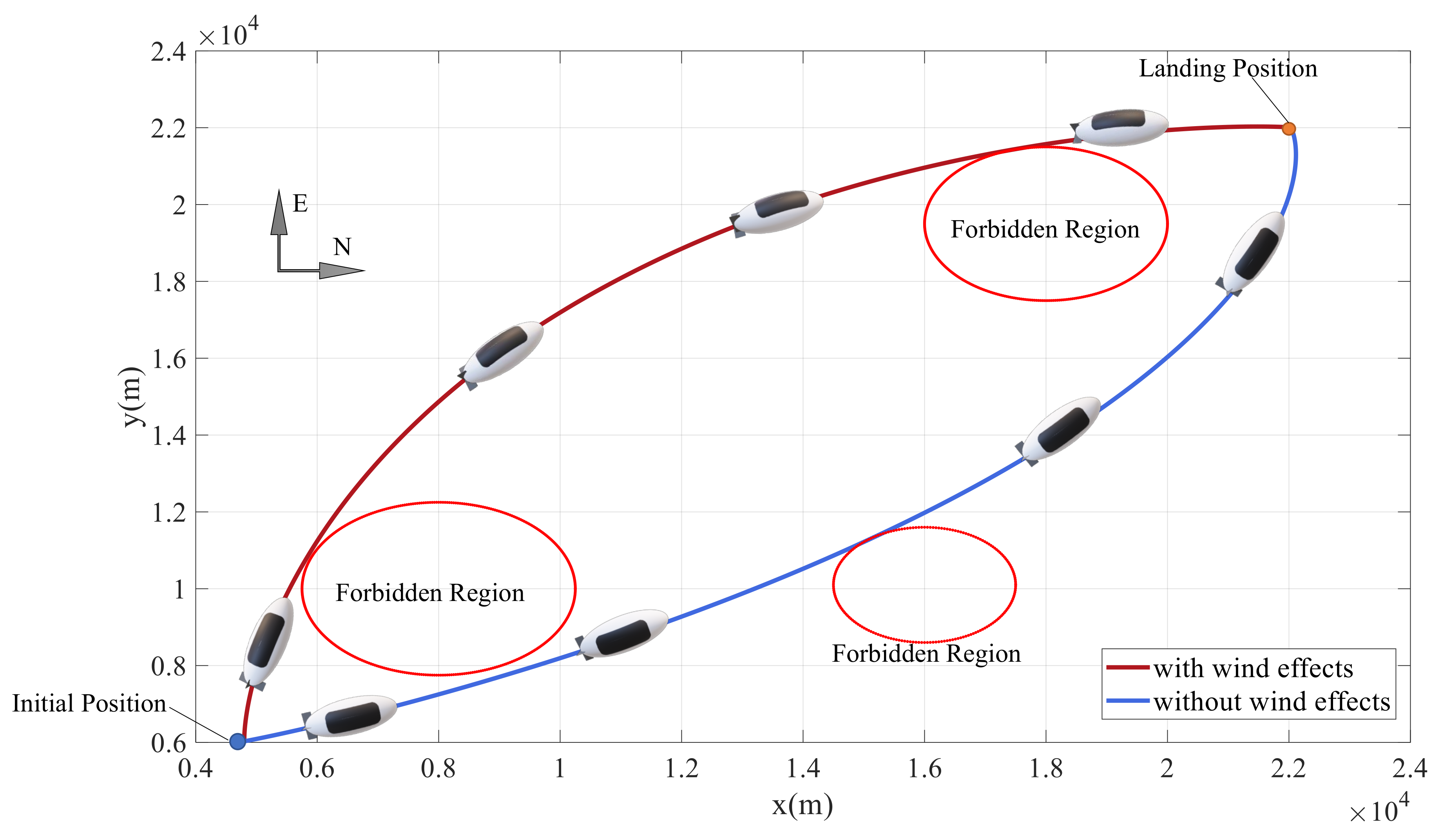
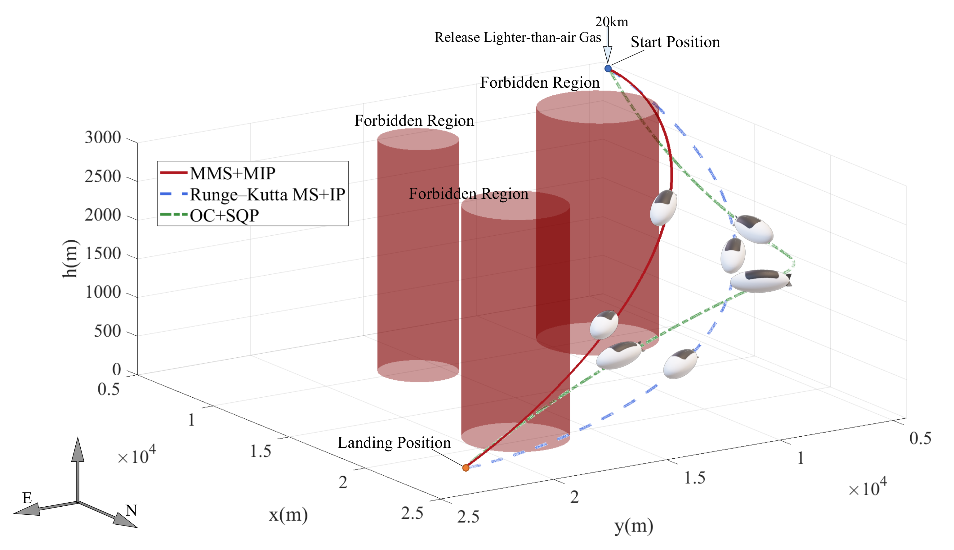
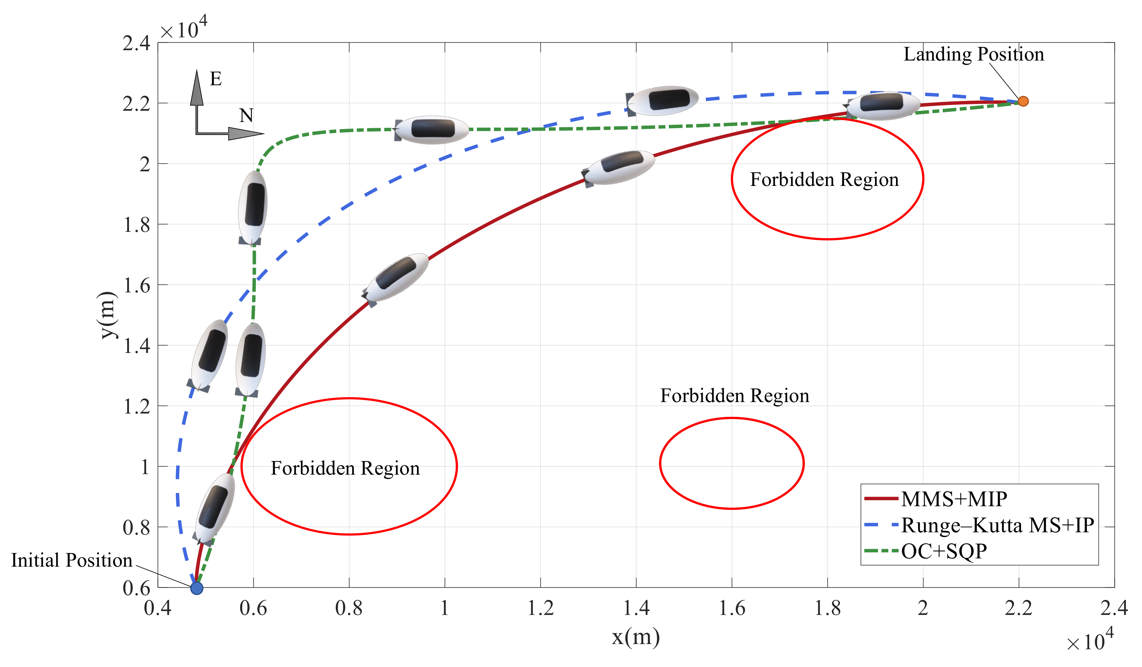
• The vertical wind shear model and constant wind model at different altitudes were established according to the wind field data results. The landing site, wind field, forbidden region and flight range were transformed into a terminal constraint, penalty function and path constraint, respectively.
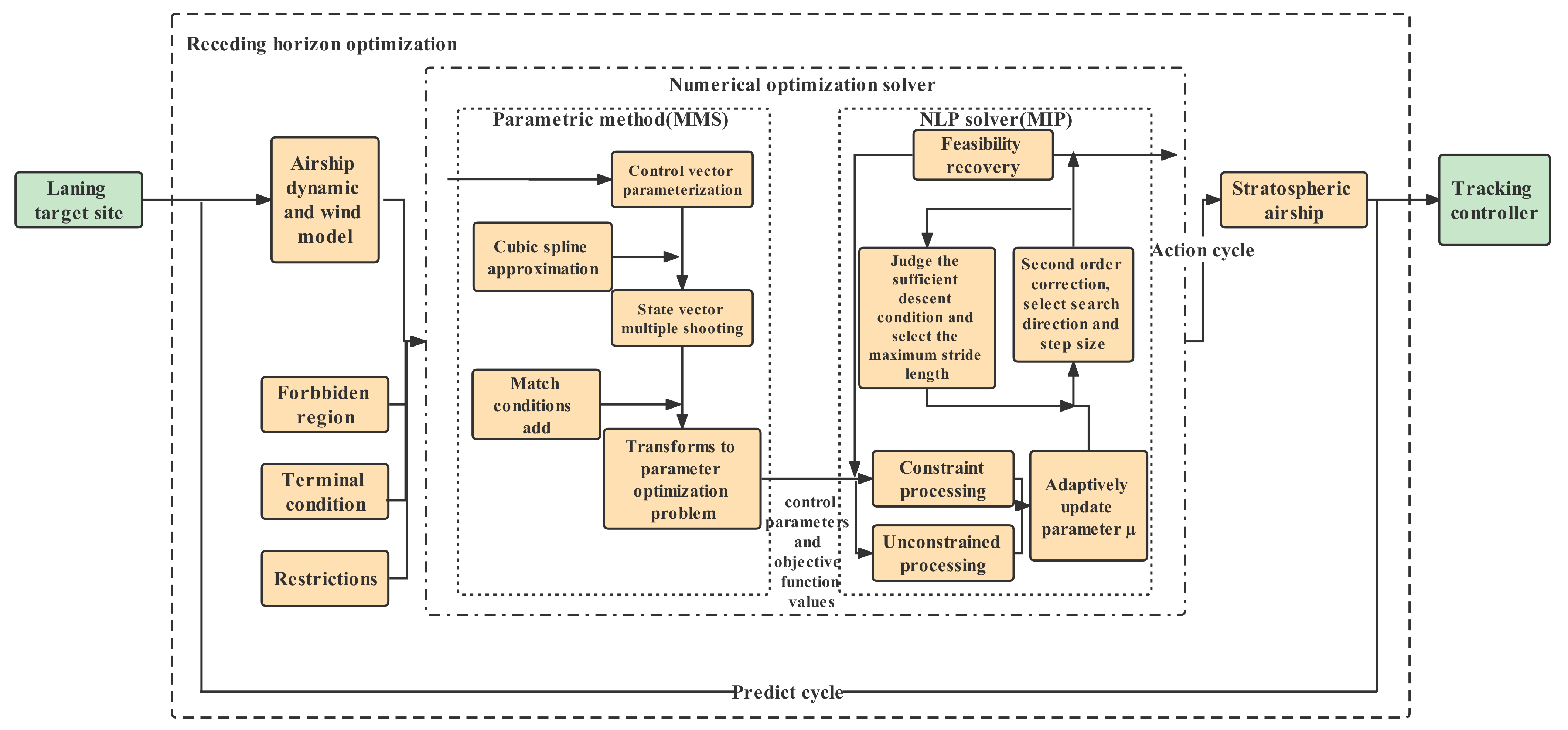
• The trajectory generation of a stratospheric airship was solved by converting the boundary value problem into parameter optimization according to the modified multiple shooting method, and transforming the inequality constraint into a penalty function by using the modified interior point method.
• An adaptive gradient descent regulator was used to reduce the influence on the optimization result due to different selections of the initial search point, and the convergence was made faster and more stable.

The section structure of this paper is as follows. The dynamic model and kinematic model of stratosphere airships are established in Section 2. The wind field model is also denoted. Then, numerical solution methods are proposed in Section 3. In Section 4, two numerical optimization results are carried out, which are the influence of wind effects on trajectory generation and the comparison between different methods.

2. Dynamic Model and Problem Formulation

The six-degrees-of-freedom (6-DOF) dynamics and kinematics equations of a stratospheric airship are introduced in this section [26]. The reference frames of an airship, including the earth reference frame (ERF), the body reference frame (BRF) and the path parallel frame (PPF), are defined in Figure 2, based on Zhou’s work [27]. $\mathbf{P},\Omega$ denote the relative position and the attitude of airships, respectively, and $\mathbf{V},\mathbf{W}$$v,w$ are the velocity and the angular velocity in the body reference frame of airships, respectively.

Define

$$\zeta =\left[\begin{array}{c}\mathbf{P}\hfill \\ \Omega \hfill \end{array}\right],\eta =\left[\begin{array}{c}\mathbf{V}\\ \mathbf{W}\end{array}\right]$$

(1)

$${\left[\begin{array}{c}\mathbf{P}\\ \Omega \\ \mathbf{V}\\ \mathbf{W}\end{array}\right]}^{\mathrm{T}}=\left[\begin{array}{cccc}{x}_{\mathrm{g}}& \varphi & u& p\\ y_{\mathrm{g}}& \theta & v& q\\ z_{\mathrm{g}}& \psi & w& r\end{array}\right]$$

(2)

2.1. Kinematics and Dynamics Equations of the Stratospheric Airship

Consider the kinematics of airships in the following form:

$$\dot{\mathbf{P}}={\mathbf{R}}_{\mathrm{I}}^{\mathrm{B}}\mathbf{V}$$

(3)

$$\dot{\Omega }=\Phi \mathbf{W}$$

(4)

where ${\mathbf{R}}_{\mathrm{I}}^{\mathrm{B}}$, $\Phi$ are the direction cosine transformation matrix and the angular transformation matrix from BRF to ERF, respectively. The velocity and the angular velocity can be converted from BRF to ERF. Both of them can be considered in the following Equations (5) and (6).

$${\mathbf{R}}_{\mathrm{I}}^{\mathrm{B}}=\left[\begin{array}{ccc}cos\psi cos\theta & cos\psi sin\theta sin\varphi -sin\psi cos\varphi & cos\psi sin\theta cos\varphi +sin\psi sin\varphi \\ sin\psi cos\theta & sin\psi sin\theta sin\varphi +cos\psi cos\varphi & sin\psi sin\theta cos\varphi -cos\psi sin\varphi \\ -sin\theta & cos\theta sin\varphi & cos\theta cos\varphi \end{array}\right]$$

(5)

$$\Phi =\left[\begin{array}{ccc}1& sin\varphi tan\theta & cos\varphi tan\theta \\ 0& cos\varphi & -sin\varphi \\ 0& sin\varphi sec\theta & cos\varphi sec\theta \end{array}\right]$$

(6)

The dynamic model can be denoted as

$$\mathbf{M}·\left[\begin{array}{c}\mathbf{V}\\ \mathbf{W}\end{array}\right]={\mathbf{F}}_{\mathrm{GB}}+{\mathbf{F}}_{\mathrm{I}}+{\mathbf{F}}_{\mathrm{A}}+{\mathbf{F}}_{\mathrm{T}}$$

(7)

where $\mathbf{M}$ represents the inertia matrix, denoted by Equation (8), where m is the total mass of the airship, $m_{\mathrm{i}\mathrm{i}},i=1\dots 6$ represents the additional mass, $I_{\mathrm{x}},I_{\mathrm{y}},I_{\mathrm{z}},I_{\mathrm{x}\mathrm{y}},I_{\mathrm{x}\mathrm{z}}$ and $I_{\mathrm{y}\mathrm{z}}$ stand for the inertia and $\left[x_{\mathrm{G}},y_{\mathrm{G}},z_{\mathrm{G}}\right]$ represents the center of airship gravity.

$$\mathbf{M}=\left[\begin{array}{cccccc}m+m_{11}& 0& 0& 0& m{z}_{\mathrm{G}}& -m{y}_{\mathrm{G}}\\ 0& m+m_{22}& 0& -m{z}_{\mathrm{G}}& 0& m_{26}+m{x}_{\mathrm{G}}\\ 0& 0& m+m_{33}& m{y}_{\mathrm{G}}& m_{35}-m{x}_{\mathrm{G}}& 0\\ 0& -m{z}_{\mathrm{G}}& m{y}_{\mathrm{G}}& I_{\mathrm{x}}+m_{44}& -I_{\mathrm{x}\mathrm{y}}& -I_{\mathrm{x}\mathrm{z}}\\ m{z}_{\mathrm{G}}& 0& m_{53}-m{x}_{\mathrm{G}}& -I_{\mathrm{x}\mathrm{y}}& I_{\mathrm{y}}+m_{55}& -I_{\mathrm{y}\mathrm{z}}\\ -m{y}_{\mathrm{G}}& m_{62}+m{x}_{\mathrm{G}}& 0& -I_{\mathrm{x}\mathrm{z}}& -I_{\mathrm{y}\mathrm{z}}& I_{\mathrm{z}}+m_{66}\end{array}\right]$$

(8)

where ${\mathbf{F}}_{\mathrm{GB}}$ is the resultant force of gravity and buoyancy, ${\mathbf{F}}_{\mathrm{A}}$, ${\mathbf{F}}_{\mathrm{I}}$ and ${\mathbf{F}}_{\mathrm{T}}$ are the aerodynamic force, inertial force, Coriolis force and the propeller force, respectively. The detailed expressions of these matrics mentioned above are given in [28].

Remark 1.

From the system input as the propeller force ${\mathbf{F}}_{\mathrm{T}}$, it is clear that the stratospheric airship is under-actuated and lateral motion cannot be controlled directly.

Assumption 1.

It is known from [29] that the rolling angle ϕ of the airship is uncontrollable, which is set to zero in three-dimensional trajectory optimization.

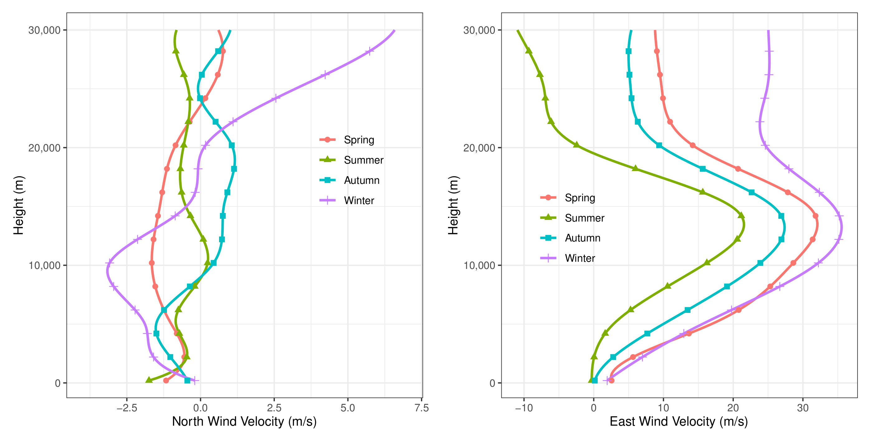
2.2. Wind Field Models

Based on Azinheira’s work [30] and Sarma’s work [31], it is known that the horizontal wind movement is considered to be the steady wind with the disturbance of gust, which can affect the accuracy of the trajectory during the airship return phase. The amplitude of the wind varying with altitude is called the vertical wind shear, affecting the flight safety.

The wind profile generated by HWM14 [32] was used in the position of ${85}^{\circ }\mathrm{E}$, ${42}^{\circ }\mathrm{N}$, which is the outdoor experiment site. Horizontal wind velocities in different seasons are shown in Figure 3. The horizontal wind in summer and autumn is obviously weaker than that in winter and spring, which is also the reason why it is better to select the outdoor experiment in the summer. At an altitude of approximately 19.5 km, there will be an area with nearly zero wind velocity, which is called the quasi-zero wind layer, and is the frequently selected stationary point.

The summer wind field was selected as the numerical experiment environment as shown in Figure 4. Equation (9) denotes the fitting relationship between wind velocity and altitude.

$$\begin{array}{c}\hfill w_{\mathrm{E}}\left(\overline{h}\right)=\sum _{\mathrm{i}=0}^7{p}_{(8-\mathrm{i})\mathrm{e}}{\overline{h}}^{\mathrm{i}},\\ \hfill w_{\mathrm{N}}\left(\overline{h}\right)=\sum _{\mathrm{i}=0}^7{p}_{(8-\mathrm{i})\mathrm{e}}{\overline{h}}^{\mathrm{i}}\end{array}$$

(9)

where $w_{\mathrm{E}}$ and $w_{\mathrm{N}}$ are the east wind speed and north wind speed, respectively. In order to keep the data at the 0 mean value, $\overline{h}=\left(h-{\mu }_{\mathrm{d}}\right)/{\sigma }_{\mathrm{d}}$ is used as the independent variable for fitting, and ${\mu }_{\mathrm{d}}$ = 15,000 m and ${\sigma }_{\mathrm{d}}=8660.4$ m. $p_{\mathrm{i}\mathrm{e}}$ and $p_{\mathrm{i}\mathrm{n}}(i=1\sim 8)$ are the fitting coefficients, respectively, and the values are summarized as follows:

$$\begin{array}{cc}\hfill {\mathbf{p}}_{\mathrm{e}}& ={[0.971,9.714,35.940,53.170,4.215,-56.070,-20.270,19.610]}^{\mathrm{T}},\hfill \\ \hfill {\mathbf{p}}_{\mathrm{n}}& ={[0.193,-2.959,-9.812,-4.780,6.499,2.615,-1.835,-0.470]}^{\mathrm{T}}\hfill \end{array}$$

(10)

The acceleration of wind is derived in Equation (11).

$$\begin{array}{cc}\hfill \dot{\mathbf{w}}& =\dot{{\mathbf{R}}_{\mathrm{s}}}{\mathbf{w}}_{\mathrm{i}}+{\mathbf{R}}_{\mathrm{s}}{\dot{\mathbf{w}}}_{\mathrm{i}}\hfill \\ \hfill & ={\mathbf{R}}_{\mathrm{s}}{\dot{\mathbf{w}}}_{\mathrm{i}}-\Omega ·{\mathbf{R}}_{\mathrm{s}}{\mathbf{w}}_{\mathrm{i}}\hfill \\ \hfill & ={\mathbf{R}}_{\mathrm{s}}{\dot{\mathbf{w}}}_{\mathrm{i}}-\Omega ·\mathbf{w}\hfill \end{array}$$

(11)

where ${\mathbf{w}}_{\mathrm{i}}$ is the wind speed in ERF, ${\mathbf{R}}_{\mathrm{s}}$ is the transform matrix from ERF to BRF and $\Omega$ is the angular velocity of the airship in BRF. The force generated by the wind is expressed by Equation (12).

$${\mathbf{F}}_{\mathrm{w}}={\mathbf{M}}_{\mathrm{Bw}}\dot{\mathbf{w}}+\Omega ·{\mathbf{M}}_{\mathrm{Bw}}\mathbf{w}$$

(12)

where ${\mathbf{M}}_{\mathrm{Bw}}=\left[\begin{array}{cc}{\mathbf{m}}_{\mathrm{Bw}}& {\mathbf{0}}_{3\times 3}\\ {\mathbf{0}}_{3\times 3}& {\mathbf{J}}_{\mathrm{B}\mathrm{w}}\end{array}\right]=\left[\begin{array}{cc}{\mathbf{m}}_{\mathrm{B}}{\mathbf{I}}_3+{\mathbf{M}}_{\mathrm{v}}& {\mathbf{0}}_{3\times 3}\\ {\mathbf{0}}_{3\times 3}& {\mathbf{J}}_{\mathrm{B}}+{\mathbf{J}}_{\mathrm{v}}\end{array}\right]$, ${\mathbf{m}}_{\mathrm{B}}$ is the mass of the airship and ${\mathbf{J}}_{\mathrm{B}}$ is the moment of buoyancy generated by the airship. ${\mathbf{M}}_{\mathrm{v}}$ and ${\mathbf{J}}_{\mathrm{v}}$ are the added mass and added moment of the airship, respectively. The effect of vertical wind shear is represented by Equation (13) with altitude changing.

$$\begin{array}{cc}\hfill {\mathbf{F}}_{\mathrm{w}}\left(\mathbf{h}\right)& ={\mathbf{M}}_{\mathrm{B}\mathrm{w}}{\mathbf{R}}_{\mathrm{s}}{\dot{\mathbf{w}}}_{\mathrm{i}}\left(\mathbf{h}\right)-{\mathbf{M}}_{\mathrm{B}\mathrm{w}}\Omega ·\mathbf{w}\left(\mathbf{h}\right)+\Omega ·{\mathbf{M}}_{\mathrm{B}\mathrm{w}}\mathbf{w}\left(\mathbf{h}\right)\hfill \\ \hfill & ={\mathbf{M}}_{\mathrm{B}\mathrm{w}}{\mathbf{R}}_{\mathrm{s}}{\dot{\mathbf{w}}}_{\mathrm{i}}\left(\mathbf{h}\right)-{\mathbf{M}}_{\mathrm{B}\mathrm{w}}\Omega ·{\mathbf{R}}_{\mathrm{s}}^{-1}{\mathbf{w}}_{\mathrm{i}}\left(\mathbf{h}\right)+\Omega ·{\mathbf{M}}_{\mathrm{B}\mathrm{w}}{\mathbf{R}}_{\mathrm{s}}^{-1}{\mathbf{w}}_{\mathrm{i}}\left(\mathbf{h}\right)\hfill \end{array}$$

(13)

Assumption 2.

Based on the steady horizontal wind, the angular and vertical velocity of the wind are not considered.

3. Optimal Numerical Solution

Under the description of the above models, the receding horizon trajectory optimization model was established, and an objective function was designed by using the terminal cost and process cost to characterize the time and energy consumption of the trajectory. In the case of that, the path constraint, differential constraint and boundary constraints are aimed at expressing the forbidden region and the dynamics of the airship, as well as the environment model and target point, respectively. In this section, the trajectory optimization problem is transformed into a nonlinear programming problem (NLP) by using a parametric method to generate a smooth and effective trajectory. A flowchart of this process is shown in Figure 5.

3.1. Conversion of Bolza Problem

The airship receding horizon trajectory optimization problem is solved by converting it to an initial value problem on each optimization period, which has the Bolza form as Equation (14).

$$\begin{array}{cc}\hfill & \underset{\zeta (·),\eta (·)}{min}J={\int }_{t_0}^{t_{\mathrm{f}}}P(t,\zeta \left(t\right),\eta \left(t\right),{\mathbf{u}}_{\mathrm{t}};\mathbf{s})\mathrm{d}t+R\left(t_{\mathrm{f}},\zeta \left({\mathit{t}}_{\mathrm{f}}\right),\eta \left({\mathit{t}}_{\mathrm{f}}\right)\right)\hfill \\ \hfill & s.t.\left\{\begin{array}{c}{\left[\begin{array}{cc}\zeta \left({\mathit{t}}_0\right)& \eta \left({\mathit{t}}_0\right)\end{array}\right]}^T-{\widehat{\mathbf{x}}}_0=\mathbf{0}\hfill \\ l\left(t,\dot{\zeta }\left(\mathit{t}\right),\dot{\eta }\left(\mathit{t}\right),\zeta \left(\mathit{t}\right),\eta \left(\mathit{t}\right),{\mathbf{u}}_{\mathrm{t}};\mathbf{s}\right)=0,\forall t\in \left[t_0,t_{\mathrm{f}}\right]\hfill \\ g\left(\zeta \left(\mathit{t}\right),\eta \left(\mathit{t}\right);\mathbf{s}\right)\le 0,\forall t\in \left[t_0,t_{\mathrm{f}}\right]\hfill \\ h\left(\zeta \left({\mathit{t}}_{\mathrm{f}}\right),\eta \left({\mathit{t}}_{\mathrm{f}}\right);\mathbf{s}\right)=0\hfill \end{array}\right.\hfill \end{array}$$

(14)

where ${\left[\begin{array}{cc}\zeta & \eta \end{array}\right]}^T$ and ${\widehat{\mathbf{x}}}_0$ denote the state variables and the initial state value, respectively, and $\mathbf{s}$ is the combined parameter variable. P and R are the process energy and terminal time consuming object, respectively. l, g and h represent the Lipschitz continuous function, path constraint and terminal boundary constraint of the airship, respectively.

$$u_{\mathrm{i}}^{\mathrm{k}}\left(t\right)={\mathbf{D}}_{\mathrm{i}}\left[\begin{array}{c}{F}_{\mathrm{Ti}}^{\mathrm{k}}\left(t\right)sin{\mu }_{\mathrm{i}}^{\mathrm{k}}\left(t\right)\\ F_{\mathrm{Ti}}^{\mathrm{k}}\left(t\right)cos{\mu }_{\mathrm{i}}^{\mathrm{k}}\left(t\right)\end{array}\right]$$

(15)

The action horizon is divided into $I_{\mathrm{k}}:=\left[t_{\mathrm{k}-1},t_{\mathrm{k}}\right],(k=1,2,\dots ,N)$. $u_{\mathrm{i}}^{\mathrm{k}}\left(t\right)$, $F_{\mathrm{Ti}}^{\mathrm{k}}\left(t\right)$ and ${\mu }_{\mathrm{i}}^{\mathrm{k}}\left(t\right)$ are each control component, each thrust force and the force vector angles. ${\mathbf{D}}_{\mathrm{i}}$ is the input transformation in Equation (15), approximated as

$$u_{\mathrm{i}}^{\mathrm{k}}\left(t\right)\approx \sum _{\mathrm{ord}=1}^{\mathrm{M}+1}{\left[{\gamma }_{\mathrm{i},\mathrm{ord}}^{\mathrm{k}}\left(t\right)\right]}^{\mathrm{ord}}{\lambda }_{\mathrm{i},\mathrm{ord}}^{\mathrm{k}}$$

(16)

where ${\left[{\gamma }_{\mathrm{i},\mathrm{ord}}^{\mathrm{k}}\left(t\right)\right]}^{\mathrm{ord}}$, ${\lambda }_{\mathrm{i},\mathrm{ord}}^{\mathrm{k}}$, $ord$ are the basis function, linear combination coefficient and the order number of the basis function. Cubic spline approximation is selected as Equation (17).

$$\begin{array}{cc}\hfill u_{\mathrm{i}}^{\mathrm{k}}\left(t\right)& ={\dot{u_{\mathrm{i}}}}^{\mathrm{k}}\left(t_{\mathrm{k}-1}\right)\frac{{(t_{\mathrm{k}}-t)}^3}{6\tau }+{\dot{u_{\mathrm{i}}}}^{\mathrm{k}}\left(t_{\mathrm{k}}\right)\frac{{(t-t_{\mathrm{k}-1})}^3}{6\tau }\hfill \\ \hfill & +\frac{(t_{\mathrm{k}}-t)}{\tau }(u_{\mathrm{i}}^{\mathrm{k}}\left(t_{\mathrm{k}-1}\right)-\frac{{\dot{u_{\mathrm{i}}}}^{\mathrm{k}}\left(t_{\mathrm{k}-1}\right){\tau }^2}{6})+\frac{(t-t_{\mathrm{k}-1})}{\tau }(u_{\mathrm{i}}^{\mathrm{k}}\left(t_{\mathrm{k}}\right)-\frac{{\dot{u_{\mathrm{i}}}}^{\mathrm{k}}\left(t_{\mathrm{k}}\right){\tau }^2}{6}),\hfill \\ \hfill & k=1,2,\dots ,N\hfill \end{array}$$

(17)

where $\tau =t_{\mathrm{k}}-t_{\mathrm{k}-1}$ is the interval time. Thus, the control component is parameterized as ${\sigma }_{\mathrm{i}}^{\mathrm{k}}={\left[\begin{array}{cccc}{\dot{u_{\mathrm{i}}}}^{\mathrm{k}}\left(t_{\mathrm{k}-1}\right)& {\dot{u_{\mathrm{i}}}}^{\mathrm{k}}\left(t_{\mathrm{k}}\right)& {u_{\mathrm{i}}}^{\mathrm{k}}\left(t_{\mathrm{k}-1}\right)& {u_{\mathrm{i}}}^{\mathrm{k}}\left(t_{\mathrm{k}}\right)\end{array}\right]}^T$.

Remark 2.

Due to the the airship complex dynamic characteristics and non-directivity of the objective function, it is unrealistic to solve the problem by using the analytic method [33,34], namely, the method of finding extremum by a functional. Refs. [35,36,37] used piecewise constants or polynomials to discretize control variables and was not suitable for the smoothing input on the optimized object. In this paper, the start and end states of each time interval are substituted into a cubic spline approximation formula. Robust and gentle trajectories can be generated more quickly using this method.

The MMS method approximately transforms the boundary value problem (BVP) into an NLP problem by means of discretization as Equation (18).

$$\begin{array}{cc}\hfill & {\dot{\mathbf{x}}}_{\mathrm{k}}\left(\mathbf{t}\right)=l\left[{\sigma }_{\mathrm{k}},{\mathbf{x}}_{\mathrm{k}}\left(\mathbf{t}\right),t\right],t\in \left[t_{\mathrm{k}},t_{\mathrm{k}+1}\right],\hfill \\ \hfill & {\mathbf{x}}_{\mathrm{k}}\left({\mathbf{t}}_{\mathrm{k}}\right)={\chi }_{\mathrm{k}}\hfill \end{array}$$

(18)

where $\mathbf{x}\left(\mathbf{t}\right)=\left[\begin{array}{cccc}\dot{\zeta \left(\mathit{t}\right)}& \dot{\eta \left(\mathit{t}\right)}& \zeta \left(\mathit{t}\right)& \eta \left(\mathit{t}\right)\end{array}\right]$ is the state variables, and ${\chi }_{\mathrm{k}}={\mathbf{x}}^{\mathrm{k}}\left({\mathbf{t}}_0\right),(k=1,2,\dots ,N)$ is the initial value of the state vector in each sub-interval. In this way, the airship receding horizon trajectory optimization problem is transformed into a finite dimensional NLP problem to determine the control parameters ${\sigma }_{\mathrm{k}}$ and auxiliary parameters ${\chi }_{\mathrm{k}}$ as Equation (19).

$$\begin{array}{cc}\hfill & \underset{{\chi }_{\mathrm{k}},{\sigma }_{\mathrm{k}}}{min}J=\sum _{\mathrm{k}=1}^{\mathrm{N}}{\int }_{{\mathrm{t}}_{\mathrm{k}-1}}^{{\mathrm{t}}_{\mathrm{k}}}P\left[t,{\mathbf{x}}_{\mathrm{k}}\left(\mathbf{t}\right),{\sigma }_{\mathrm{k}}\right]dt+R\left[\mathbf{x}\left({\mathbf{t}}_{\mathrm{f}}\right)\right]\hfill \\ \hfill & s.t.\left\{\begin{array}{c}\dot{\mathbf{x}}\left(\mathbf{t}\right)=\sum _{\mathrm{k}=1}^{\mathrm{N}}l\left[t,{\mathbf{x}}_{\mathrm{k}}\left(\mathbf{t}\right),{\sigma }_{\mathrm{k}}\right]\hfill \\ {\mathbf{x}}_{\mathrm{k}}\left({\mathbf{t}}_{\mathrm{k}}\right)={\chi }_{\mathrm{k}}\hfill \\ {\mathbf{x}}_{\mathrm{k}}\left({\mathbf{t}}_{\mathrm{k}+1}\right)-{\chi }_{\mathrm{k}+1}=0\hfill \\ g\left(t,{\mathbf{x}}_{\mathrm{k}}\left(\mathbf{t}\right),{\sigma }_{\mathrm{k}}\right)\le 0\hfill \\ h\left(t,{\mathbf{x}}_{\mathrm{k}}\left(\mathbf{t}\right),{\sigma }_{\mathrm{k}}\right)=0\hfill \\ {\mathit{u}}_{\mathrm{L}}\le {\sigma }_{\mathrm{k}}\le {\mathit{u}}_{\mathrm{U}}\hfill \\ t_{\mathrm{k}-1}\le t\le t_{\mathrm{k}},k=1,2,\dots ,N\hfill \end{array}\right.\hfill \end{array}$$

(19)

where ${\mathit{u}}_{\mathrm{U}}$ and ${\mathit{u}}_{\mathrm{L}}$ are the upper and lower boundary values of control parameters, respectively.

In order to ensure the continuity of the state curve, the MMS method adds the matching condition as the equality constraint.

Remark 3.

The main direct methods are the orthogonal collocation method (OC) and multiple shooting method (MS). Because conjugate variables are difficult to express explicitly, it is difficult to deal with the complex structure and repeatable deployment of airships. The key toward parameterization is that the new cubic spline is used to replace the Runge–Kutta segment approximating method to generate a smooth and efficient trajectory.

3.2. Parameter Nonlinear Optimization

The MIP method was adopted to deal with the large-scale nonlinear optimization problem transformed by the MMS method. The general form of the optimization problem is as follows.

$$\begin{array}{cc}\hfill & \underset{\mathrm{x}\in {\mathrm{R}}^{\mathrm{n}}}{min}J=f\left(x\right)\hfill \\ \hfill //& s.t.\left\{\begin{array}{c}{g}_{\mathrm{i}}\left(x\right)\le 0,i=1,\cdots ,n\hfill \\ h_{\mathrm{j}}\left(x\right)=0,j=1,\cdots ,m\hfill \end{array}\right.\hfill \end{array}$$

(20)

Inequality constraints are transformed into a penalty object as Equation (21).

$$J=f\left(x\right)+\sum _{\mathrm{i}=1}^{\mathrm{n}}{B}_{-}\left(g_{\mathrm{i}}\left(x\right)\right)\mathrm{s}.\mathrm{t}.h_{\mathrm{j}}\left(x\right)=0$$

(21)

with $g_{\mathrm{i}}\left(x\right)\le 0,B_{-}\left(g_{\mathrm{i}}\left(x\right)\right)=0;g_{\mathrm{i}}\left(x\right)>0,B_{-}\left(g_{\mathrm{i}}\left(x\right)\right)=\infty$. $B_{-}\left(g_{\mathrm{i}}\left(x\right)\right)$ can be approximately replaced by a continuous function $\frac{1}{\mu }ln\left(g_{\mathrm{i}}\left(x\right)\right)$.

$$J=f\left(x\right)+\frac{1}{\mu }\sum _{\mathrm{i}=1}^{\mathrm{n}}ln\left(g_{\mathrm{i}}\left(x\right)\right)\mathrm{s}.\mathrm{t}.h_{\mathrm{j}}\left(x\right)=0$$

(22)

as $\mu$ tends to infinity, $\frac{1}{\mu }ln\left(g_{\mathrm{i}}\left(x\right)\right)$ tends to $B_{-}\left(g_{\mathrm{i}}\left(x\right)\right)$. The corresponding Lagrangian function is Equation (23).

$$L(x,u,\nu )=f\left(x\right)+\sum _{\mathrm{i}=1}^{\mathrm{n}}{u}_{\mathrm{i}}{g}_{\mathrm{i}}\left(x\right)+\sum _{\mathrm{j}=1}^{\mathrm{m}}{\nu }_{\mathrm{j}}{h}_{\mathrm{j}}\left(x\right).$$

(23)

Theorem 1.

Let the optimal value of the original problem be $Y^{*}$, and the optimal value of the dual problem be $R^{*}$. If $Y^{*}=R^{*}$, then there exists strong duality between the original problem and dual problem [38].

According to the strong duality of the primal problem and equivalent problem,

$$\begin{array}{cc}\hfill \nabla L(x,u,\nu )& =\nabla f\left(x\right)+\sum _{\mathrm{i}=1}^{\mathrm{n}}{u}_{\mathrm{i}}\nabla g_{\mathrm{i}}\left(x\right)+\sum _{\mathrm{j}=1}^{\mathrm{m}}{\nu }_{\mathrm{j}}\nabla h_{\mathrm{j}}\left(x\right)\hfill \\ & =\nabla f\left(x\right)+\sum _{\mathrm{i}=1}^{\mathrm{n}}\frac{1}{\mu g_{\mathrm{i}}\left(x\right)}\nabla g_{\mathrm{i}}\left(x\right)+\sum _{\mathrm{j}=1}^{\mathrm{m}}\frac{{\varsigma }_{\mathrm{j}}}{\mu }\nabla h_{\mathrm{j}}\left(x\right)=0.\hfill \end{array}$$

(24)

Theorem 2.

If $f\left(x\right),g_{\mathrm{i}}\left(x\right),h_{\mathrm{j}}\left(x\right)$ are differentiable, let $x^{*}$ be the optimal solution to the original optimization problem, and $(u_{\mathrm{i}}^{*},{\nu }_{\mathrm{j}}^{*})$ be the optimal solution of the dual problem. The strong duality is satisfied. Then, $\nabla f\left(x^{*}\right)+{\sum }_{\mathrm{i}=1}^{\mathrm{n}}{u}_{\mathrm{i}}^{*}\nabla g_{\mathrm{i}}\left(x^{*}\right)+{\sum }_{\mathrm{i}=1}^{\mathrm{m}}{\nu }_{\mathrm{j}}^{*}\nabla h_{\mathrm{j}}\left(x^{*}\right)=0$, where

$$\begin{array}{cc}\hfill g_{\mathrm{i}}\left(x^{*}\right)& \le 0,i=1,\cdots ,n\hfill \\ \hfill h_{\mathrm{j}}\left(x^{*}\right)& =0,j=1,\cdots ,m\hfill \\ \hfill u_{\mathrm{i}}^{*}& \ge 0,i=1,\cdots ,n\hfill \\ \hfill u_{\mathrm{i}}^{*}{g}_{\mathrm{i}}\left(x^{*}\right)& =0,i=1,\cdots ,n.\hfill \end{array}$$

(25)

The optimal solution of the original optimization problem is $p^{*}$; then,

$$\begin{array}{cc}\hfill p^{*}& \le L\left(x^{*}\left(t\right),u^{*}\left(t\right),{\nu }^{*}\left(t\right)\right)\hfill \\ \hfill & =f\left(x^{*}\left(t\right)\right)+\sum _{\mathrm{i}=1}^{\mathrm{n}}{u}_{\mathrm{i}}^{*}\left(t\right)g_{\mathrm{i}}\left(x^{*}\left(t\right)\right)+\sum _{\mathrm{j}=1}^{\mathrm{m}}{\nu }_{\mathrm{j}}^{*}\left(t\right)h_{\mathrm{j}}\left(x^{*}\left(t\right)\right)\hfill \\ \hfill & =f\left(x^{*}\left(t\right)\right)+\sum _{\mathrm{i}=1}^{\mathrm{n}}\left(\frac{1}{\mu g_{\mathrm{i}}\left(x^{*}\left(t\right)\right)}{g}_{\mathrm{i}}\left(x^{*}\left(t\right)\right)\right)+\sum _{\mathrm{j}=1}^{\mathrm{m}}{\nu }_{\mathrm{j}}^{*}\left(t\right)h_{\mathrm{j}}\left(x^{*}\left(t\right)\right)\hfill \\ \hfill & =f\left(x^{*}\left(t\right)\right)-\frac{n}{\mu }.\hfill \end{array}$$

(26)

The new $\mu$ parameter is obtained from

$${\mu }_{\mathrm{i}+1}=min\left\{\frac{n}{{ϵ}_{\mathrm{tol}}},max\left\{{\kappa }_{\mu }{\mu }_i,{\mu }_i^{{\theta }_{\mu }}\right\}\right\}$$

(27)

Thus, when $\mu \to \infty$, $f\left(x^{*}\left(t\right)\right)\to p^{*}$ is the optimal solution of the original problem.

The MIP method transforms the inequality constraint problem into an unconstrained optimization problem. Finally, the descending direction of the iteration point is obtained by the Newton iteration method, etc.

Remark 4.

The basic idea of the MIP method is to construct an interior penalty function so that the iteration point is always able to move in the feasible region constituted by various constraints [39,40]. However, it is a key point to choose the appropriate interior point as the initial point in the feasible region. In this paper, the iteration value of the barrier parameters μ can be adaptive-obtained.

4. Optimal Flight Trajectory Result

In this section, the summer wind field is considered as the environmental factor, because the horizontal wind speed in summer is relatively lower. The main parameters of airships [41] are able to be seen in

Table 1. Airship model parameters.

Airship Parameters	Value
Length, $\mathrm{m}$	$25.0$
Maximum diameter, $\mathrm{m}$	$7.576$
Fineness ratio of the hull	$3.3$
Volume of the hull, ${\mathrm{m}}^3$	$750.0$
Surface area, ${\mathrm{m}}^2$	$480.388$
Location of maximum diameter, $\mathrm{m}$	$9.840$
Moment center, ${\mathrm{m}}^2$	$12.001$
Reference area, ${\mathrm{m}}^2$	$82.544$
Reference length, $\mathrm{m}$	$25.0$
Volume Reynolds number	1.8–9.3 $\times {10}^6$

. There are two numerical optimization solution analyses, which are, respectively, the analysis of the influence of the wind field on the optimization and the comparison of results between different methods.

Receding horizon optimization was used to divide the whole planning horizon into several moments at equal intervals, and the information of the future period and real-time detection was used to carry out online planning. Cost function optimization was carried out within each prediction cycle, and optimization results were input within the input cycle. Relevant parameters of the optimal numerical experiment are listed in the

Table 2. Receding horizon parameters.

Receding Horizon Parameters	Value
Sampling interval, $\mathrm{s}$	$0.5$
Predict cycle	600
Input interval, $\mathrm{s}$	$0.2$
Action cycle	500

.

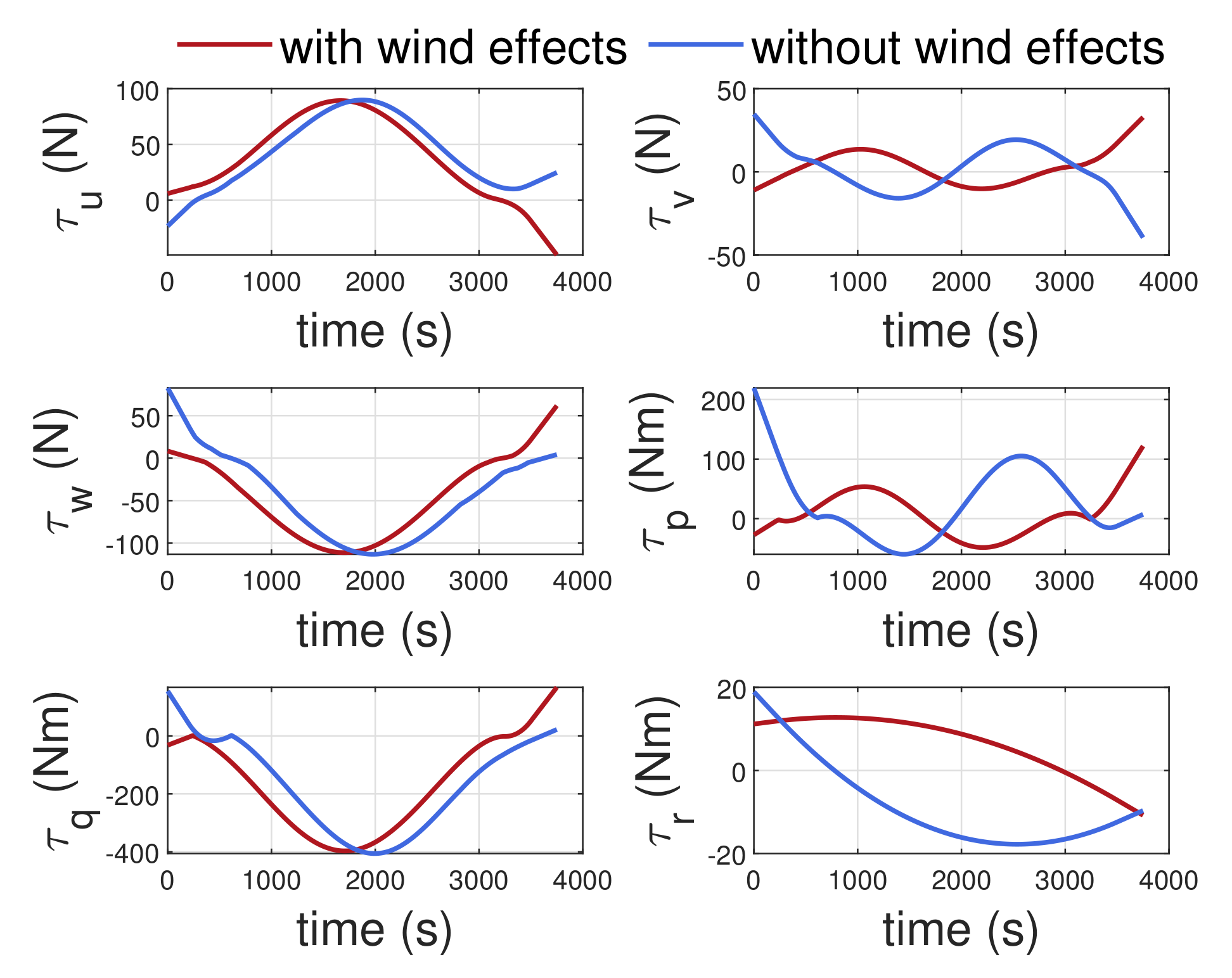
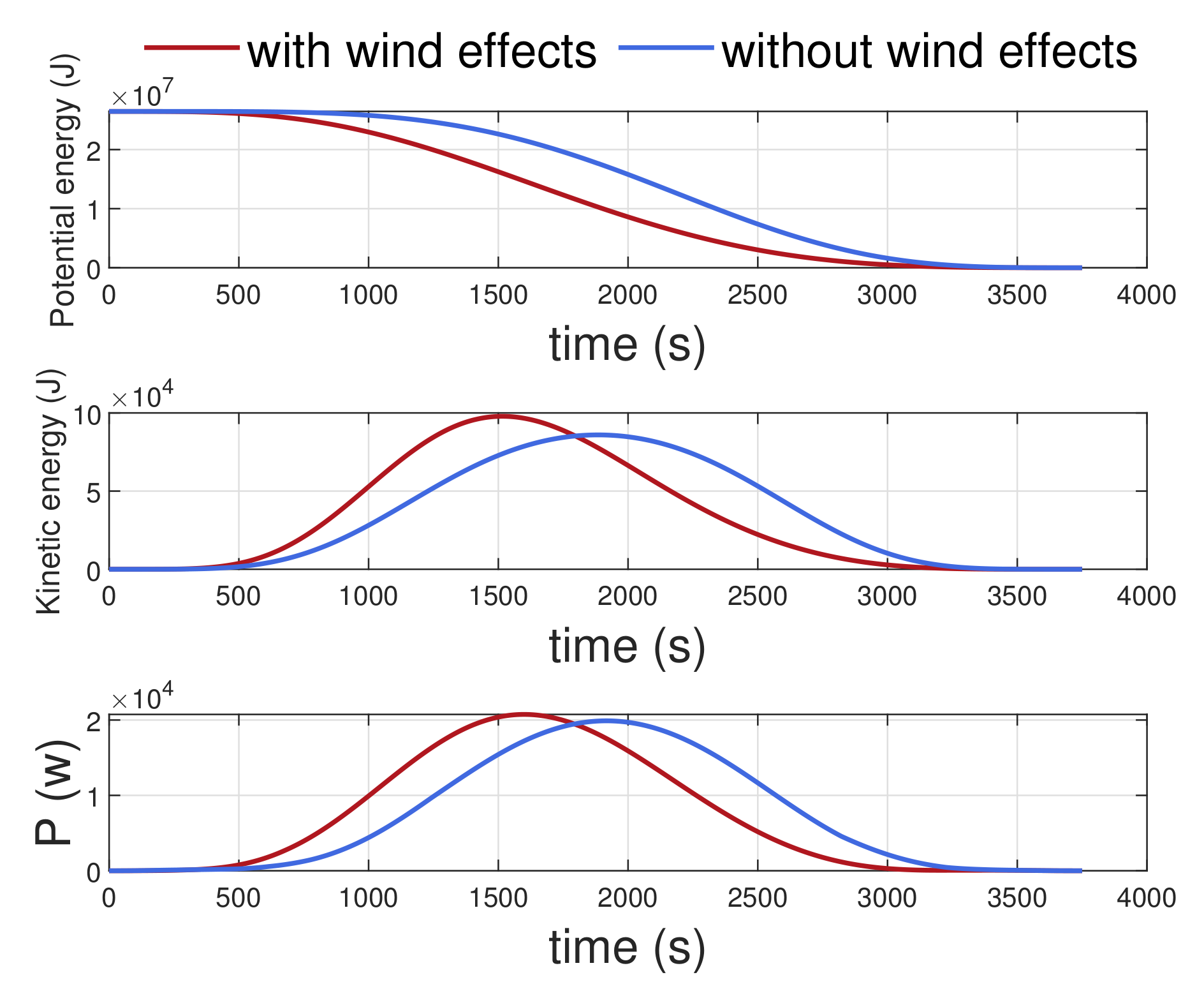
4.1. Optimization Effect under Wind Field

After ballonet valves are opened and the lighter-than-air gas is released, the low-altitude return starts to be executed. The flight path is set to return to the predetermined landing site from the stationary position, and the airship cannot pass through the forbidden regions with areas 15.90 ${\mathrm{km}}^2$, 7.07 ${\mathrm{km}}^2$ and 12.57 ${\mathrm{km}}^2$ during the flight (cylindrical areas shown in Figure 6). In the process of trajectory optimization, the upper limit of the linear velocity of the airship $\left|u\right|$ is specified as 15 $\mathrm{m}/\mathrm{s}$ and the upper limit of the descent speed $\left|w\right|$ is specified as 3 $\mathrm{m}/\mathrm{s}$. The initial position is (0.48,0.6,3) km and the terminal position is (22,22,0) km.

Two cases were compared to reflect the influence of wind on the optimized trajectory. In the first case, wind effects were considered. In the second case, wind effects were not added. The three-dimensional optimization schematic comparison of two cases is expressed as Figure 6 and Figure 7.

The position and attitude changes during the airship’s return phase in the two cases are shown in Figure 8. Because the east wind direction is y axis forward, the north wind direction is x axis negative. Therefore, at position y, due to the influence of wind, the speed will be increased to reach the target landing site in advance, whereas, at position x, the speed will be reduced to delay the arrival of the target landing site. If there is no wind, the optimized trajectory is through the first and second forbidden region to reach the landing site to reduce mileage. However, with wind effects, such a trajectory is not feasible for airship dynamics. Thus, the airship will initially start at a yaw angle $\psi$ of 62 $\mathrm{deg}$ to gradually reduce the yaw angle $\psi$ to circumnavigate the forbidden region and eventually arrive at the landing site.

The comparison of horizontal velocity and the yaw angle velocity $\left|r\right|$ during the airship’s return phase is shown in Figure 9 and Figure 10. The capacity of the airship angular velocity is of great significance for airship structural stability and stable operation, and represents the attitude change rate. The upper limit of the yaw angle velocity of the airship $\left|\psi \right|$ is specified as 0.05 $\mathrm{deg}/\mathrm{s}$. With wind effects, the yaw angle velocity r will decrease and then increase reversely. When t = 2500 $\mathrm{s}$, r will decrease again. Without the influence of the wind field, r will decrease the entire time until t = 3000 $\mathrm{s}$, and r will increase in reverse.

The comparison of energy and propulsion system power is shown in Figure 11. As can be seen from the variation in kinetic energy and potential energy during the airship’s return phase, wind will increase the amplitude of the kinetic energy change, but the power accumulation of the propulsion system does not increase significantly because the airship is in a downwind state. In general, wind will affect the attitude change and planning strategy of airships, and the optimized trajectory needs to avoid the drastic fluctuation in attitude to ensure the flight safety of the airship.

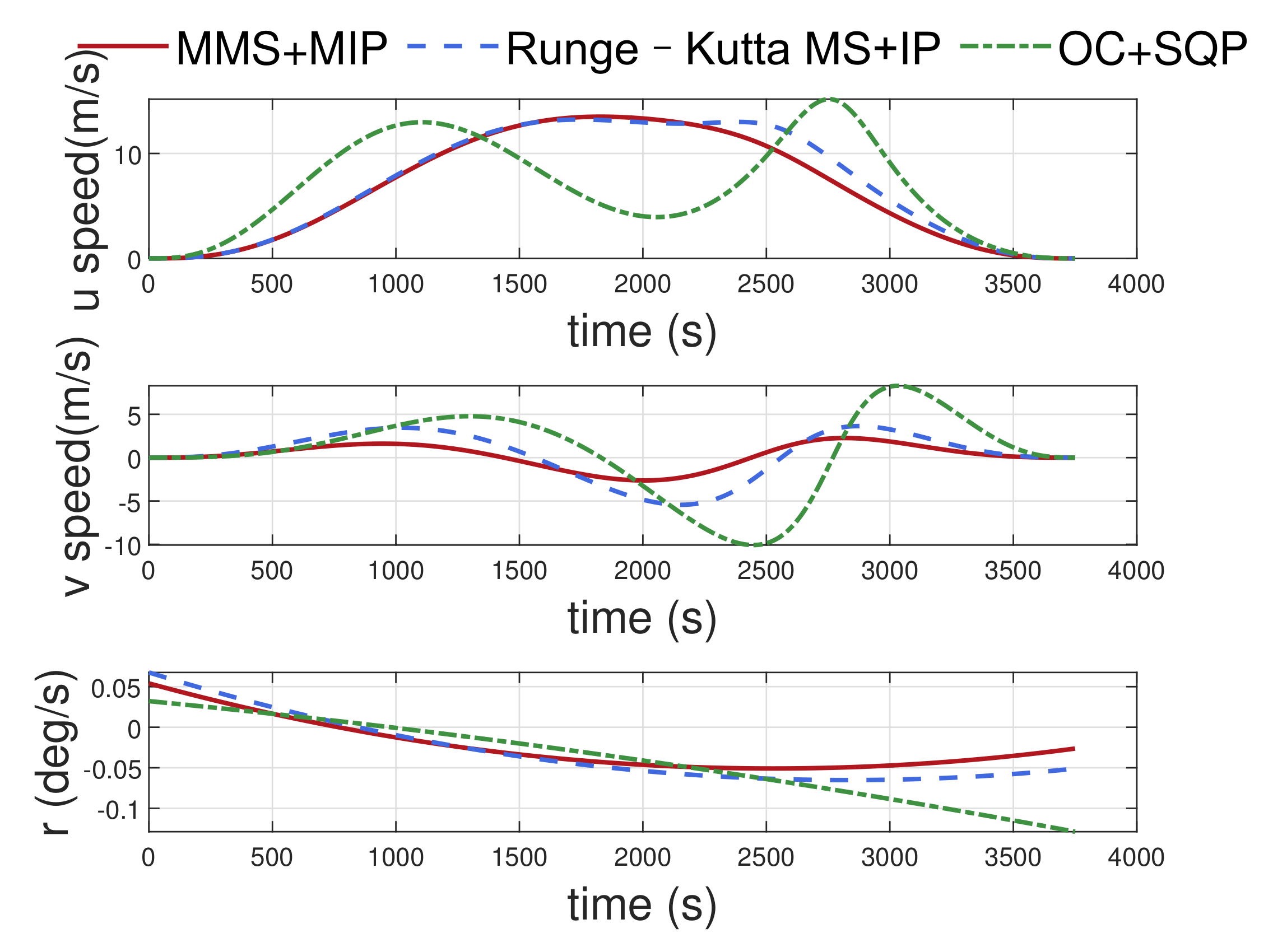
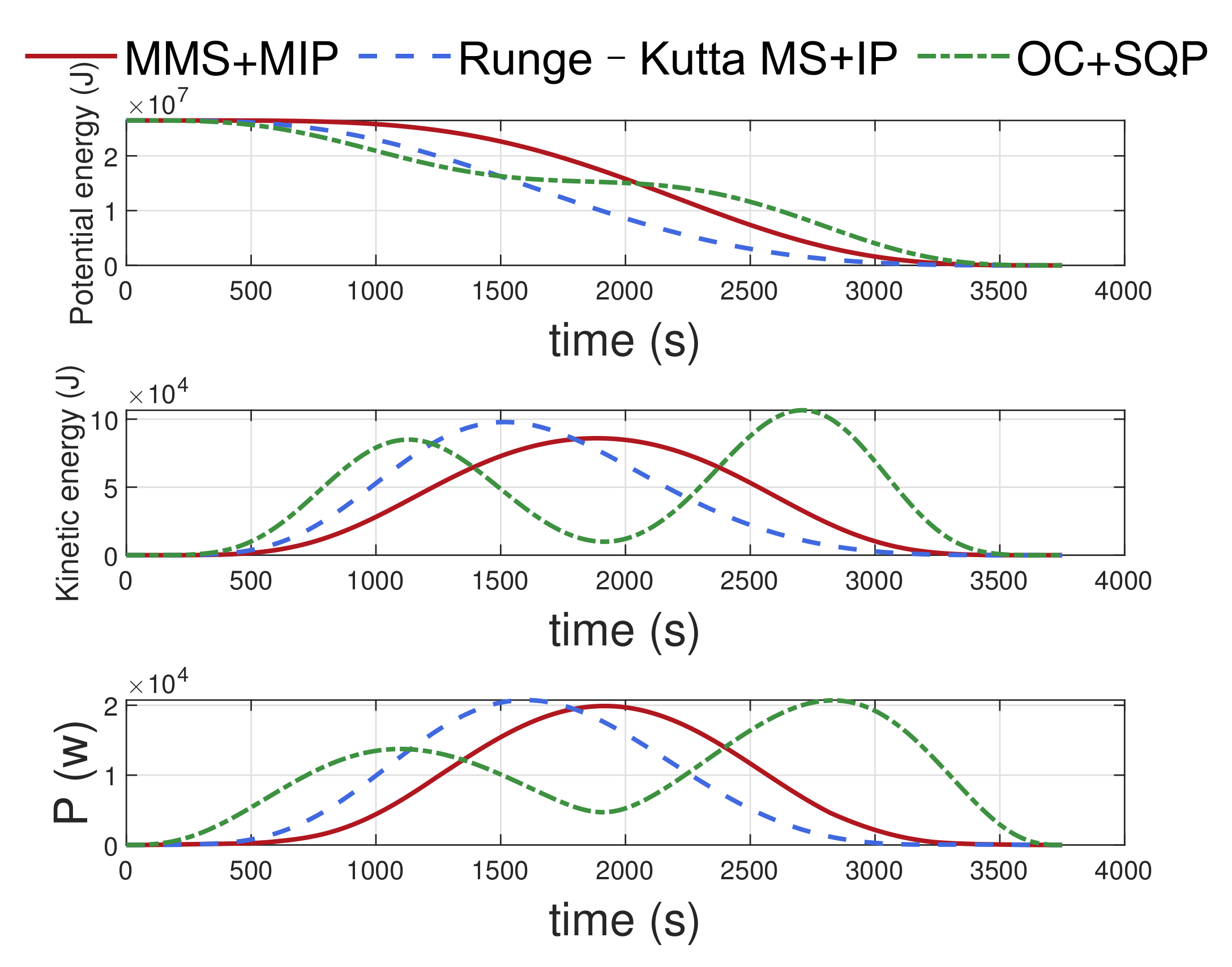
4.2. Comparison between Results of Different Methods

The stratospheric airship is a large inertia aircraft with a complex structure, so its state cannot be changed quickly. Therefore, it is very important to select a numerical solution method that can deal with a complex dynamics system and generate an efficient and smooth trajectory. The trajectory optimization of complex systems was firstly transformed into an NLP problem by a parameterized method, in which, the direct methods of the MS method and OC method were mainly used.

The OC method does not need numerical integration and has a high solving efficiency. A small number of collocation points can achieve a high conversion efficiency. It is an extremely effective method with sequential quadratic programming (SQP) for aircraft trajectory optimization. However, its conjugate variable cannot be approximated explicitly, and a poor estimation of it has a great impact on mesh refinement and the sensitivity of optimization performance indexes. In Figure 12 and Figure 13, a comparison of optimization results of the MMS method with the MIP method, the MS method with the interior-point method (IP) and the OC method with the SQP method is shown.

Under the same receding horizon parameters, airship parameters, terminal conditions and path conditions, certain differences between the optimized trajectories appear. In the t = 2000 $\mathrm{s}$, the yaw angle $\psi$ under the OC method changed greatly, which brought a great challenge to the steering moment actuator of the airship. The reason for this is that it is difficult to estimate the conjugate variables reasonably.

The improvements to the modified method can be seen more clearly in Figure 14 and Figure 15. The modified method generates the best trajectory and reduces the mileage at the location. The speed of the airship can also be controlled to be smaller, with a reduction of 2 $\mathrm{m}/\mathrm{s}$ for u and v. In addition, the yaw angle velocity r decreases by 0.02 $\mathrm{deg}/\mathrm{s}$. Figure 16 shows the variation curves of the airship’s energy and propulsion system power for different methods. The smoothness and stability of the energy change of the MMS+MIP method can be seen from the changing trend of potential energy and kinetic energy. The power integral of the airship’s propulsion system represents the main energy consumption during the return phase, and large power variations are unacceptable for the airship’s propulsion system. The power integration area of the MMS+MIP method is also significantly smaller than that of other methods. The advantages and disadvantages of the MS method and OC method are shown in

Table 3. Advantages and disadvantages of MS method and OC method.

Method	Advantage	Disadvantage
MS method	The structure is simple and easy to implement, and the result is smooth and stable	The convergence domain is narrow and the time grid is evenly divided
OC method	High solving efficiency and high conversion efficiency	Conjugate variable cannot be approximated explicitly; high sensitivity of mesh refinement and optimization index

.

In general, by modifying the connection link of the MS method and improving the convergence speed of the interior point adaptively, this method is beneficial to the smooth trajectory generation of an airship with large inertia.

5. Conclusions

This paper is concerned with the receding horizon trajectory optimization method of a stratospheric airship in a low-altitude return phase. The limit range of state variables and control variables was set according to the wind field, path constraints and energy consumption. The boundary value problem was transformed into a multi initial value problem using the MMS method, and inequality constraints were transformed into penalty functions using the MIP method. Essentially, the idea is to ensure that the airship is able to reach a prescribed geometric terminal target state with minimum dynamic model inputs smoothly. In addition, an adaptive gradient descent regulator was used to make the optimization solution fast and robust.

In the future, the energy acquisition of solar energy will be added as an optimization condition, and a trajectory tracker will be designed for the generated trajectory. The real-time sensing model of the wind field is also expected to make the trajectory generation more accurate.

References

1. Tang, J.; Pu, S.; Yu, P.; Xie, W.; Li, Y.; Hu, B. Research on Trajectory Prediction of a High-Altitude Zero-Pressure Balloon System to Assist Rapid Recovery. Aerospace 2022, 9, 622. [Google Scholar] [CrossRef]
2. Wang, Y.; Zhou, W.; Luo, J.; Yan, H.; Pu, H.; Peng, Y. Reliable intelligent path following control for a robotic airship against sensor faults. IEEE/ASME Trans. Mechatron. 2019, 24, 2572–2582. [Google Scholar] [CrossRef]
3. Zhou, P.; Wang, Y.; Duan, D. Adaptive fault-tolerant directional control of an autonomous airship against actuator fault. In Proceedings of the 2016 35th Chinese Control Conference (CCC), IEEE, Chengdu, China, 27–29 July 2016; pp. 10538–10542. [Google Scholar]
4. Tang, J.; Xie, W.; Wang, X.; Chen, C. Simulation and Analysis of Fluid–Solid–Thermal Unidirectional Coupling of Near-Space Airship. Aerospace 2022, 9, 439. [Google Scholar] [CrossRef]
5. Wu, Y.; Wang, Q.; Duan, D.; Xie, W.; Wei, Y. Neuroadaptive output-feedback trajectory tracking control for a stratospheric airship with prescribed performance. Aeronaut. J. 2020, 124, 1568–1591. [Google Scholar] [CrossRef]
6. Tang, J.; Duan, D.; Xie, W. Shape Exploration and Multidisciplinary Optimization Method of Semirigid Nearing Space Airships. J. Aircr. 2022, 59, 946–963. [Google Scholar] [CrossRef]
7. Tang, J.; Xie, W.; Wang, X.; Chen, Y.; Wu, J. Study of the Mechanical Properties of Near-Space Airship Envelope Material Based on an Optimization Method. Aerospace 2022, 9, 655. [Google Scholar] [CrossRef]
8. Teng, Y.; Song, Y.; Tong, S.; Zhang, M. Acquisition Performance of Laser Communication System Based on Airship Platform. Acta Opt. Sin. 2018, 38, 0606005. [Google Scholar] [CrossRef]
9. Yu, Z.; Zhang, Y.; Jiang, B.; Su, C.Y.; Fu, J.; Jin, Y.; Chai, T. Distributed fractional-order intelligent adaptive fault-tolerant formation-containment control of two-layer networked unmanned airships for safe observation of a smart city. IEEE Trans. Cybern. 2021, 52, 9132–9144. [Google Scholar] [CrossRef]
10. Zhao, Z.; Dong, X.; Feng, J.; Liang, X.; Hu, C. A Simulating Method of Airship-Borne Polarimetric Weather Radar for Typhoon Observation. In Proceedings of the IGARSS 2020—2020 IEEE International Geoscience and Remote Sensing Symposium, IEEE, Waikoloa, HI, USA, 19–24 July 2020; pp. 5306–5309. [Google Scholar]
11. Tang, J.; Wang, X.; Duan, D.; Xie, W. Optimisation and analysis of efficiency for contra-rotating propellers for high-altitude airships. Aeronaut. J. 2019, 123, 706–726. [Google Scholar] [CrossRef]
12. Chu, X.; Lin, X.; Lan, W. Energy-optimal rectilinear trajectory for stratospheric airships in constant wind field. In Proceedings of the 2013 IEEE International Conference on Cyber Technology in Automation, Control and Intelligent Systems, IEEE, Nanjing, China, 26–29 May 2013; pp. 264–269. [Google Scholar]
13. Guo, X.; Zhu, M. Ascent trajectory optimization for stratospheric airship with thermal effects. Adv. Space Res. 2013, 52, 1097–1110. [Google Scholar] [CrossRef]
14. Zhu, B.J.; Yang, X.X.; Deng, X.L.; Ma, Z.Y.; Hou, Z.X.; Jia, G.W. Trajectory optimization and control of stratospheric airship in cruising. Proc. Inst. Mech. Eng. Part I J. Syst. Control. Eng. 2019, 233, 1329–1339. [Google Scholar] [CrossRef]
15. Mueller, J.; Zhao, Y.; Garrard, W. Sensitivity and solar power analysis of optimal trajectories for autonomous airships. In Proceedings of the AIAA Guidance, Navigation, and Control Conference, Chicago, IL, USA, 10–13 August 2009; p. 6014. [Google Scholar]
16. Zhang, L.; Li, J.; Jiang, Y.; Du, H.; Zhu, W.; Lv, M. Stratospheric airship endurance strategy analysis based on energy optimization. Aerosp. Sci. Technol. 2020, 100, 105794. [Google Scholar] [CrossRef]
17. Lee, S.; Bang, H. Three-dimensional ascent trajectory optimization for stratospheric airship platforms in the jet stream. J. Guid. Control. Dyn. 2007, 30, 1341–1351. [Google Scholar] [CrossRef]
18. Zhu, W.; Li, J.; Xu, Y. Optimum attitude planning of near-space solar powered airship. Aerosp. Sci. Technol. 2019, 84, 291–305. [Google Scholar] [CrossRef]
19. Wang, J.; Meng, X.; Li, C. Recovery trajectory optimization of the solar-powered stratospheric airship for the station-keeping mission. Acta Astronaut. 2021, 178, 159–177. [Google Scholar] [CrossRef]
20. Blouin, C.; Lanteigne, E.; Gueaieb, W. Trajectory optimization of a small airship in a moving fluid. Trans. Can. Soc. Mech. Eng. 2016, 40, 191–200. [Google Scholar] [CrossRef] [Green Version]
21. Das, T.; Mukherjee, R.; Cameron, J. Optimal trajectory planning for hot-air balloons in linear wind fields. J. Guid. Control. Dyn. 2003, 26, 416–424. [Google Scholar] [CrossRef] [Green Version]
22. Ceruti, A.; Marzocca, P. Heuristic optimization of Bezier curves based trajectories for unconventional airships docking. Aircr. Eng. Aerosp. Technol. 2017, 89, 76–86. [Google Scholar] [CrossRef]
23. Zhang, J.; Yang, X.; Deng, X.; Lin, H. Trajectory control method of stratospheric airships based on model predictive control in wind field. Proc. Inst. Mech. Eng. Part G J. Aerosp. Eng. 2019, 233, 418–425. [Google Scholar] [CrossRef]
24. Bestaoui, Y.; Kahale, E. Time optimal 3D trajectories for a lighter than air robot with second order constraints with a piecewise constant acceleration. J. Aerosp. Inf. Syst. 2013, 10, 155–171. [Google Scholar] [CrossRef]
25. Mueller, J.B.; Zhao, Y.J.; Garrard, W.L. Optimal ascent trajectories for stratospheric airships using wind energy. J. Guid. Control. Dyn. 2009, 32, 1232–1245. [Google Scholar] [CrossRef]
26. Liu, S.; Sang, Y.; Jin, H. Robust model predictive control for stratospheric airships using LPV design. Control. Eng. Pract. 2018, 81, 231–243. [Google Scholar] [CrossRef]
27. Zhou, W.X.; Xiao, C.; Zhou, P.F.; Duan, D.P. Spatial path following control of an autonomous underactuated airship. Int. J. Control. Autom. Syst. 2019, 17, 1726–1737. [Google Scholar] [CrossRef]
28. Chen, L.; Zhou, G.; Yan, X.; Duan, D. Composite control of stratospheric airships with moving masses. J. Aircr. 2012, 49, 794–801. [Google Scholar] [CrossRef]
29. Zheng, Z.; Zhu, M.; Shi, D.; Wu, Z. Hovering control for a stratospheric airship in unknown wind. In Proceedings of the AIAA Guidance, Navigation, and Control Conference, National Harbor, MA, USA, 13–17 January 2014; p. 0973. [Google Scholar]
30. Azinheira, J.R.; de Paiva, E.C.; Bueno, S.S. Influence of wind speed on airship dynamics. J. Guid. Control. Dyn. 2002, 25, 1116–1124. [Google Scholar] [CrossRef]
31. Sarma, A.; Hochstetler, R.; Wait, T. Optimization of airship routes for weather. In Proceedings of the 7th AIAA ATIO Conf, 2nd CEIAT Int’l Conf on Innov and Integr in Aero Sciences, 17th LTA Systems Tech Conf; followed by 2nd TEOS Forum, Belfast, Ireland, 18–20 September 2007; p. 7880. [Google Scholar]
32. Gul, B.; Ameen, M.A.; Verhulst, T.G. Correlation between foEs and zonal winds over Rome, Okinawa and Townsville using Horizontal Wind Model (HWM14) during solar cycle 22. Adv. Space Res. 2021, 68, 4658–4664. [Google Scholar] [CrossRef]
33. Athans, M.; Canon, M. On the fuel-optimal singular control of nonlinear second-order systems. IEEE Trans. Autom. Control 1964, 9, 360–370. [Google Scholar] [CrossRef]
34. Bongiorno, J. Minimum-energy control of a second-order nonlinear system. IEEE Trans. Autom. Control 1967, 12, 249–255. [Google Scholar] [CrossRef]
35. Diedam, H.; Sager, S. Global optimal control with the direct multiple shooting method. Optim. Control. Appl. Methods 2018, 39, 449–470. [Google Scholar] [CrossRef]
36. Greco, C.; Di Carlo, M.; Vasile, M.; Epenoy, R. Direct multiple shooting transcription with polynomial algebra for optimal control problems under uncertainty. Acta Astronaut. 2020, 170, 224–234. [Google Scholar] [CrossRef]
37. Chen, Y.; Scarabottolo, N.; Bruschetta, M.; Beghi, A. Efficient move blocking strategy for multiple shooting-based non-linear model predictive control. IET Control Theory Appl. 2020, 14, 343–351. [Google Scholar] [CrossRef] [Green Version]
38. Wächter, A.; Biegler, L.T. On the implementation of an interior-point filter line-search algorithm for large-scale nonlinear programming. Math. Program. 2006, 106, 25–57. [Google Scholar] [CrossRef]
39. Guo, C.; Li, D.; Zhang, G.; Ding, X.; Curtmola, R.; Borcea, C. Dynamic interior point method for vehicular traffic optimization. IEEE Trans. Veh. Technol. 2020, 69, 4855–4868. [Google Scholar] [CrossRef]
40. Jiang, H.; Kathuria, T.; Lee, Y.T.; Padmanabhan, S.; Song, Z. A faster interior point method for semidefinite programming. In Proceedings of the 2020 IEEE 61st Annual Symposium on Foundations of Computer Science (FOCS), IEEE, Durham, NC, USA, 16–19 November 2020; pp. 910–918. [Google Scholar]
41. Wang, X.L.; Fu, G.Y.; Duan, D.P.; Shan, X.X. Experimental investigations on aerodynamic characteristics of the ZHIYUAN-1 airship. J. Aircr. 2010, 47, 1463–1468. [Google Scholar] [CrossRef]
Figure 1. Flow chart of the airship descent process.
Aerospace 09 00670 g001
Figure 2. Reference frames of a stratospheric airship.
Aerospace 09 00670 g002
Figure 3. (left) North wind velocity. (right) East wind velocity.
Aerospace 09 00670 g003
Figure 4. North and east component of the wind velocity in summer.
Aerospace 09 00670 g004
Figure 5. Flow chart of receding horizon trajectory generation during the airship return phase.
Aerospace 09 00670 g005
Figure 6. Three-dimensional schematic diagram of optimized trajectory.
Aerospace 09 00670 g006
Figure 7. Top view of optimized trajectory.
Aerospace 09 00670 g007
Figure 8. Position, attitude and change rate of the airship.
Aerospace 09 00670 g008
Figure 9. Horizontal speed and yaw angle velocity of the airship.
Aerospace 09 00670 g009
Figure 10. Control forces and torques of the airship.
Aerospace 09 00670 g010
Figure 11. Energy and power changes during the airship’s return phase.
Aerospace 09 00670 g011
Figure 12. Three-dimensional schematic diagram of different methods.
Aerospace 09 00670 g012
Figure 13. Top view of optimized trajectories between different methods.
Aerospace 09 00670 g013
Figure 14. Position, attitude and change rate of the airship between different methods.
Aerospace 09 00670 g014
Figure 15. Horizontal speed and yaw angle velocity of the airship between different methods.
Aerospace 09 00670 g015
Figure 16. Energy and power changes between different methods.
Aerospace 09 00670 g016