AI-Based Exhaust Gas Temperature Prediction for Trustworthy Safety-Critical Applications

Abstract

Data-driven condition-based maintenance (CBM) and predictive maintenance (PdM) strategies have emerged over recent years and aim at minimizing the aviation maintenance costs and environmental impact by the diagnosis and prognosis of aircraft systems. As the use of data and relevant algorithms is essential to AI-based gas turbine diagnostics, there are different technical, operational, and regulatory challenges that need to be tackled in order for the aeronautical industry to be able to exploit their full potential. In this work, the machine learning (ML) method of the generalised additive model (GAM) is used in order to predict the evolution of an aero engine’s exhaust gas temperature (EGT). Three different continuous synthetic data sets developed by NASA are employed, known as New Commercial Modular Aero-Propulsion System Simulation (N-CMAPSS), with increasing complexity in engine deterioration. The results show that the GAM can be predict the evolution of the EGT with high accuracy when using several input features that resemble the types of physical sensors installed in aero gas turbines currently in operation. As the GAM offers good interpretability, this case study is used to discuss the different data attributes a data set needs to have in order to build trust and move towards certifiable models in the future.

1. Introduction

Prognostics in aviation maintenance, repair, and overhaul (MRO) operations has been of high interest in recent years for both the knowledge institutions and the industrial community, as a total of USD 82 billion has been spent on MRO activities in 2019, of which approximately 41% corresponds to engine maintenance costs. Within this context, the accurate assessment of the condition of an aircraft turbofan engine is of paramount importance [1].

Currently, most maintenance strategies employ preventive maintenance as an industrial standard, which is based on fixed and predetermined schedules. Preventive maintenance is a long-time preferred strategy due to increased flight safety and its relatively simple implementation. However, its main drawback stems from the fact that the actual time of failure and the replacement interval of a component are hard to predict, resulting in the inevitable suboptimal utilisation of material and labour. This has two repercussions. First, there is the reduced availability of assets, the reduced capacity of maintenance facilities, and the increased costs for both the MRO provider and the operator. Second, there is increased waste from an environmental standpoint, as the suboptimal use of assets is also associated with the wasted remaining lifetime for aircraft parts which are replaced when it is not yet necessary [2].

Data-driven condition-based maintenance [3] and predictive maintenance [4] strategies aim to reduce maintenance costs, maximise availability, and contribute to sustainable maintenance operations. Various methods have recently been proposed in the literature (e.g., [5,6,7]) for offering tailored programs that can potentially result in optimally planned just-in-time maintenance, meaning a reduction in material waste and unneeded inspections. Despite the recent conceptual advancements in data-driven CBM, operational deployment is still limited. This situation can be mainly attributed to the technical, operational, and regulatory challenges in capturing and sharing operational data. Furthermore, there is the fact that the categories and topology of sensors in aircraft components are mainly developed for hardware control and not for algorithmic exploitation [8].

Most authors agree on five required components to deploy a CBM approach, as illustrated in Figure 1 [9]:

• Hardware. Sensors installed or retrofitted in physical assets or systems or components.
• Data acquisition. Data capturing, recording, and transfer between the monitored asset and the data storage and data transformation so data can be stored in a useful form.
• Data storage and management. A platform on the premises or in the cloud to ensure data storage, availability, and efficient transfer processes.
• Data analytics. Data preprocessing so algorithms are fed with the right input and the development of prognostic algorithms and models (e.g., machine learning and AI) to identify patterns or other useful information (e.g., remaining useful life (RUL) and deterioration).
• Decision support. Tools used (e.g., digital twins) to determine actions based on the provided information.

In recent years, with the growing generation of large amounts of data in modern aircraft (e.g., an Airbus A350 generates 50 times more data than the A320), many improved applications have been developed as we pass from snapshot to continuous data collection [9]. Continuous Engine Operating Data (CEOD) are collected and recorded at high frequencies in modern aircraft types, a development that can improve the predictive capabilities for engine operators. With the purpose of improving the availability and operability of assets, CBM monitors the states of individual engines or engine fleets by making use of historical operational data or data generated during past events. From an operational context, the use of an AI-based CBM prognostic model can assist with understanding in depth the evolution of the deterioration of an engine and anticipating its physical state before the actual induction in the engine shop. Furthermore, engine manufacturers can use this information to understand in detail the performance of their global fleet. This way, they can identify the influence of the different operating environments (e.g., the presence of sand particles, salty water, and air pollution) in the evolution of an engine’s health and incorporate their findings into the design of either newer versions of the same engines or even in future engine generations [10].

In the context of GT diagnostics, several methods have been introduced so far, from the traditional model-based (MB) methods (e.g., Kalman filtering (KF) and gas path analysis (GPA)) to the most advanced artificial intelligence (AI)-based ones (e.g., fuzzy logic (FL), the Bayesian belief network (BBN), deep learning (DL) and artificial neural networks (ANNs), and genetic algorithms (GAs)). A recent comprehensive review of GT diagnostic state-of-the-art methods can be found in [11]. A significant distinction can be made between the methods belonging to the general machine learning family and the ones that are considered deep learning, a subset of machine learning. As DL structures algorithms in layers to create artificial neural networks, the complexity of such methods makes them suitable for more human-like applications but unfitting for applications where transparency in the decision process is essential. As a result, safety-critical predictive methods usually exclude DL-based algorithms to ensure trustworthiness in the process and results. In addition, in recent years, attention has been also paid to hybrid methods [12]. In this work, the terms artificial intelligence and machine learning will be used interchangeably, despite the fact that ML is a subset of AI. Examples of non-ML artificial intelligence (e.g., symbolic logic, expert systems, and knowledge graphs) are out of the scope for the prediction of the EGT.

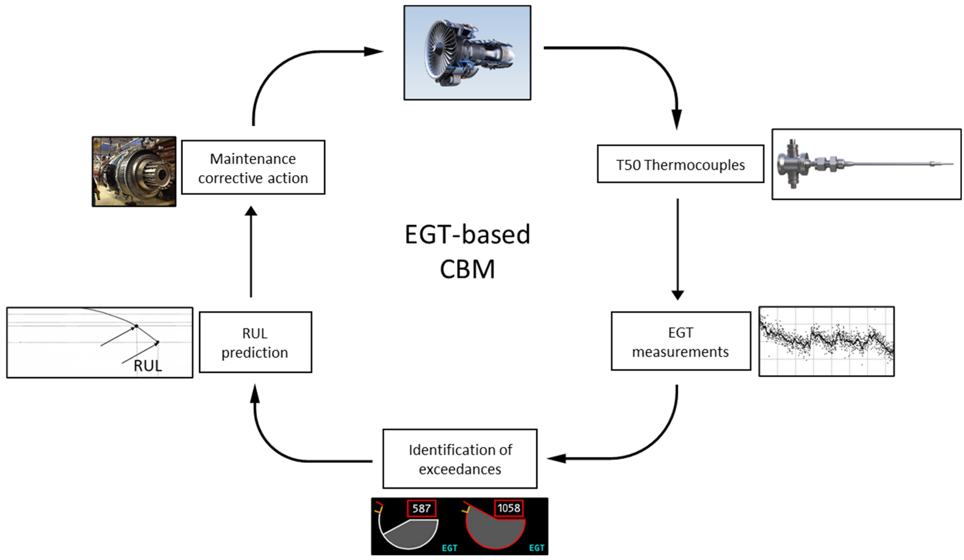
The temperature of the exhaust gases of an engine, known as the exhaust gas temperature (EGT), has evolved to become the standard industrial indicator of the health of an aircraft engine. This is because it can capture the cumulative effect of deterioration in the isentropic efficiency of gas path components [13]. This paper deals with this central role of the EGT in engine maintenance actions. Given the significant operational value of the EGT as an engine health metric, the capability of predicting the EGT is considered an important step towards improvements in decision support for engine operators. In general, the EGT should always be kept under predetermined limits to ensure optimal and safe operation of an engine. With increasing deterioration of the physical condition of an engine, the mean EGT also increases with time up to a point where these limits can be exceeded. Operational procedures state that after certain exceedance instances, corrective actions must take place, with removal from the aircraft and overhaul being the most significant and impactful ones. However, trust in the measurement of the EGT and predictability in the evolution of the EGT are two important areas of research. They can anticipate possible corrective actions while minimising operational disruptions that result in major financial and customer experience repercussions. Schematically, Figure 2 shows the process that is investigated. Starting from the engine performance and the thermocouples installed annularly downstream of the low-pressure turbine (LPT), an indicated EGT is provided. Assuming an accurate EGT measurement (or prediction, as suggested here), possible exceedances can be identified or predicted. Based on the appearance of exceedances, the remaining time on-wing can be identified, and possible corrective actions, such as engine removal, can be decided.

The present study is the first, to the best of the authors’ knowledge, that deals with the prediction of the EGT using the machine learning method of the generalised additive model. The research results prove that the EGT measurement can be replaced by a data-driven model with a highly accurate outcome when using several input features that resemble the types of physical sensors installed in the aero gas turbines currently in operation. This study can also be considered a step towards predictability not only in real time but also for the future evolution of the EGT and other engine parameters, such as in cases of sensor faults, loss of calibration, or non-identifiable EGT exceedances due to sampling or averaging errors. Another significant area of interest is the trustworthiness of data-driven models for safety-critical applications. In CBM and PdM, data play an integral role in the quality of the results, so different data concepts can influence an engine EGT prediction. More specifically, the notions of completeness, curation, representativeness, sufficiency, and traceability, as well as sensor and synthetic data, must always be considered for a complete coverage of the operational design domain (ODD) while avoiding undesirable or unexpected bias [14].

2. N-CMAPSS Database and Generalised Additive Model

2.1. N-CMAPSS

2.1.1. Dataset Composition

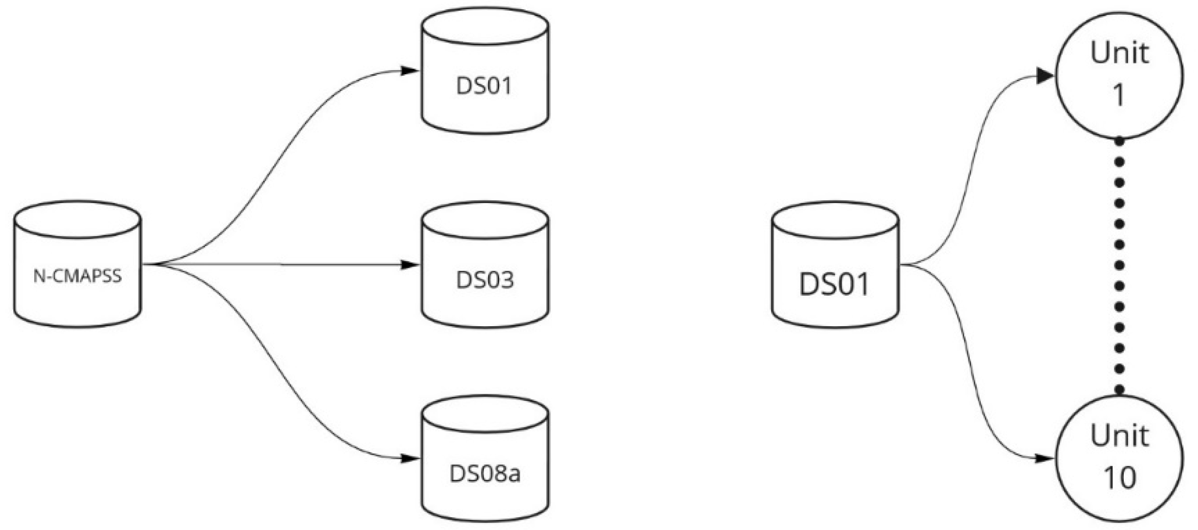
The N-CMAPSS database, developed with the use of the MATLAB’s Simulink environment [15] at NASA’s Glenn Research Center, is a public domain tool for the simulation of realistic large commercial turbofan engine data [16]. It consists of eight different datasets, each one containing run-to-failure flight data for 9–54 different engine units (Figure 3). The simulated flights include seven operational flight phases that transition linearly between each other in order to allow the engine to experience a transient phase towards each subsequent flight condition. Schematically, there is a typical ascent from sea level to a flight level of 35,000 ft and a descent back to sea level. The simulated faults are introduced at a given time and remain present throughout the remaining flights, adding to the pre-existing deterioration of the engine.

The data use a sampling rate of 1 Hz, which is a typical value for modern aero engine data recording systems [17]. The data contain 30 engine and flight parameters, not all of which are used in this present work, as explained in Section 2.1.2. Every flight in the data set contains 7 unique flight phases for a total flight time of approximately 90 min.

Table 1. N-CMAPSS database specifics and deterioration modes.

Name	# Units	Failure Modes	Fan		Low Pressure Compressor (LPC)		High Pressure Compressor (HPC)		High Pressure Turbine (HPT)		Low Pressure Turbine (LPT)		Size
			Efficiency	Mass Flow	Efficiency	Mass Flow	Efficiency	Mass Flow	Efficiency	Mass Flow	Efficiency	Mass Flow
DS01	10	1							√				7.6 M
DS02	9	2							√		√	√	6.5 M
DS03	15	1							√		√	√	9.8 M
DS04	10	1	√	√									10.0 M
DS05	10	1					√	√					6.9 M
DS06	10	1			√	√	√	√					6.8 M
DS07	10	1									√	√	7.2 M
DS08a	54	1	√	√	√	√	√	√	√	√	√	√	35.6 M

provides an overview of the composition of the datasets used, where the present characteristics are marked. The size of the different datasets is a function of the number of units monitored and of the total flight time recorded for each one of them.

The data points are available for every second of a complete flight cycle for several cycles until the end of an engine’s life. This implies that there are significant variations in the parameters measured during a cycle that are not related to deterioration but to the respective operating conditions (e.g., throttle resolver angle (TRA), Mach number, and flight altitude (FA)). In addition, compared with previously published NASA datasets, the degradation is modelled with greater fidelity; it is no longer considered linear [16]. The available features are classified into four categories:

• Flight operational parameters;
• Engine performance parameters, similar to physical engines;
• Virtual measurements, which include engine station characteristics that are not normally available or require special sensors or models to be measured and determined;
• Health parameters.

This study focuses on the engine performance parameters available in this database and summarised in

Table 2. N-CMAPSS engine performance parameters.

Symbol	Description	Units
Wf	Fuel Flow	pps
Nf	Physical fan speed	rpm
Nc	Physical core speed	rpm
T24	Total Temperature at LPC outlet	°R
T30	Total Temperature at HPC outlet	°R
T48	Total Temperature at HPT outlet	°R
T50	Total Temperature at LPT outlet	°R
P15	Total pressure in bypass duct	psia
P20	Total pressure at fan outlet	psia
P21	Total pressure at LPC inlet	psia
P24	Total pressure at LPC outlet	psia
Ps30	Static pressure at HPC outlet	psia
P40	Total pressure at combustor outlet	psia
P50	Total pressure at LPT outlet	psia

. The prediction model will be employed on the N-CMAPSS sub-datasets DS01, DS03, and DS08a. These three sub-datasets were chosen in order to explore the accuracy of the model under different deterioration scenarios. The DS01 dataset is the simplest with a single component deterioration mode (HPT efficiency), the DS03 dataset has three component deterioration modes (HPT efficiency, LPT efficiency, and mass flow capacity) and DS08a, where the last dataset simulates deterioration in all gas path components in terms of both efficiency and mass flow capacity, as illustrated in Table 1.

2.1.2. Feature Selection

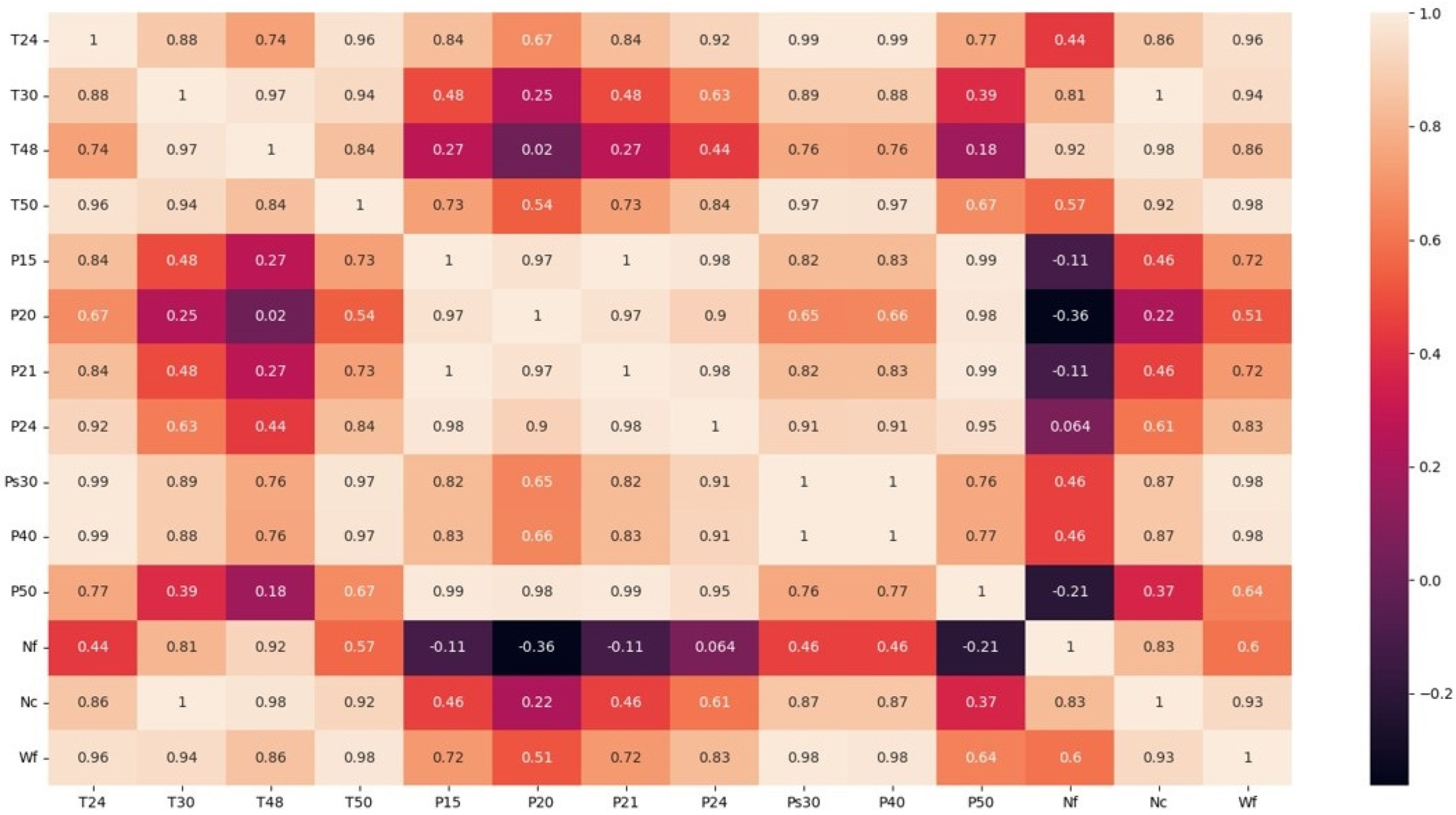
The main objective of this study is to predict the continuous value of the EGT with the use of the GAM, a machine learning method, using a set of features that represent as realistically as possible the parameters recorded in physical aero units. As a first step, a correlation matrix is put together that reveals the correlation between all the different available engine performance parameters based on the Pearson correlation method [18]. This coefficient varies between −1 and +1, with +1 indicating a perfect positive relationship between X and Y and −1 indicating a perfect negative relationship.

Out of the 14 parameters available, a selection of 6 is made for the prediction of the EGT. These six parameters represent in a realistic way the sensors installed in many popular aero engines, which are the following: T24, T30, P24, Ps30, Nc, and Wf. Based on the correlation matrix in Figure 4, we see a high degree of correlation between the above six parameters and the target parameter of T50, which represents the EGT, as station 50 is the exit of the last turbine in a turbofan engine.

2.2. Generalised Additive Model (GAM)

2.2.1. Applications of the GAM and the State of the Art

The main objective of this study is to have a prediction model of the EGT that will allow us to discuss its trustworthiness. The importance of using explainable artificial intelligence (XAI) models in predictive maintenance is explained in [19]. Furthermore, in [20], the GAM was mentioned as a complexity-related machine learning method. Concretely, the interpretability of a model is often (but not always) related to its complexity. Thus, one way of having an interpretable model is to develop it to be interpretable by construction, which is a valid statement for GAM models. The main question that needs to be answered in relation with the model is the following: How does the model arrive at a specific prediction? Lou et al. [21] called this intelligibility and stated that the GAM fulfils it, rendering the method suitable for understanding the influence of every feature in the final prediction result. Further information about the interpretability of machine learning models is available in [22] as well as in [23].

To the authors’ knowledge, there are no works using the GAM in predictive maintenance and few in aviation in general. Below are three different aviation-related works using the GAM. First, the authors of [24] compared a GAM with linear regression in order to predict aviation weather parameters. In [25], GAMs were explored because of their ability to provide information on the significance of each individual feature. The data employed in this study are flight test data, with the objective of having a physical interpretation of an aerodynamic model. Lastly, a comparative study [26] explored several machine learning models, including the GAM, in order to identify the normal behaviour of operational parameters including the power generated and blade path temperature spread.

2.2.2. Implementation of the GAM in EGT Prediction

The GAM is a machine learning method that employs linear models. Unlike other linear models, it does not simply sum up the weighted features, but it sums up the arbitrary functions for each feature. These functions allow nonlinear relationships and are called splines. This type of model therefore allows a great deal of flexibility and a greater possibility of explanation than other methods. With the GAM (and other similar ML methods) the influence of each feature on the prediction can be isolated, providing the maintenance engineers with valuable information so they can support their technical decisions and build trust in the model. The general GAM expression can be defined as follows:

$$g(E\left(Y|X\right)=s_0+{{\displaystyle \sum }}_{j=1}^p{s}_j\left(Xj\right)$$

(1)

where g is a link function, Y is the variable to be predicted, and E(Y|X) is the expected value of the predictor variables X_j. The s_j functions are non-parametric smooth functions in the sense that they are totally determined by the values of the predictor’s X_j variables. The problem at hand is a linear GAM employing a predetermined predictor, eventually being expressed as follows:

E(T50|predictor) = s₀ + s₁(T24) + s₂(T30) + s₃(P24) + s₄(Ps30) + s₅(Nc) + s₆(Wf)

(2)

The most significant hyperparameters of the GAM are denoted as λ_i and are associated with each smooth function s_i. The λ_i values are smoothing parameters that control how much of a penalty one wants to impose on the model. A higher value of λ_i results in a smoother curve. A study will be carried out to see the influence of λ_i on the quality of the prediction.

The GAM is further explained in [27], which discusses the theoretical foundations of the model. In addition, [28] also provides a more detailed overview of the implementation of GAMs and provides more information on the adaptability of the method.

3. Model Development

3.1. Data Preparation

The data used include the features selected in Section 2.1.2 for every engine unit during their total lifetimes with a sampling rate of 1 Hz. The data were divided into a training set and a test set at proportions of 70% and 30%, respectively. Standardisation was tested, but the results were not improved significantly, and thus no standardisation was chosen for the final model.

3.2. Hyperparameter Selection

This task aims to find the best lambda parameters for each spline associated to a feature of the predictor. To accomplish this, 100 λ_i values between 10⁻³ and 10³ were randomly generated, and then cross-validation was performed to determine which combinations gave the best model result. As the choice of λ_i to be tested was made randomly, the test was carried out several times to see if the results remained the same. A strucured grid search was rejected, as there was no indicative range of known hyperparameter values expected to perform well, making the process time-consuming. Instead, random selection was faster for this parameter space.

The choices for the hyperparameters are summarised in

Table 3. Hyperparameter values.

Hyperparameter	Value
n_splines	10
λi	0.6
Percentage training set	70%
Percentage test set	30%

. The parameter n_splines represents the number of basis functions used for each smooth function s_i. It should be noted that the higher the number of basis functions, the more flexible the model was, and it was the smooth parameters λ_i that aimed to regularise this. However, the more basis functions there were, the more complex the fitting of the model was. It was therefore necessary to find a balance between the two directions. The present model was developed in Python with the use of the PyGAM library [29]. In the library used, the number of basis functions was initially set to 20, but during the study, it was observed that a value of 10 was sufficient.

3.3. Model Summary

This section summarises the method used for data preparation and model training and evaluation. Figure 5 summarises the data preparation, the features selected, and the split of the data, while Figure 6 illustrates the unique trained model for each training set, which means that each unit would have an associated GAM for prediction. Lastly, Figure 7 describes the performance evaluation of each model. More specifically, the trained GAM was given the values of the test or training predictors, depending on whether the model was evaluated on the test or training data. The model thus predicted the values of the EGT, and with these predicted data and the real values, some relevant metrics were used to assess the performance of the model.

3.4. Performance Metrics

In order to assess the performance of the model, the root mean square error (RMSE) is calculated and presented in Equation (3):

$$RMSE=\sqrt{\frac{1}{N}{{\displaystyle \sum }}_{j=1}^N\left(T50j-\widehat{T50j}\right)²}$$

(3)

where N is the size of the dataset, T50j are the real values of the EGT, and $\widehat{T50j}$ represents the predicted values of the EGT. In addition, the R² score is summarised in Equation (4):

$$R^2=1-\frac{{{\displaystyle \sum }}_{j=1}^N\left(T50j-\widehat{T50j}\right)²}{{{\displaystyle \sum }}_{j=1}^N\left(T50j-\overline{T50j}\right)²}$$

(4)

The same variables are used as those above with the addition of $\overline{T50}$, which represents the arithmetic mean of the real EGT values.

4. EGT Prediction Results

For each dataset, we will summarise the results obtained for the prediction of the EGT with the two previously chosen metrics.

4.1. DS01

This dataset is the simplest one, as it introduces only deterioration in the efficiency of the HPT.

Table 4. RMSE and R² per unit for DS01.

Unit	RMSE Training	RMSE Test	R2 Training	R2 Test
1	0.5769	1.714	0.9999	0.9991
2	1.005	2.636	0.9997	0.9981
3	0.8482	1.463	0.9998	0.9994
4	0.6068	1.89	0.9998	0.9989
5	0.7985	2.067	0.9998	0.9987
6	0.8289	1.992	0.9998	0.9989
7	0.6169	2.214	0.9998	0.9985
8	0.8397	1.728	0.9998	0.9992
9	0.5793	2.675	0.9998	0.998
10	0.9154	2.149	0.9997	0.9988

shows the RMSE and R² values for the training and test set for each unit.

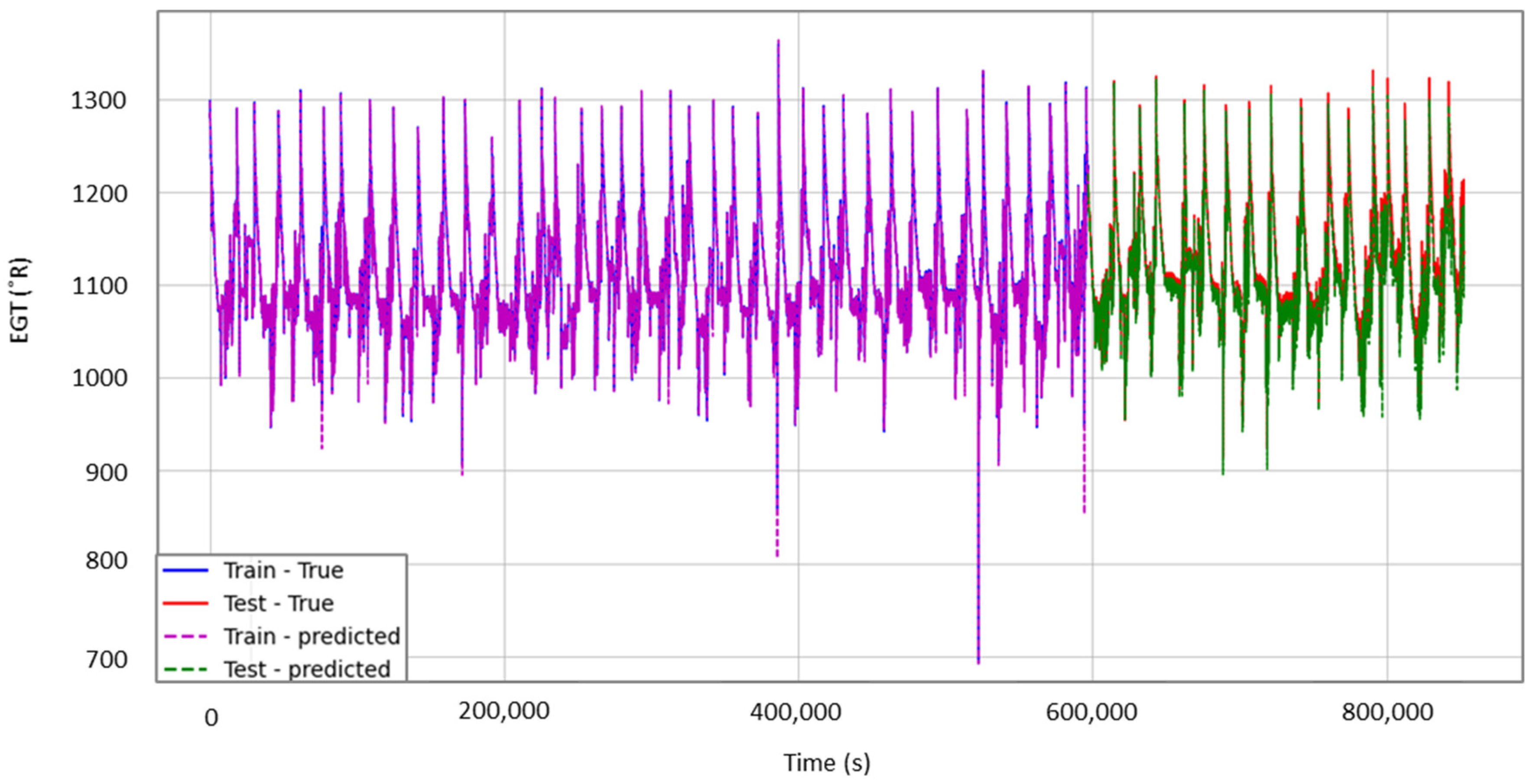
Based on the provided results, it can be concluded that the model worked well for the test set, with R² consistently being over 0.998 and the RMSE being between 3 °R and 1 °R, and an EGT equalling from 1.7 °C to 0.6 °C, a small range of EGT values. Figure 8 illustrates the evolution of T50 (EGT) for unit 9 as a function of time in seconds, highlighting the high result quality implied by the RMSE and R² values. The predicted and actual values of T50 were superimposed. The purple colour represents the predicted value, and the blue colour represents the real values of the EGT, with both corresponding to the training set. Similarly, the green colour represents the predicted EGT values, and red represents the real values for the test set. The overlap between the predicted and real values is indicative of the accuracy of the prediction, which followed the evolution of the EGT for every second, while taking into account the deterioration in the efficiency of the HPT. As this dataset does not represent an engine in commercial operation, a redline EGT is not applicable, and any possible exceedances cannot be quantified before such a criterion has been set. The variation in the EGT is indicative of the operating conditions for the seven different flight phases for every flight cycle.

4.2. DS03

This dataset is slightly more complex, with the introduction of efficiency deterioration for the HPT and both efficiency and mass flow capacity deterioration for the LPT. Given the more complex degradation pattern, the results were expected to be less accurate than the previous ones. The results are summarised in the same way as before in

Table 5. RMSE and R² per unit for DS03.

Unit	RMSE Training	RMSE Test	R2 Training	R2 Test
1	0.567	0.9842	0.9999	0.9997
2	0.8572	1.676	0.9998	0.9993
3	0.9011	1.935	0.9997	0.999
4	0.7339	1.446	0.9998	0.9994
5	0.6137	1.143	0.9998	0.9996
6	0.9642	1.988	0.9997	0.9988
7	0.8084	2.057	0.9998	0.9989
8	1.076	2.873	0.9996	0.9977
9	0.6292	2.088	0.9998	0.9987
10	1.115	4.532	0.9996	0.9937
11	1.053	1.848	0.9996	0.999
12	0.614	1.298	0.9998	0.9995
13	1.145	3.893	0.9996	0.9961
14	0.6284	1.551	0.9998	0.9992
15	0.9011	1.565	0.9997	0.9982

.

As expected, the results were marginally worse but still very accurate. For the test set, the maximum value for the RMSE was 4.5 °R with an EGT equal to 2.5 °C, which in terms of EGT error is satisfactory. As for R², the lowest value was 0.993, which is still an accurate outcome. Figure 9 shows again the evolution of T50 (EGT) versus the time in seconds for unit 10 of this dataset. The colour schemes are used the same way as explained previously. Similarly, as this dataset does not represent an engine in commercial operation, a redline EGT is not applicable, and any possible exceedances cannot be quantified before such a criterion has been set. The variation in the EGT is indicative of the operating conditions for the seven different flight phases for every flight cycle.

4.3. DS08a

This last dataset is the most complex, as every gas path component deteriorates in both efficiency and mass flow capacity. The expectation was that the prediction would be the least accurate among the three datasets presented.

Table 6. RMSE and R² per unit for DS08a.

Unit	RMSE Training	RMSE Test	R2 Training	R2 Test
1	0.6618	4.372	0.9998	0.9944
2	0.9962	1.545	0.9997	0.9993
3	0.5946	3.079	0.9998	0.9969
4	0.9608	7.239	0.9997	0.9865
5	0.9292	3.906	0.9997	0.9959
6	0.9435	1.973	0.9997	0.9989
7	0.7984	4.632	0.9998	0.9951
8	0.8011	1.472	0.9998	0.9994
9	0.667	1.751	0.9998	0.9992
10	0.6965	5.281	0.9998	0.993
11	0.878	1.098	0.9998	0.9996
12	0.9649	5.705	0.9997	0.9915
13	1.529	12.78	0.9993	0.9536
14	1.045	1.246	0.9997	0.9995
15	0.5901	2.227	0.9999	0.9986

summarises the results in the same format as DS01 and DS03 and with the same considerations regarding the EGT redline and range of values.

The test results were very close to those of dataset DS03. There were some units that were less accurate (e.g., unit 13), with an RMSE of 12.78 °R, which translated into approximately 7 °C, an acceptable value for marginal cases. The corresponding R² in this case was 0.95. However, the majority of the predictions were accurate, with an RMSE varying between 5 and 1 and R² varying between 0.998 and 0.999. Figure 10 illustrates again the evolution of T50 (EGT) as a function of time in seconds for unit 13, which was the worst performing unit.

5. Trustworthiness Considerations: Data Concepts

A fundamental need for every ML-based system such as the GAM is the collection of data to be used for training, testing, and sometimes validation purposes. In this context, several main data concepts were identified to describe aspects that needed to be considered for the development of a data management process for safety-critical applications in aviation. The prediction of the EGT, as examined in this work, is a safety-critical process indeed, since possible EGT exceedances might indicate poor engine health. The N-CMAPSS data used in this work were from a synthetic dataset, which is a special case in terms of data characteristics. However, the concepts described in this section apply to every database dealing with the problematics of data-driven CBM, and in this context, their applicability to engine-related problems will be discussed.

In general, the data concepts in this section feed the data management processes of source identification, collection, preparation, and allocation of data, essentially facilitating a common understanding of the notions of data among different parties. Moreover, some data concepts aim at the identification of potential concerns and suggest related mitigation actions, such as how to ensure that the data provide complete coverage of the operational design domain while avoiding undesirable bias. Lastly, the data concept descriptions provide some concrete guidelines.

The data concepts that were identified to be explored included bias, completeness, curation, representativeness, sensors, sufficiency, synthetic data, and traceability:

Bias. The common definition of data bias is that the available data are not representative of the population being studied. Bias in machine learning, such as GAMs, is an anomaly in the output of the algorithm [30]. These could be due to prejudices in the training data. In the context of the problem of EGT prediction, bias is introduced by collecting data from a limited set of sources, preventing representativeness of the data. This can be a major issue indeed, since there are practically unlimited combinations of ambient and operating conditions for aircraft which need to be represented in a generic dataset. The same applies to possible wrong implementation of data sampling, cleaning, or generalisation. Eventually, a successful EGT prediction under any conditions requires the premise of bias elimination from the training dataset.

Completeness. Data completeness refers to the coverage of every possible operating condition within the training dataset (i.e., how an engine operates in different kinds of environments, ambient conditions, types of air contamination, etc.) [31]. If the data are complete, then the model will work well for the functions that it is designed to perform and will interpolate well (generalisation capability) in the intended ODD. However, if the data are not complete, then the model will only work in operating regions represented by the data and may not work in other operating regimes. In the present case of EGT prediction, incomplete data mean that any predictions might be inaccurate in the case of operating regions that were not included in the original training data.

Curation. Data curation is the organisation and integration of data collected from various sources. It involves annotation, publication, and presentation of the data such that the values of the data are maintained over time, and the data remain available for reuse and preservation [32]. Properly curated data imply robust models and reproduceable results. In the context of the prediction of the EGT, data originating from different sources should be curated with standardised processes. Version control, source tagging, standardised preprocessing and strong data governance policies in general lead to proper curation and mitigate possible unwanted effects, such as inaccurate models, the inability to replicate results, and the inability to explain poor performance in EGT prediction, which might compromise safety in extreme cases.

Representativeness. Data representativeness should not be confused with data completeness. Completeness refers to coverage, whereas representativeness refers to the correct distribution of data points. For example, an on-wing engine dataset can be complete but not representative when the distribution of data points is uneven in relation with the frequency of encountering specific operating conditions, such the number of take-offs from long vs. short runways could be mentioned and the degree of derating that each runway implies, which also affects the EGT value. An uneven distribution in data might introduce bias towards the assessment of nominal operations from a specific airfield.

Sensors. Sensors are used in all systems and subsystems of aircraft to measure the different physical parameters of their operation and generate data out of them. Applications include system control, conventional diagnostics, and data-driven diagnostics that contribute to CBM. Sensors, as physical devices, can fail and generate erroneous or no data at all. Sensor noise is also a consideration, so appropriate mitigation actions must be in place. These include redundancies by design and the development of fault identification systems. Moreover, it is important to develop methods able to detect noise, boundary exceedances, and in-range anomalies. In the case of EGT prediction by using other on-wing types of data, the assurance of proper sensor functioning is paramount.

Sufficiency. Data sufficiency refers to whether the size of the data is adequate to achieve and then verify the level of performance expected for the intended function over the operational design domain. In general, a lack of data is a well-known issue in machine learning applications, especially in cases where faults and failures need to be predicted. Aviation is a very safe industry, so failures are scarce, making data sufficiency a challenging task. There is no universal definition for the amount of data needed for specific applications, but this depends on the number of characteristics for the intended prediction, the type of algorithm, and the operational domain itself. Regarding the EGT prediction, sufficiency is ensured when there are enough data points to cover all the intended operating points the operator expects to be able to predict.

Synthetic Data. The term synthetic data refers to any production data applicable to a given situation that are not obtained by direct measurement. Synthetic data are useful for new systems that are still in the design phase for which no sensor data are available. They are also useful in cases where accessibility to real data is limited but a method or process needs to be tested. This is the case in the present work, where a synthetic public domain database, N-CMAPSS, was used in combination with a GAM in order to explore the prediction of the EGT in the case of sensor fault. An interesting point is that this database was used to simulate faults and generate data corresponding to those faults, since fault data are usually hard to come by in the field.

Traceability. Data traceability refers to the identification of data sources and their trustworthiness. The concept of traceability can apply to data and other items (e.g., requirements). The significance of data traceability stems from the fact that operational data should be traceable to their origin for appropriate interpretation and investigation purposes. It should also provide an audit trail for post-decision accountability. Traceability can be ensured with appropriate data tagging both in technical and operational terms. In the case of engine EGT prediction, tagging is important for identifying the parameter names and types (e.g., physical, synthetic, or normalised), timestamps, serial numbers, etc. In addition, tagging is important for the identification of operational parameters, such as the aircraft operator or route.

6. Discussion

This study is the first, to our knowledge, that deals with the prediction of the EGT using the machine learning method of the generalised additive model. The decision to develop an EGT prediction framework stems from the fact that the exhaust gas temperature has always been the main gas turbine health-monitoring metric, and most of the crucial operational decisions are being made on the basis of the measured EGT. The reason for this preference is the fact that the EGT provides a very good indication of the accumulated thermal inefficiencies of the gas path components, being essentially a metric for a wide range of deterioration modes in safety-critical parts. Being able to predict the EGT has been considered a step towards improvement in decision support for engine operators, given its significant operational weight. Despite the fact that the EGT is measured by thermocouples installed in an annular configuration right downstream of the LPT (also known as T50), the present study has proven that this measurement can be replaced by a data-driven model with a highly accurate outcome. This study can also be considered as a first step towards predictability not only in real time but also for the future evolution of the EGT. Some reasons for replacing the measurement of the EGT in the future is that ML models such as GAMs can learn from large numbers of operating data points, essentially providing results of high fidelity even in cases of sensor faults, loss of calibration, or EGT exceedances that are not properly identified due to sampling shortcomings.

An equally important point is that all the features used for the EGT prediction were selected to emulate the physical sensors that can be found in the majority of currently operational designs by the most popular aero engine manufacturers. Given the correlations identified in the presented correlation matrix, an interesting next step is to repeat the same exercise for some of these features and assess the predictive capabilities of GAMs for them. The expansion of this study could also result in a more generalised framework for the prediction of missing engine parameters, which can then be used for health monitoring or even control in the extreme case of an engine losing its capability to measure some critical parameters entirely. In other words, this study can be considered a step towards safer flight operations with the assistance of data-driven parameter prediction.

Another area that is important to discuss is the selection of data that enabled these predictions. The authors considered the use of real operational data, but they selected the well-established N-CMAPSS database for a number of reasons. First, the globally acknowledged quality of this database ensures that the results are not compromised by data quality issues, so the conclusions can be interpreted only from the perspective of the predictive capabilities of the method. Second, the deterioration modes introduced by the different employed datasets (DS01, DS03, and DS08a) mean that the predictive capabilities of the method can also be tested in controlled conditions that take into consideration the physical evolution of engine degradation. Moreover, the increasing complexity of the datasets allows for a comparison of the accuracy of the predictions based on the complexity of the simulated operating points.

A final objective of such methods is the building of trust in predictions made by ML algorithms. The transparency of the GAM as an algorithm, in combination with the accuracy of the obtained results, gives a first indication that trustworthiness can be ensured only if trusted data and a suitable algorithm are combined. This is a first step towards certifiable artificial intelligence for aeronautical applications. A very important element of this roadmap is data quality considerations, as presented in this work as well. A main point here is that data quality is not static; it depends on the desired application and outcome. For example, a dataset might be biased by definition, but if the objective of the application is to be used for the training of an algorithm that focuses only on a specific range within the operational design domain, then this might not be a problem. However, the development of such methods requires an excellent understanding of the problem and its applications so lack of bias, completeness, representativeness and traceability can be ensured to the degree that they satisfy the problem requirements.

To summarise, despite the highly encouraging results, future research could focus on the expansion of the prediction horizon. It can also include input from other databases, either synthetic or real ones. Moreover, different combinations of features can be examined in order to emulate different faults in engine parameter measurement in real conditions. Lastly, the trustworthiness considerations of the method can be expanded by detailed research of the employed real datasets, so any shortcomings are always revealed, discussed, and addressed from the perspective of AI certifiability.

References

1. Apostolidis, A.; Stamoulis, K.P. A Health Monitoring Modelling Case Study: Humidity Effects on Engine Deterioration Prediction. MATEC Web Conf. 2021, 349, 03011. [Google Scholar] [CrossRef]
2. Nguyen, D.V.; Kefalas, M.; Yang, K.; Apostolidis, A.; Olhofer, M.; Limmer, S.; Bäck, T.H. A Review: Prognostics and Health Management in Automotive and Aerospace. Int. J. Progn. Health Manag. 2019, 10, 1–35. [Google Scholar] [CrossRef]
3. Rajamani, R. Condition-Based Maintenance in Aviation: The History, The Business and The Technology, 1st ed.; SAE International: Warrendale, PA, USA, 2018. [Google Scholar]
4. Scott, M.J.; Verhagen, W.J.C.; Bieber, M.T.; Marzocca, P. A Systematic Literature Review of Predictive Maintenance for Defence Fixed-Wing Aircraft Sustainment and Operations. Sensors 2022, 22, 7070. [Google Scholar] [CrossRef] [PubMed]
5. Baptista, M.; Sankararaman, S.; de Medeiros, I.P.; Nascimento, C., Jr.; Prendinger, H.; Henriques, E.M. Forecasting fault events for predictive maintenance using data-driven techniques and ARMA modeling. Comput. Ind. Eng. 2018, 115, 41–53. [Google Scholar] [CrossRef]
6. Fentaye, A.D.; Ul-Haq Gilani, S.I.; Baheta, A.T.; Li, Y.G. Performance-based fault diagnosis of a gas turbine engine using an integrated support vector machine and artificial neural network method. Proc. Inst. Mech. Eng. Part A J. Power Energy 2019, 233, 786–802. [Google Scholar] [CrossRef] [Green Version]
7. Protopapadakis, G.; Apostolidis, A.; Kalfas, A.I. Explainable and Interpretable AI-Assisted Remaining Useful Life Estimation for Aeroengines. In Proceedings of the ASME Turbo Expo 2022, Rotterdam, The Netherlands, 13–17 June 2022. V002T05A002. [Google Scholar] [CrossRef]
8. Apostolidis, A.; Pelt, M.; Stamoulis, K.P. Aviation Data Analytics in MRO Operations: Prospects and Pitfalls. In Proceedings of the 2020 Annual Reliability and Maintainability Symposium (RAMS), San Jose, CA, USA, 25–28 January 2020. [Google Scholar] [CrossRef]
9. Stamoulis, K. Innovations in the Aviation MRO: Adaptive, Digital, and Sustainable Tools for Smarter Engineering and Maintenance, 1st ed.; Eburon Academic Publishers: Amsterdam, The Netherlands, 2022; pp. 15–16. [Google Scholar]
10. Kefalas, M.; de Santiago Rojo, J., Jr.; Apostolidis, A.; van den Herik, D.; van Stein, B.; Bäck, T. Explainable Artificial Intelligence for Exhaust Gas Temperature of Turbofan Engines. J. Aerosp. Inf. Syst. 2022, 19, 447–454. [Google Scholar] [CrossRef]
11. Fentaye, A.D.; Baheta, A.T.; Gilani, S.I.; Kyprianidis, K.G. A Review on Gas Turbine Gas-Path Diagnostics: State-of-the-Art Methods, Challenges and Opportunities. Aerospace 2019, 6, 83. [Google Scholar] [CrossRef] [Green Version]
12. Tahan, M.; Tsoutsanis, E.; Muhammad, M.; Karim, Z.A. Performance-based health monitoring, diagnostics and prognostics for condition-based maintenance of gas turbines: A review. Appl. Energy 2017, 198, 122–144. [Google Scholar] [CrossRef]
13. Von Moll, A.; Behbahani, A.R.; Fralick, G.C.; Wrbanek, J.D.; Hunter, G.W. A Review of Exhaust Gas Temperature Sensing Techniques for Modern Turbine Engine Controls. In Proceedings of the 50th AIAA/ASME/SAE/ASEE Joint Propulsion Conference 2014, Cleveland, OH, USA, 28–30 July 2014. [Google Scholar] [CrossRef]
14. EASA. Concept Paper: First Usable Guidance for Level 1 Machine Learning Applications. Available online: https://www.easa.europa.eu/en/downloads/126648/en (accessed on 10 June 2022).
15. MATLAB, version 7.10.0 (R2010a); MathWorks Inc.: Natick, MA, USA, 2010.
16. NASA, C-MAPSS Aircraft Engine Simulator Data. Available online: https://data.nasa.gov/dataset/C-MAPSS-Aircraft-Engine-Simulator-Data/xaut-bemq (accessed on 10 June 2021).
17. EASA, Flight Data Monitoring on ATR Aircraft. Available online: https://www.easa.europa.eu/sites/default/files/dfu/16T0153_ATR_FDM_2016.pdf (accessed on 14 September 2022).
18. Boslaugh, S. Statistics in a Nutshell, 2nd ed.; O’Reilly Media: Cambridge, UK, 2014. [Google Scholar]
19. Shukla, B.; Fan, I.S.; Jennions, I. Opportunities for Explainable Artificial Intelligence in Aerospace Predictive Maintenance. In Proceedings of the PHM Society European Conference, Turin, Italy, 1–3 July 2020; Volume 5, pp. 5–11. [Google Scholar] [CrossRef]
20. Adadi, A.; Berrada, M. Peeking inside the black-box: A survey on Explainable Artificial Intelligence (XAI). IEEE Access 2018, 6, 52138–52160. [Google Scholar] [CrossRef]
21. Lou, Y.; Caruana, R.; Gehrke, J. Intelligible Models for Classification and Regression. In Proceedings of the 18th ACM SIGKDD International Conference on Knowledge Discovery and Data Mining, Beijing, China, 12–16 August 2012; pp. 150–158. [Google Scholar] [CrossRef] [Green Version]
22. Carvalho, D.V.; Pereira, E.M.; Cardoso, J.S. Machine Learning Interpretability: A Survey on Methods and Metrics. Electronics 2019, 8, 832. [Google Scholar] [CrossRef] [Green Version]
23. Molnar, C. Interpretable Machine Learning. 2019. Available online: https://christophm.github.io/interpretable-ml-book/ (accessed on 22 August 2022).
24. Vislocky, R.L.; Fritsch, J.M. Generalized Additive Models versus Linear Regression in Generating Probabilistic MOS Forecasts of Aviation Weather Parameters. Weather Forecast. 1995, 10, 669–680. [Google Scholar] [CrossRef]
25. Monstein, R.; Capone, P.; Dettling, M.; Vrdoljak, M. Determination of Model Structure from Flight Test with Generalized Additive Models. J. Aircr. 2019, 56, 1367–1375. [Google Scholar] [CrossRef]
26. Goyal, V.; Xu, M.; Kapat, J.; Vesely, L. Prediction of gas turbine performance using machine learning methods. In Proceedings of the ASME Turbo Expo 2020, Virtual Conference, Online, 21–25 September 2020; Volume 6. V006T09A004. [Google Scholar] [CrossRef]
27. Hastie, T.; Tibshirani, R. Generalized Additive Models. Stat. Sci. 1986, 1, 297–310. [Google Scholar] [CrossRef]
28. Larsen, K. GAM: The Predictive Modeling Silver Bullet. 2015. Available online: https://multithreaded.stitchfix.com/assets/files/gam.pdf (accessed on 24 August 2022).
29. pyGAM. Available online: https://pygam.readthedocs.io/en/latest/ (accessed on 24 July 2022).
30. Towards Data Science: What Is Bias? Available online: https://towardsdatascience.com/what-is-ai-bias-6606a3bcb814 (accessed on 28 September 2022).
31. Smartbridge, Data Done Right: 6 Dimensions of Data Quality. Available online: https://smartbridge.com/data-done-right-6-dimensions-of-data-quality/ (accessed on 28 September 2022).
32. Stonebraker, M.; Bruckner, D.; Ilyas, I.F.; Beskales, G.; Cherniack, M.; Zdonik, S.B.; Pagan, A.; Xu, S. Data Curation at Scale: The Data Tamer System. In Proceedings of the 6th Biennial Conference on Innovative Data Systems Research (CDIR’13), Asilomar, CA, USA, 6–9 January 2013. [Google Scholar]
Figure 1. Overview and components of CBM approach (adjusted from [9]).
Aerospace 09 00722 g001
Figure 2. Conceptual EGT-based CBM process steps.
Aerospace 09 00722 g002
Figure 3. N-CMAPSS database structure.
Aerospace 09 00722 g003
Figure 4. Performance parameters correlation matrix (DS08a).
Aerospace 09 00722 g004
Figure 5. Data preprocessing.
Aerospace 09 00722 g005
Figure 6. Unique model training.
Aerospace 09 00722 g006
Figure 7. Model evaluation.
Aerospace 09 00722 g007
Figure 8. T50 (EGT) prediction for unit 9 of DS01.
Aerospace 09 00722 g008
Figure 9. T50 (EGT) prediction for unit 10 of DS03.
Aerospace 09 00722 g009
Figure 10. T50 (EGT) prediction for unit 13 of DS08a.
Aerospace 09 00722 g010