Abstract
Considering grid requirements of high Reynolds flow, wall-modeled large eddy simulation (WMLES) and detached eddy simulation (DES) have become the main methods to deal with near-wall turbulence. However, the flow separation phenomenon is a challenge. Three typical separated flows, including flow over a cylinder at = 3900 based on the cylinder diameter, flow over a wall-mounted hump at = 9.36 × 10⁵ based on the hump length, and transonic flow over an axisymmetric bump with shock-induced separation at = 2.763 × 10⁶ based on the bump length, are used to verify WMLES, shear stress transport k- DES (SST-DES), and Spalart–Allmaras DES (SA-DES) methods in OpenFOAM. The three flows are increasingly challenging, namely laminar boundary layer separation, turbulent boundary layer separation, and turbulent boundary layer separation under shock interference. The results show that WMLES, SST-DES, and SA-DES methods in OpenFOAM can easily predict the separation position and wake characteristics in the flow around the cylinder, but they rely on the grid scale and turbulent inflow to accurately simulate the latter two flows. The grid requirements of Larsson et al. () are the basis for simulating turbulent boundary layers upstream of flow separation. A finer mesh () is required to accurately predict the separation and reattachment. The WMLES method is more sensitive to grid scales than the SA-DES method and fails to obtain flow separation under a coarser grid, while SST-DES method can only describe the vortices generated by the separating shear layer, but not within the turbulent boundary layer, and overestimates the separation-reattachment zone based on the grid system in this paper.
1. Introduction
In 1963, the large eddy simulation (LES) technique was initially proposed by Smagorinsky to simulate atmospheric current [1]. LES has been applied in unsteady, multiscale, and multi-physics turbulent flows including atomization, combustion, acoustics, and atmospheric boundary layer [2,3,4,5,6]. However, turbulent boundary layers with high Reynolds numbers would incur huge computational costs for wall-resolved LES (WRLES) that almost match the direct numerical simulation (DNS) method. Choi and Moin [7] estimated the grid requirements for a turbulent flat plate flow for DNS, wall-resolved LES, and wall-modeled LES (WMLES), which are of the order of , and , respectively. Here is the length of the flat plate. Various wall-modeled approaches for the turbulence in the inner part of the boundary layer are designed to remove the need to resolve any turbulent eddies here. These wall-modeled approaches are mainly divided into hybrid Reynolds-averaged Navier–Stokes (RANS)/LES and WMLES based on wall shear stress [8,9,10].
To keep the multiscale nature in the turbulent boundary layer, these WMLES methods are more demanding on the grid requirements than RANS methods. The grid requirements are separated in LES domain and near-wall modeled domain. Larsson [9] estimated grid requirements for the LES domain in the outer boundary layer (or ) as , where is the boundary layer thickness. Menter [11] estimated a lower requirement, . The grid requirements for the inner layer (i.e., the viscous and logarithmic layers) are further adapted to the RANS method or the modeled method based on wall shear stress. Figure 1 shows turbulence structures in a channel flow at based on three grid systems, where H is the height of the channel, is the kinematic viscosity, and is the friction velocity defined from the wall stress and the density . The first grid is commonly used in the RANS method, which relaxes the requirements on the streamwise grid size and does not obtain the vortex size. The second set of grids is obtained by refining its streamwise grid size, and the large-scale vortices in the outer layer can be obtained. Finer vortex structures can be obtained by further adopting a near-wall refined cubic mesh. Therefore, due to the requirements of WMLES on the streamwise and spanwise grid size of the region of interest, including boundary layers, separation layers and wakes, the structural grid with local refinement is an effective choice to control the total grid count.
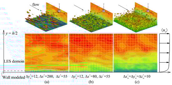
Figure 1.
Turbulence structures in a channel flow at based on three grid systems.
OpenFOAM, as a free and open-source computational fluid dynamics (CFD) software, includes several common hybrid RANS/LES methods, including Spalart–Allmaras detached eddy simulation (SA-DES) [12], Spalart–Allmaras delayed DES (SA-DDES) [13], Spalart–Allmaras Improved DDES (SA-IDDES) [14], k- SST Detached Eddy Simulation (SST-DES) [15]. OpenFOAM already has an explicit LES method with various sub-grid scales (SGS) models, including classical Smagorinsky [1], wall adapting local eddy viscosity (WALE) [16], and k-equation eddy viscosity [17] models. However, there is no effective Wall-modeled LES (WMLES) method in OpenFOAM. Recently, a wall-modeled library was developed by Mukha et al. [18] and can be combined with the SGS models in OpenFOAM to form WMLES, but it only works with incompressible flows. These techniques in OpenFOAM are being successfully applied to turbulent boundary layers and simple flows at low Reynolds numbers.
Separated flows occur in a variety of applications, such as buildings, ships, vehicles, and aircraft, from low-speed incompressible flows to supersonic compressible flows. Accurate simulation of separations is critical to their design and analysis. However, separated flows over a smooth surface present a challenge to numerical simulation methods. The flow over a circular cylinder at based on the cylindrical diameter, the flow over a wall-mounted hump and the transonic flow over an axisymmetric bump are used to test various wall-modeled approaches in OpenFOAM. The flow over a circular cylinder is a simple laminar separation and has a large amount of experimental and simulation data [19,20,21,22,23,24,25,26,27,28,29,30,31,32]. Lysenko et al. [27] applied LES methods with classical Smagorinsky and dynamic k-equation eddy viscosity SGS models in OpenFOAM to the flow over a circular cylinder at . Jiang and Cheng [32] used the WALE SGS model. D’Alessandro et al. [28] used the SA-DES method and a newly developed DES model based on the -f approach. The flow over a wall-mounted hump experiment of Greenblatt et al. [33] has been chosen as a test case for the RANS models in the NASA CFDVAL2004 Workshop [34]. The transonic flow over an axisymmetric bump experiment of Bachalo et al. [35] is a test case for the NASA Revolutionary Computational Aerosciences (RCA) challenge under the Transformational Tools and Technologies (TTT) project. The latter two flows belong to NASA Turbulence Modeling Resource (TMR) website. [36] They have fully developed a turbulent boundary layer before flow separation, and even shock/boundary layer interference occurs. This study uses SA-DES, SST-DES and WMLES in OpenFOAM to simulate these three flows to assess the capability for various separated flows. The sensitivities of these methods to grid scale and turbulent inflow are also tested.
The work is organized as follows: In Section 2, SA-DES, SST-DES and WMLES based on wall shear stress in OpenFOAM are described. In Section 3, three flows over a circular cylinder, a wall-mounted hump and an axisymmetric bump and their physics models are introduced. In Section 4, the simulation results of several WMLES methods on these three flows are compared. Conclusions are listed in Section 5.
2. Numerical Methods
This section describes the WMLES and DES methods in OpenFOAM. The WMLES method uses the flow information from the classical LES near the wall to correct the wall shear stress. The DES method introduces switch functions into the RANS equations to switch the domain between RANS and LES. Their implementations on OpenFOAM framework are shown in Figure 2.
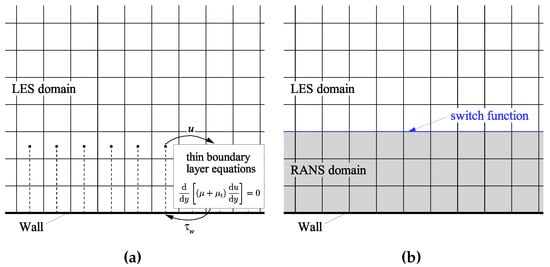
Figure 2.
Implementation of (a) WMLES and (b) DES method on OpenFOAM framework.
2.1. WMLES
In the WMLES method, the values of quantities such as pressure, density, and velocity are sampled from a specified cell center in the LES domain, located at a distance from the wall, to calculate the wall shear stress at the given surface using the wall model. Therefore, it is divided into two parts, the LES method and the wall model.
2.1.1. Governing Equations for LES
The governing equations for LES are obtained by spatial filtering of the incompressible Navier–Stokes (N-S) equations [4,5]
where t is the time, are Cartesian coordinates, is the velocity component in the direction , p and are the kinematic pressure (i.e., pressure divided by fluid density) and kinematic viscosity, respectively. The superscript denotes the resolved-scale quantity after spatial filtering, , and is the filter function. Compared with the classic N-S equations, a term with the SGS stress tensor () is added [1]. There are various methods to calculate it. Several implementations in OpenFOAM are summarized here.
Based on the assumption of the balance between the SGS energy production and dissipation (local equilibrium), Smagorinsky defined it as [1]
where is the SGS eddy viscosity, with . Here is determined by the wall adapting local eddy viscosity (WALE) model in OpenFOAM that is an algebraic eddy viscosity model taking into the rotation rate and is able to handle transition [16,37].
where is the traceless symmetric part of the square of the velocity gradient tensor . is the model constant.
2.1.2. Wall-Modeled Method
The wall stress in the inner boundary layer could be described with thin boundary layer equations [9,10]
where the turbulent eddy viscosity can be taken as , and is the normalized distance to the wall with the kinematic viscosity. The thin boundary layer equation is solved using physical quantities from a cell center in the LES domain near a wall and returns the wall shear stress to the wall. Mukha et al. [18] have implemented it for incompressible flow on the OpenFOAM framework in the form of ordinary differential equations. The current program needs to manually specify the grid point within the inner boundary layer. It should be noted that the information in the first cell near the wall cannot be sampled. When using the information of the first node as the input of the wall model, Mukha et al. [18] found deviations when simulating the channel flow, and Iyer and Malik [38] did not accurately predict the separation and reattachment. Therefore, the information from the third cell is sampled in this paper.
2.2. Detached Eddy Simulation (DES) Method
The SA-DES and SST-DES method add a switch function in the eddy viscosity -equation to switch the domain between RANS and LES, while the SST-DES method adds another switch function in the turbulent kinetic energy k-equation.
2.2.1. Spalart–Allmaras DES
Based on the Spalart–Allmaras RANS model, the SA-DES model modifies the diffusion term in the eddy viscosity -Equation [12].
Model constants , , , , and are the same as the Spalart–Allmaras RANS model. The two terms on the right side represent the production and destruction for the eddy viscosity and are related to the length scale . In DES model, it is defined as
where with . is the LES scale. is a constant and its default value is 0.65. Please note that near a wall, and Equation (5) degenerates to the Spalart–Allmaras RANS model.
2.2.2. k-ω SST DES
Based on the SST k- RANS model, The SST-DES model modifies the diffusion term in the turbulent kinetic energy k-Equation [15].
where k and are the turbulent kinetic energy and specific dissipation rate, respectively. The production terms ( and ) and switching functions ( and ) are the same as in the SST k- RANS model [15].
The switching function incorporates DES features into Equation (7).
where the turbulent length scale is . Please note that when , Equation (7) degenerates to the SST k- RANS model.
The incompressible solver pisoFoam using pressure implicit with splitting of operator (PISO) algorithm in OpenFOAM is used for the first two separation flows below, while the third uses the compressible solver myLusgsFoam developed by Fürst [39], which is a lower-upper symmetric Gauss–Seidel (LU-SGS) matrix-free solver. Compared to several compressible solvers in OpenFOAM, myLusgsFoam allows the use of larger time steps and captures shock waves using the HLLC flux scheme. The gradient and divergence terms all adopt the second-order schemes. The time terms adopt the second-order backward format. HLLC flux scheme. The HLLC fluxes for convective terms are considered in myLusgsFoam for the third transonic flow.
3. Physic Models
Three separation flows, including a flow over a circular cylinder at based on the diameter, a flow over a wall-mounted hump at based on the length of the hump, and a flow over an antisymmetric bump at and are simulated by the SA-DES, SST-DES and WMLES methods in OpenFOAM.
The computational domains for the three flows are a circular cylinder, a rectangle, and a wedge, respectively. Their geometric structure and computational domain are shown in Figure 3. Their flow conditions are summarized in Table 1. The computational domain and mesh structure for the cylinder case is consistent with the literature [27] that presented the WRLES of the flow field. The spatial domain is . The grid number is 1.44 million, which is one-fourth of the literature [27].
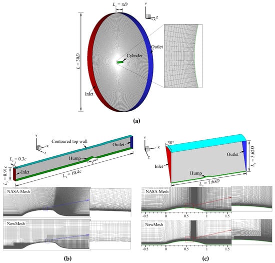
Figure 3.
Geometric structures and computational domains for (a) cylinder, (b) wall-mounted hump and (c) axisymmetric bump cases.

Table 1.
Conditions for three flows.
The length of the hump is , and its height is . The size of the computational domain corresponds to Note the geometry is two-dimensional and does not vary in the span in the simulation. Here the same spanwise dimensions as Iyer and Malik [38]. A contoured top wall is set upon the hump in the simulations based on the recommendations of the NASA CFDVAL2004 Workshop [34] to account for the effect of the side-mounted end plates in the experimental test. Two grid systems are used for the wall-mounted hump case. The first gird is from the Turbulence Modeling Resource Web of Langley Research Center, and is defined as NASA-Mesh in Figure 3. This grid has been verified to satisfy for various RANS models, but its streamwise grid size does not meet the requirements of LES. Another Cartesian grid system with prismatic boundaries is set for the wall-mounted hump case, namely NewMesh. Specific details and independent verification of NewMesh are detailed in the next section.
The transonic flow over an axisymmetric bump experiment of Bachalo et al. [35] is simulated. The length of the bump is . The domain consists of a 30° wedge with inner radius and outer radius . The bump height is . This case also uses two grid systems similar to the wall-mounted hump case.
The first two cases have similar boundary conditions. A no-slip boundary condition is imposed for the velocity at the wall. The inlet boundary condition (on the left) is a fixed-value velocity with zero-pressure gradient, while the outlet boundary condition (on the right) adopts a wave transmissive boundary with a fixed-value pressure. The boundaries on both sides of the computational domain are periodic. The third case has different settings at the inlet and outlet. There is a fixed-value velocity, total temperature, and total pressure at the inlet boundary, while there is a zero-gradient velocity, temperature and pressure at the outlet boundary. Furthermore, the incoming flow of the latter two cases is divided into laminar incoming flow and turbulent incoming flow. For turbulent incoming flow, a composite setting is used at the inlet boundary, i.e., the velocities within the turbulent boundary layer are mapped directly from a certain distance downstream, while the upper layer velocities are directly set to a fixed value, as shown in Figure 4.
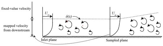
Figure 4.
Simulation method of the turbulent boundary layer at the inlet boundary.
4. Results and Discussion
4.1. Flow over a Circular Cylinder
The flow over a circular cylinder at belongs to the sub-critical regime [28]. The boundary layer is laminar, and turbulent flow only occurs after separation. There is a periodic Kármán vortex street in the wake, as shown in Figure 5. Norberg [21] measured the mean pressure distribution over a cylinder. Lourenco, Parnaudeau, Ong et al. [19,22,26] measured the flow velocity statistics in a cylindrical wake using particle image velocimetry (PIV) and hot wire anemometer (HWA). It is appropriate to use free vortices to validate numerical methods for simulating free vortices. In recent years it has been an indication of the adequacy and accuracy of LES and hybrid RANS/LES methods in OpenFOAM.
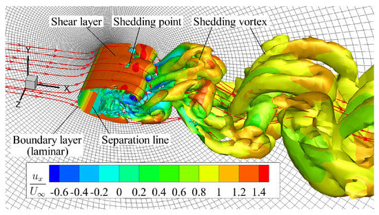
Figure 5.
Flow field structure over a circular cylinder at . (isosurface: Q-criterion).
Figure 6 shows the mean pressure coefficient distribution on the cylinder, . In addition to WMLES, SA-DES, and SST-DES, WRLES, which ignores wall-modeled approach, is also tested. In addition, WMLES also tested other SGS models in OpenFOAM to replace WALE, including classical Smagorinsky, k-equation eddy viscosity and dynamic-k-equation eddy viscosity. The results of several WMLES and DES methods show good consistency with the experimental data from Norberg [21], while that of WRLES is inaccurate.
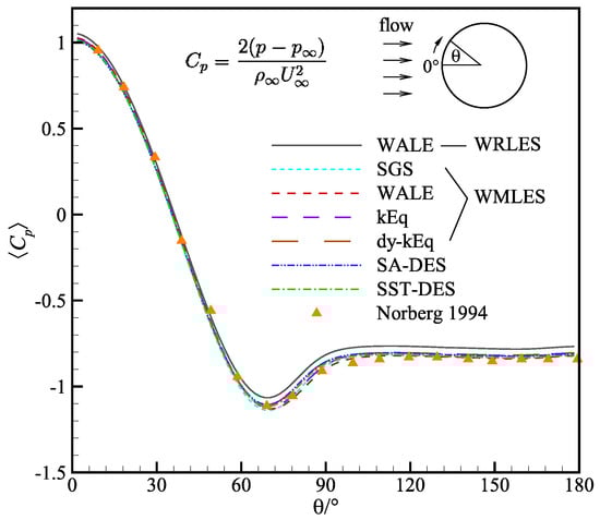
Figure 6.
Mean pressure distribution on the cylinder.
Figure 7 shows the mean velocity and resolved Reynolds stress profiles at and 1.06, 1.54, 2.02, 4, 7, 10 in the wake region. Due to the interference of the cylinder, the mean velocity profiles in Figure 7 fluctuate around , while in remote zones, they tend to converge toward freestream velocity. The mean streamwise velocity profiles are ’U’- or ’V’-shaped. The mean normal velocity profiles show an antisymmetric distribution. The mean resolved streamwise Reynolds stress profiles present a double saddle shape, and the two saddles correspond to the position of shear layers. The mean resolved normal Reynolds stress profiles present a single saddle shape. Compared with the experimental data, the mean velocity profiles of WMLES and DES methods are similar to the PIV data of Parnaudeau et al. [26] and the HWA data of Ong and Wallace [22]. There is a discrepancy with the PIV data of Lourenco and Shih [19], which may be an error from the experiment. Comparing various WMLES and DES methods, the mean velocity and resolved Reynolds stress profiles are the same.
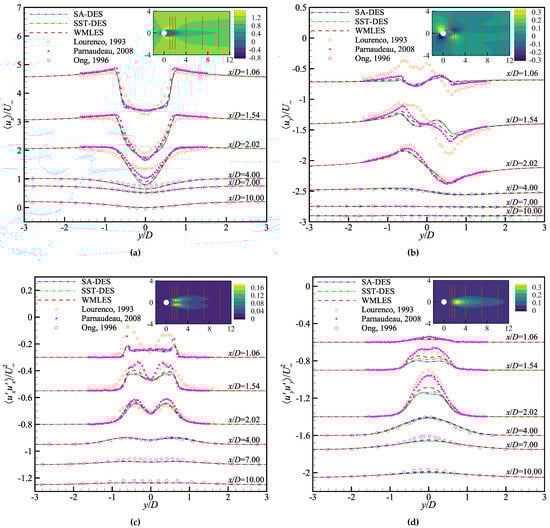
Figure 7.
Mean velocity and mean resolved Reynolds stress profiles at 1.06, 1.54, 2.02, 4.00, 7.00 and 10.00 in the wake region of cylinder: (a) Mean streamwise velocity, (b) mean normal velocity, (c) mean resolved streamwise Reynolds stress and (d) mean resolved normal Reynolds stress [19,22,26].
Figure 8 shows the power spectra of the normal velocity at in the wake. Here, 100,000 samples are recorded during the periods of . Based on the literature, the dimensionless vortex shedding frequency is , so there are about 80 vortices shedding cycles to ensure sufficient accuracy for the spectrum analysis. Figure 8 shows that the vortex shedding frequency is , which is consistent with the data of Parnaudeau et al. () [26].
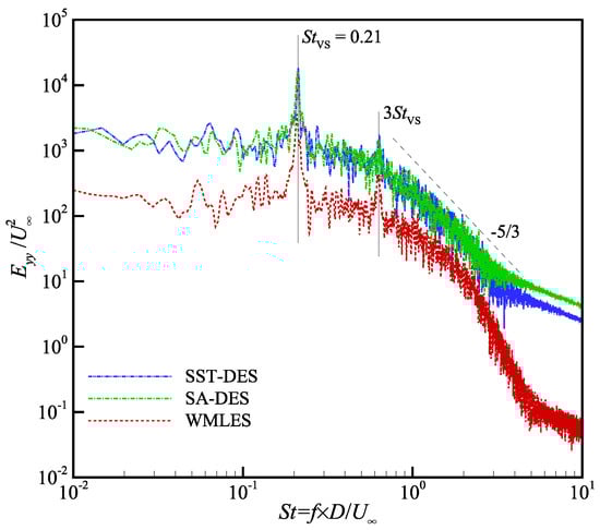
Figure 8.
Power spectra of the normal velocity at in the wake.
Table 2 summarizes some flow quantities often compared in the literature. Here denotes the mean quantity over time, and denotes the root-mean-square, is the drag coefficient, is the lift coefficient, is at stagnation point behind the cylinder, is the recirculation zone length, is the separation flow angle, and is the cell number. The integrated flow quantities obtained by each method are the same as those experimental data of Lourenco, Cardell, Norberg, Ong et al. [19,20,21,22]. In addition, Table 2 presents the simulation results of Lysenko, Tian, D’Alessandro et al. [27,28,30] using WRLES and DES methods in OpenFOAM. The grid count used in this paper is only a quarter of that of [27], but the results are as reliable as theirs. This proves that the SA-DES, SST-DES in OpenFOAM, and the WMLES developed by Mukha et al. [18] can all predict the vortex evolution caused by the laminar separated shear layer.
Table 2.
Integrated flow quantities for the flow over the cylinder at .
4.2. Flow over a Hump at
It is well known that the effect of mesh on flows at a high Reynolds number is not negligible, so mesh independence is first studied.
4.2.1. Mesh Independence of WMLES and DES
The instantaneous streamwise velocity over the wall-mounted hump in the vertical plane is shown in Figure 9a. The upstream turbulent boundary layer is accelerated on the windward side of hump, and the flow separation occurs near , forming a complex wake under the action of the strong turbulent shear layer. Figure 9b,c shows the mean streamwise velocity () and mean resolved streamwise Reynolds stress () in the vertical plane. The circulation region behind the hump is clearly visible in Figure 9b. Figure 9c indicates that there are obvious pulsations in the front side of the hump and in the wake.
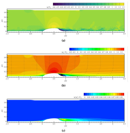
Figure 9.
(a) Instantaneous streamwise velocity, (b) mean streamwise velocity and (c) mean resolved streamwise Reynolds stress in the vertical plane.
Two grid systems mentioned in the physical model are used for simulation. The first grid system is from the NASA website and has been extensively validated for various RANS methods. Its cell number is 10.58 million. Table 3 lists the grid scales near the wall at the upstream, zenith and downstream of the hump, where is the boundary layer thickness, is the dimensionless mesh scale, and is the grid number along the boundary layer. is It can be seen that its first layer grid thickness satisfies , and there are hundreds of meshes along the boundary layer. However, the streamwise grid scale is large, especially the scale upstream is comparable to the boundary layer thickness. Considering the grid requirements of the WMLES method proposed by Larsson [9] and Menter [11], a Cartesian grid system with three prism cells near a wall is constructed using the snappyHexMesh of OpenFOAM. Its minimum streamwise grid scale is of the boundary layer thickness, and there are 21 grids along the boundary layer. The height of the first layer grid is , so the third layer grid is also located in the inner layer of the boundary layer to ensure that the wall modeling method is available. Furthermore, to prove the mesh independence of the new mesh system, two coarser and finer meshes are set, respectively, as shown in Table 4. The grid scale of the new mesh system is constant on all parts of the wall. Table 4 only gives relative quantities at , and relative quantities at other positions can be directly converted according to the boundary layer thickness given in Table 3.
Table 3.
Grid scales near the wall-mounted hump for NASA-Mesh system.
Table 4.
Grid scales near the wall-mounted hump at for NewMesh system.
The WMLES, SA-DES, and SST-DES methods are tested on these four grid systems. Figure 10 shows the mean pressure distributions on the wall-mounted hump. Compared to the WMLES result based on NASA-Mesh and coarser NewMesh, the WMLES results based on standard and finer NewMesh can reproduce the pressure step on the leeward side of the hump, which corresponds to the separation-reattachment region. Furthermore, SA-DES can predict the separation-reattachment region on the latter two grids. The prediction error of SA-DES on the first two grids is smaller than that of WMLES. However, the SST-DES results based on coarser and standard NewMesh become worse than that based on NASAmesh. This is because the SST k- method has stricter requirements on the near-wall mesh than the SA method. Therefore, the following WMLES and SA-DES results are obtained based on standard NewMesh, while SST-DES results are based on NASA-Mesh.
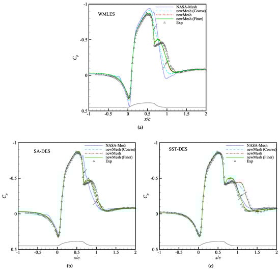
Figure 10.
Mean pressure distributions obtained by (a) WMLES, (b) SA-DES and (c) SST-DES based on different meshes.
4.2.2. Flow Predicted by DES and WMLES Methods
The flow fields predicted using SST-DES, SA-DES, and WMLES methods are compared. In addition to the turbulent inflow conditions, a laminar inflow for SA-DES and WMLES is also considered.
Figure 11 visualizes transient vortex structures using Q-criterion obtained by these methods with/without turbulent inflow. SA-DES and WMLES methods can characterize coherent structures in the incoming turbulent boundary layer, while the SST-DES method cannot. This is due to the difference in the active regions of RANS and LES obtained by SA-DES and SST-DES. Figure 12a shows the distribution of the switch function for the SA-DES method, and Figure 12b shows that of the switch function for the SST-DES method. is determined by the wall distance and grid scale, so the space far from the wall is the LES region for SA-DES. is determined by the RANS scale, grid scale and wall distance, so only the separation region is divided into the LES region for SST-DES. Therefore, the SST-DES method only models the vortex structure within the separated shear layer and the wake, while the SST-DES method identifies all the turbulent boundary layers upstream of the separation as RANS regions, as shown in Figure 11a,b. The vortex scale of the separated shear layer obtained by SST-DES is significantly larger than those of SA-DES and WMLES methods, especially those based on NASAmesh. When the incoming flow is laminar, the boundary layer is always laminar until it reaches the windward side of the hump, where the inverse pressure gradient promotes the transition. There are quasi two-dimensional vortices and -shaped vortices on the windward side of the hump in the close-up view of Figure 11d,f.
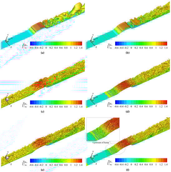
Figure 11.
Transient vortex structures visualized by iso-surface of Q-criterion colored by streamwise velocity obtained by: (a) SST-DES based on NASAMesh, (b) SST-DES based on NewMesh, (c) SA-DES with turbulent inflow, (d) SA-DES with laminar inflow, (e) WMLES with turbulent inflow and (f) WMLES with laminar inflow, where (c–f) are based on NewMesh.
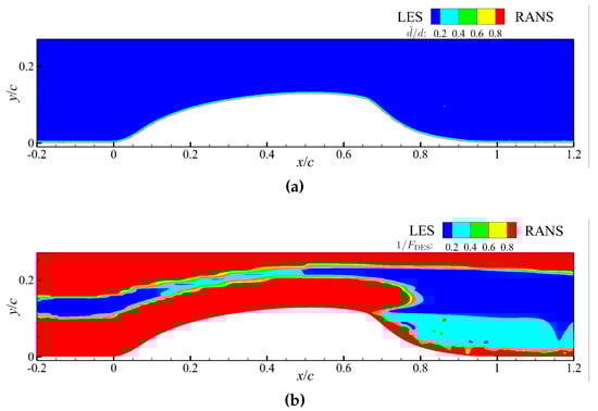
Figure 12.
Action regions of RANS and LES obtained by: (a) SA-DES and (b) SST-DES.
Figure 13 shows mean pressure distributions along the wall-mounted hump. The pressure distribution between corresponds to the separation and re-attachment circulation region behind the hump. The separation locations predicted by several numerical methods with turbulent inflow are consistent with the experimental data (), and the maximum deviation is only , as listed in Table 5. There is a certain deviation in the reattachment locations predicted by them from the experimental data (). The reattachment locations predicted by SA-DES and WMLES are shifted upstream by and , while that of SST-DES is shifted downstream by . In addition, compared to SA-DES and WMLES with turbulent inflow, they with laminar inflow predict a larger maximum pressure upstream of the hump, a smaller minimum pressure at the zenith of the hump, and a forward shift of the reattachment location.
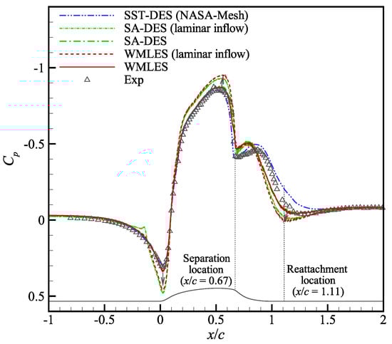
Figure 13.
Mean pressure distribution along the wall-mounted hump obtained by DES and WMLES methods with/without turbulent inflow.
Table 5.
Separation and reattachment locations predicted by several numerical methods with turbulent inflow.
Figure 14 shows the mean velocity and mean resolved Reynolds stress profiles at 0.65, 0.8, 0.9, 1.0, 1.1, 1.2, and 1.3 in the wake region. The mean velocity profiles obtained by SA-DES and WMLES is closer to the experimental data than those of SST-DES. The Reynolds mean resolved Reynolds stress profiles obtained by the first two is larger than the experimental data, while that of SST-DES is smaller. This resulted in the separation-reattachment regions predicted by SA-DES and WMLES being smaller than the experimental results.
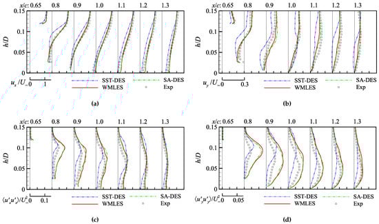
Figure 14.
Mean velocity and mean resolved Reynolds stress profiles at 0.65, 0.8, 0.9, 1.0, 1.1, 1.2 and 1.3 in the wake region of hump: (a) mean streamwise velocity, (b) mean normal velocity, (c) mean resolved streamwise Reynolds stress, and (d) mean resolved normal Reynolds stress.
The WMLES method above uses the WALE SGS model by default. Other SGS models in OpenFOAM are also tested into WMLES, including classical Smagorinsky, k-equation eddy viscosity, and dynamic-k-equation eddy viscosity. When the inflow is turbulent, their four predictions are consistent. When the inflow is laminar, the results obtained by WALE and dynamics-k-equation eddy viscosity are consistent, while the classical Smagorinsky and k-equation models cannot predict the transition upstream of the hump and obtain extra separation bubbles here.
4.3. Transonic Flow over an Axisymmetric Bump
This flow is also tested on two grid systems. Since this flow separation is induced by the adverse pressure gradient of -shock, as shown in Figure 15, the mesh is refined at the shock as well as at the boundary layer and separation zone, as shown in Figure 3c. Table 6 lists grid scales near the antisymmetric bump at for two grid systems. There is 20.74 million cells in NASA-Mesh, while NewMesh is a four-level local-refined hexahedral mesh with a total of 24.90 million cells.
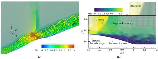
Figure 15.
Instantaneous vortex structures visualized by iso-surface of Q-crierion colored by Mach number obtained by SA-DES: (a) three-dimensional and (b) two-dimensional vertical plane.
Table 6.
Grid scales near the antisymmetric bump at for two grid systems.
Figure 16 shows the mean pressure distribution along the wall-mounted axisymmetric bump obtained by WMLES SA-DES and SST-DES methods. The result of SST RANS is also presented in Figure 16. Since this experiment has been used in the calibration of the SST model coefficients, the result of SST RANS is in agreement with the experimental data [45]. However, the reattachment position predicted by the SST-DES results based on the two grid systems is significantly shifted to the right. The pressure distribution within predicted by WMLES is linearly decreasing, indicating that it does not predict the flow separation zone. The SA-DES result is in the best agreement with the experimental data.
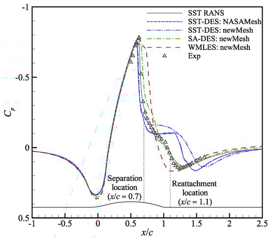
Figure 16.
Mean pressure distribution along the wall-mounted axisymmetric bump obtained by DES and WMLES methods.
Figure 17 shows the mean streamwise velocity and mean resolved Reynolds stress profiles at 0.813, 0.938, 1.0, 1.125, and 1.25 in the wake region of axisymmetric bump. The Reynolds stress in the separation zone obtained by SST-DES is almost zero, i.e., the velocity pulsation here cannot be obtained. The velocity fluctuation obtained by WMLES is much higher than the experimental data, especially near the separated shear layer at 0.813.
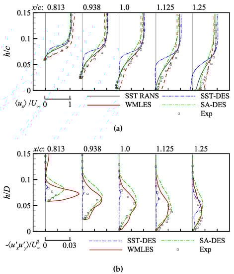
Figure 17.
(a) Mean streamwise velocity and (b) mean resolved Reynolds stress profiles at 0.813, 0.938, 1.0, 1.125 and 1.25 in the wake region of axisymmetric bump.
5. Conclusions
In this study, the WMLES, SA-DES, and SST-DES methods in OpenFOAM were tested on three separated flows, including flow over a cylinder at = 3900, separated flow over a wall-mounted hump at = 9.36 × 10⁵, and transonic flow over an axisymmetric bump with shock-induced separation at = 2.763 × 10⁶. The complexity of these three flows is gradually increasing. WMLES, SST-DES, and SA-DES methods in OpenFOAM can easily predict the separation position and wake characteristics in the flow around the cylinder, and they rely on the grid scale and turbulent inflow to accurately simulate the latter two flows.
In terms of grid independence, when the grid scales in the boundary layer meet the grid requirements proposed by Larsson et al. [9] (), it is possible to simulate the vortex structure in the turbulent boundary layer upstream of the flow separation. However, finer meshes are required to accurately predict the separation and reattachment. The second flow could be reproduced when using a three-level local-refined hexahedral mesh grid system with a near-wall grid scale of . The third flow could be reproduced when using a four-level local-refined hexahedral mesh grid system with a near-wall grid scale of . WMLES method is more sensitive to grid scales than the SA-DES method. The new grid constructed in this paper cannot meet the grid requirements of SST-DES, so its simulation results based on the structural grid system from NASA are closer to the experimental data. Table 7 summarizes grid requirements for WMLES, SA-DES, and SST-DES in OpenFOAM.
Table 7.
Grid requirements for WMLES, SA-DES and SST-DES in OpenFOAM.
In terms of vortex description, SST-DES can only simulate vortices induced by the separated shear layer, while SA-DES and WMLES can also simulate vortices in the turbulent boundary layer upstream of the flow separation. Furthermore, WMLES with WALE and dynamic-k-equation SGS models and SA-DES can simulate the transition of the laminar boundary layer in the flow over the wall-mounted hump.
Author Contributions
X.R. and H.-H.Y. designed and were responsible for running the numerical simulations, carrying out the post-processing and writing the manuscript; H.S. designed the simulation condition; Z.Y. analyzed the flow mechanism. All authors have read and agreed to the published version of the manuscript.
Funding
This research received no external funding.
Institutional Review Board Statement
Not applicable.
Informed Consent Statement
Not applicable.
Data Availability Statement
The data that support the findings of this study are available from the corresponding author upon reasonable request.
Conflicts of Interest
The authors declare no conflict of interest.
References
- Smagorinsky, J. General Circulation Experiments with the Primitive Equations: I. The Basic Experiment. Mon. Weather Rev. 1963, 91, 99–164. [Google Scholar] [CrossRef]
- Pope, S.B. Turbulent Flows; Cambridge University Press: Cambridge, MA, USA, 2000. [Google Scholar]
- Pitsch, H. Large-Eddy Simulation of Turbulent Combustion. Annu. Rev. Fluid Mech. 2006, 38, 453–482. [Google Scholar] [CrossRef]
- Sagaut, P. Large Eddy Simulation for Incompressible Flows: An Introduction; Springer Science & Business Media: Berlin/Heidelberg, Germany, 2006. [Google Scholar] [CrossRef]
- Garnier, E.; Adams, N.; Sagaut, P. Large Eddy Simulation for Compressible Flows; Scientific Computation; Springer: Dordrecht, The Netherlands, 2009. [Google Scholar] [CrossRef]
- Yang, Z. Large-Eddy Simulation: Past, Present and the Future. Chin. J. Aeronaut. 2015, 28, 11–24. [Google Scholar] [CrossRef]
- Choi, H.; Moin, P. Grid-Point Requirements for Large Eddy Simulation: Chapman’s Estimates Revisited. Phys. Fluids 2012, 24, 011702. [Google Scholar] [CrossRef]
- Piomelli, U.; Balaras, E. Wall-Layer Models for Large-Eddy Simulations. Annu. Rev. Fluid Mech. 2002, 34, 349–374. [Google Scholar] [CrossRef]
- Larsson, J.; Kawai, S.; Bodart, J.; Bermejo-Moreno, I. Large Eddy Simulation with Modeled Wall-Stress: Recent Progress and Future Directions. Mech. Eng. Rev. 2016, 3, 15-00418. [Google Scholar] [CrossRef]
- Bose, S.T.; Park, G.I. Wall-Modeled Large-Eddy Simulation for Complex Turbulent Flows. Annu. Rev. Fluid Mech. 2018, 50, 535–561. [Google Scholar] [CrossRef]
- Menter, F.R. Best Practice: Scale-Resolving Simulations in ANSYS CFD; ANSYS, Inc.: Canonsburg, PA, USA, 2012. [Google Scholar]
- Spalart, P.; Jou, W.H.; Strelets, M.; Allmaras, S. Comments on the Feasibility of LES for Wings, and on a Hybrid RANS/LES Approach. In Proceedings of the First AFOSR International Conference on DNS/LES, Ruston, LA, USA, 4–8 August 1997. [Google Scholar]
- Spalart, P.R.; Deck, S.; Shur, M.L.; Squires, K.D.; Strelets, M.K.; Travin, A. A New Version of Detached-Eddy Simulation, Resistant to Ambiguous Grid Densities. Theor. Comp. Fluid Dyn. 2006, 20, 181. [Google Scholar] [CrossRef]
- Shur, M.L.; Spalart, P.R.; Strelets, M.K.; Travin, A.K. A Hybrid RANS-LES Approach with Delayed-DES and Wall-Modelled LES Capabilities. Int. J. Heat Fluid Flow 2008, 29, 1638–1649. [Google Scholar] [CrossRef]
- Menter, F.R.; Kuntz, M.; Langtry, R. Ten Years of Industrial Experience with the SST Turbulence Model. In Proceedings of the 4th International Symposium on Turbulence, Heat and Mass Transfer, Antalya, Turkey, 12–17 October 2003; Volume 4, pp. 625–632. [Google Scholar]
- Nicoud, F.; Ducros, F. Subgrid-Scale Stress Modelling Based on the Square of the Velocity Gradient Tensor. Flow Turbul. Combust. 1999, 62, 183–200. [Google Scholar] [CrossRef]
- Yoshizawa, A. Statistical Theory for Compressible Turbulent Shear Flows, with the Application to Subgrid Modeling. Phys. Fluids 1986, 29, 2152–2164. [Google Scholar] [CrossRef]
- Mukha, T.; Rezaeiravesh, S.; Liefvendahl, M. A Library for Wall-Modelled Large-Eddy Simulation Based on OpenFOAM Technology. Comput. Phys. Commun. 2019, 239, 204–224. [Google Scholar] [CrossRef]
- Lourenco, L. Characteristics of the Plate Turbulent near Wake of a Circular Cylinder. A Particle Image Velocimetry Study. In Report No. TF62; Beaudan, P., Moin, P., Eds.; Thermosciences Division, Department of Mechanical Engineering, Stanford University: Stanford, CA, USA, 1993. [Google Scholar]
- Cardell, G.S. Flow Past a Circular Cylinder with a Permeable Wake Splitter Plate. Ph.D. Thesis, California Institute of Technology, Pasadena, CA, USA, 1993. [Google Scholar] [CrossRef]
- Norberg, C. An Experimental Investigation of the Flow around a Circular Cylinder: Influence of Aspect Ratio. J. Fluid Mech. 1994, 258, 287–316. [Google Scholar] [CrossRef]
- Ong, L.; Wallace, J. The Velocity Field of the Turbulent Very near Wake of a Circular Cylinder. Exp. Fluids 1996, 20, 441–453. [Google Scholar] [CrossRef]
- Kravchenko, A.G.; Moin, P. Numerical Studies of Flow over a Circular Cylinder at ReD=3900. Phys. Fluids 2000, 12, 403–417. [Google Scholar] [CrossRef]
- Ma, X.; Karamanos, G.S.; Karniadakis, G.E. Dynamics and Low-Dimensionality of a Turbulent near Wake. J. Fluid Mech. 2000, 410, 29–65. [Google Scholar] [CrossRef]
- Dong, S.; Karniadakis, G.E.; Ekmekci, A.; Rockwell, D. A Combined Direct Numerical Simulation-Particle Image Velocimetry Study of the Turbulent near Wake. J. Fluid Mech. 2006, 569, 185. [Google Scholar] [CrossRef]
- Parnaudeau, P.; Carlier, J.; Heitz, D.; Lamballais, E. Experimental and Numerical Studies of the Flow over a Circular Cylinder at Reynolds Number 3900. Phys. Fluids 2008, 20, 085101. [Google Scholar] [CrossRef]
- Lysenko, D.A.; Ertesvåg, I.S.; Rian, K.E. Large-Eddy Simulation of the Flow over a Circular Cylinder at Reynolds Number 3900 Using the OpenFOAM Toolbox. Flow Turbul. Combust. 2012, 89, 491–518. [Google Scholar] [CrossRef]
- D’Alessandro, V.; Montelpare, S.; Ricci, R. Detached–Eddy Simulations of the Flow over a Cylinder at Re = 3900 Using OpenFOAM. Comput. Fluids 2016, 136, 152–169. [Google Scholar] [CrossRef]
- Jiang, H.; Cheng, L. Strouhal–Reynolds Number Relationship for Flow Past a Circular Cylinder. J. Fluid Mech. 2017, 832, 170–188. [Google Scholar] [CrossRef]
- Tian, G.; Xiao, Z. New Insight on Large-Eddy Simulation of Flow Past a Circular Cylinder at Subcritical Reynolds Number 3900. AIP Adv. 2020, 10, 085321. [Google Scholar] [CrossRef]
- Jiang, H. Separation Angle for Flow Past a Circular Cylinder in the Subcritical Regime. Phys. Fluids 2020, 32, 014106. [Google Scholar] [CrossRef]
- Jiang, H.; Cheng, L. Large-Eddy Simulation of Flow Past a Circular Cylinder for Reynolds Numbers 400 to 3900. Phys. Fluids 2021, 33, 034119. [Google Scholar] [CrossRef]
- Greenblatt, D.; Paschal, K.B.; Yao, C.S.; Harris, J.; Schaeffler, N.W.; Washburn, A.E. Experimental Investigation of Separation Control Part 1: Baseline and Steady Suction. AIAA J. 2006, 44, 2820–2830. [Google Scholar] [CrossRef]
- Rumsey, C.; Gatski, T.; Sellers, W.; Vatsa, V.; Viken, S. Summary of the 2004 CFD Validation Workshop on Synthetic Jets and Turbulent Separation Control. In Proceedings of the 2nd AIAA Flow Control Conference, Portland, OR, USA, 28 June–1 July 2004; American Institute of Aeronautics and Astronautics: Reston, VA, USA, 2004; p. 2217. [Google Scholar] [CrossRef]
- Bachalo, W.D.; Johnson, D.A. Transonic, Turbulent Boundary-Layer Separation Generated on an Axisymmetric Flow Model. AIAA J. 1986, 24, 437–443. [Google Scholar] [CrossRef]
- Turbulence Modeling Resource. 2022. Available online: https://turbmodels.larc.nasa.gov/index.html (accessed on 27 October 2022).
- OpenFOAM: User Guide: Smagorinsky. Available online: https://www.openfoam.com/documentation/guides/latest/doc/guide-turbulence-les-smagorinsky.html (accessed on 27 October 2022).
- Iyer, P.S.; Malik, M. Wall–Modeled Large Eddy Simulation of Flow over a Wall–Mounted Hump. In Proceedings of the 46th AIAA Fluid Dynamics Conference, Washington, DC, USA, 13–17 June 2016. [Google Scholar] [CrossRef]
- Fürst, J. Development of a Coupled Matrix-Free LU-SGS Solver for Turbulent Compressible Flows. Comput. Fluids 2018, 172, 332–339. [Google Scholar] [CrossRef]
- Šarić, S.; Jakirlić, S.; Djugum, A.; Tropea, C. Computational Analysis of Locally Forced Flow over a Wall-Mounted Hump at High-Re Number. Int. J. Heat Fluid Flow 2006, 27, 707–720. [Google Scholar] [CrossRef]
- Wang, Y.; Vita, G.; Fraga, B.; Wang, J.; Hemida, H. Effect of the Inlet Boundary Conditions on the Flow over Complex Terrain Using Large Eddy Simulation. Designs 2021, 5, 34. [Google Scholar] [CrossRef]
- Ge, X.; De Stefano, G.; Hussaini, M.Y.; Vasilyev, O.V. Wavelet-Based Adaptive Eddy-Resolving Methods for Modeling and Simulation of Complex Wall-Bounded Compressible Turbulent Flows. Fluids 2021, 6, 331. [Google Scholar] [CrossRef]
- Park, G.I. Wall-Modeled Large-Eddy Simulation of a High Reynolds Number Separating and Reattaching Flow. AIAA J. 2017, 55, 3709–3721. [Google Scholar] [CrossRef] [PubMed]
- Uzun, A.; Malik, M. Large-Eddy Simulation of Flow over a Wall-Mounted Hump with Separation and Reattachment. AIAA J. 2017, 56, 1–16. [Google Scholar] [CrossRef]
- Uzun, A.; Malik, M.R. Wall-Resolved Large-Eddy Simulations of Transonic Shock-Induced Flow Separation. AIAA J. 2019, 57, 1955–1972. [Google Scholar] [CrossRef]


Publisher’s Note: MDPI stays neutral with regard to jurisdictional claims in published maps and institutional affiliations. |
© 2022 by the authors. Licensee MDPI, Basel, Switzerland. This article is an open access article distributed under the terms and conditions of the Creative Commons Attribution (CC BY) license (https://creativecommons.org/licenses/by/4.0/).