1. Introduction
In 1963, the large eddy simulation (LES) technique was initially proposed by Smagorinsky to simulate atmospheric current [
1]. LES has been applied in unsteady, multiscale, and multi-physics turbulent flows including atomization, combustion, acoustics, and atmospheric boundary layer [
2,
3,
4,
5,
6]. However, turbulent boundary layers with high Reynolds numbers would incur huge computational costs for wall-resolved LES (WRLES) that almost match the direct numerical simulation (DNS) method. Choi and Moin [
7] estimated the grid requirements for a turbulent flat plate flow for DNS, wall-resolved LES, and wall-modeled LES (WMLES), which are of the order of
,
and
, respectively. Here
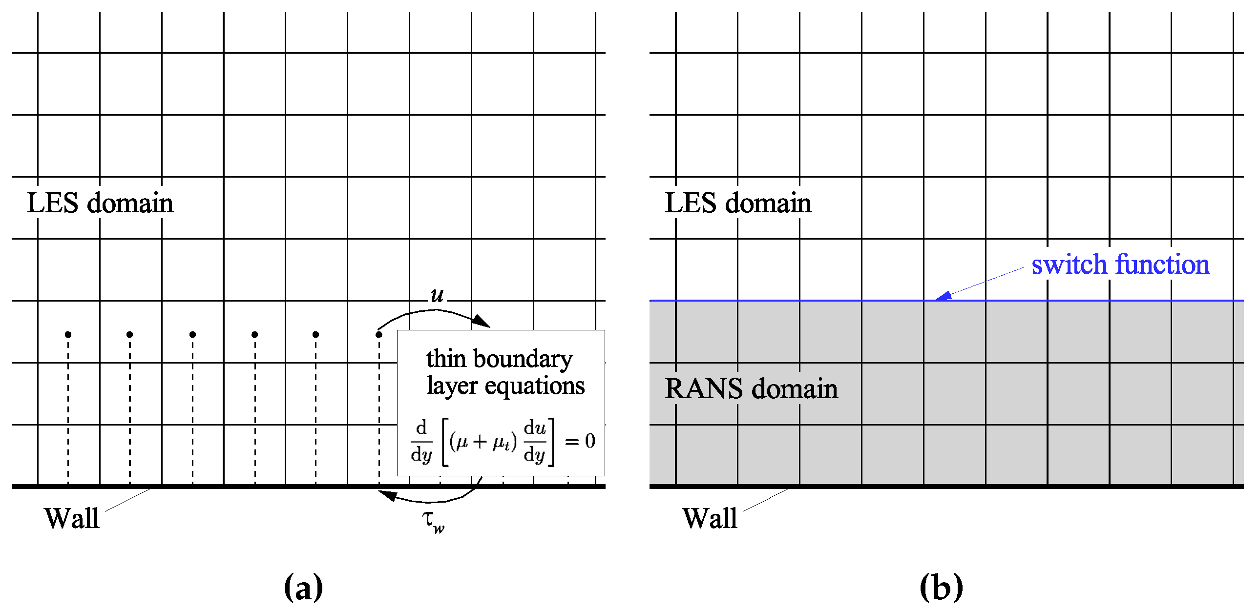
is the length of the flat plate. Various wall-modeled approaches for the turbulence in the inner part of the boundary layer are designed to remove the need to resolve any turbulent eddies here. These wall-modeled approaches are mainly divided into hybrid Reynolds-averaged Navier–Stokes (RANS)/LES and WMLES based on wall shear stress [
8,
9,
10].
To keep the multiscale nature in the turbulent boundary layer, these WMLES methods are more demanding on the grid requirements than RANS methods. The grid requirements are separated in LES domain and near-wall modeled domain. Larsson [
9] estimated grid requirements for the LES domain in the outer boundary layer (or
) as
, where
is the boundary layer thickness. Menter [
11] estimated a lower requirement,
. The grid requirements for the inner layer (i.e., the viscous and logarithmic layers) are further adapted to the RANS method or the modeled method based on wall shear stress.
Figure 1 shows turbulence structures in a channel flow at
based on three grid systems, where
H is the height of the channel,
is the kinematic viscosity, and
is the friction velocity defined from the wall stress
and the density
. The first grid is commonly used in the RANS method, which relaxes the requirements on the streamwise grid size and does not obtain the vortex size. The second set of grids is obtained by refining its streamwise grid size, and the large-scale vortices in the outer layer can be obtained. Finer vortex structures can be obtained by further adopting a near-wall refined cubic mesh. Therefore, due to the requirements of WMLES on the streamwise and spanwise grid size of the region of interest, including boundary layers, separation layers and wakes, the structural grid with local refinement is an effective choice to control the total grid count.
OpenFOAM, as a free and open-source computational fluid dynamics (CFD) software, includes several common hybrid RANS/LES methods, including Spalart–Allmaras detached eddy simulation (SA-DES) [
12], Spalart–Allmaras delayed DES (SA-DDES) [
13], Spalart–Allmaras Improved DDES (SA-IDDES) [
14],
k-
SST Detached Eddy Simulation (SST-DES) [
15]. OpenFOAM already has an explicit LES method with various sub-grid scales (SGS) models, including classical Smagorinsky [
1], wall adapting local eddy viscosity (WALE) [
16], and
k-equation eddy viscosity [
17] models. However, there is no effective Wall-modeled LES (WMLES) method in OpenFOAM. Recently, a wall-modeled library was developed by Mukha et al. [
18] and can be combined with the SGS models in OpenFOAM to form WMLES, but it only works with incompressible flows. These techniques in OpenFOAM are being successfully applied to turbulent boundary layers and simple flows at low Reynolds numbers.
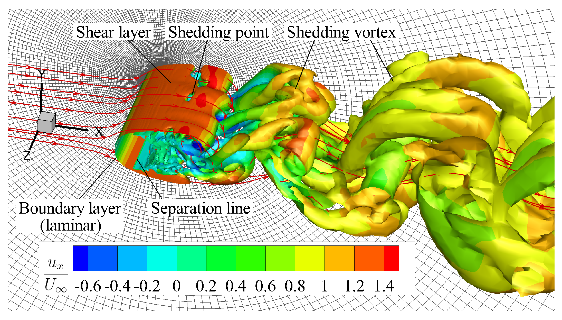
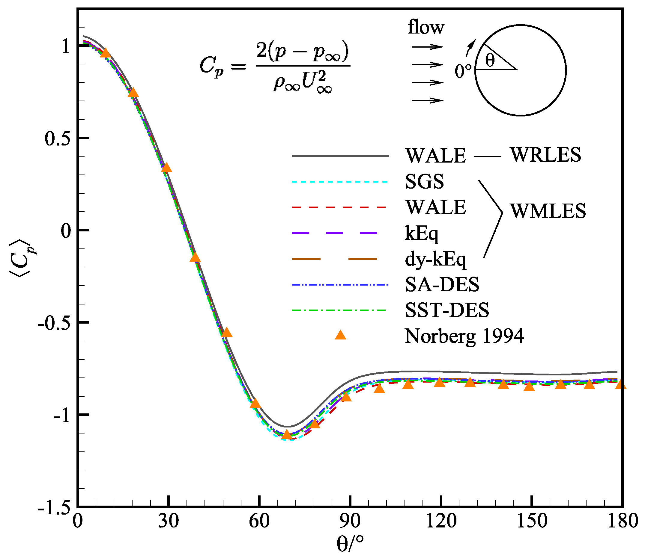
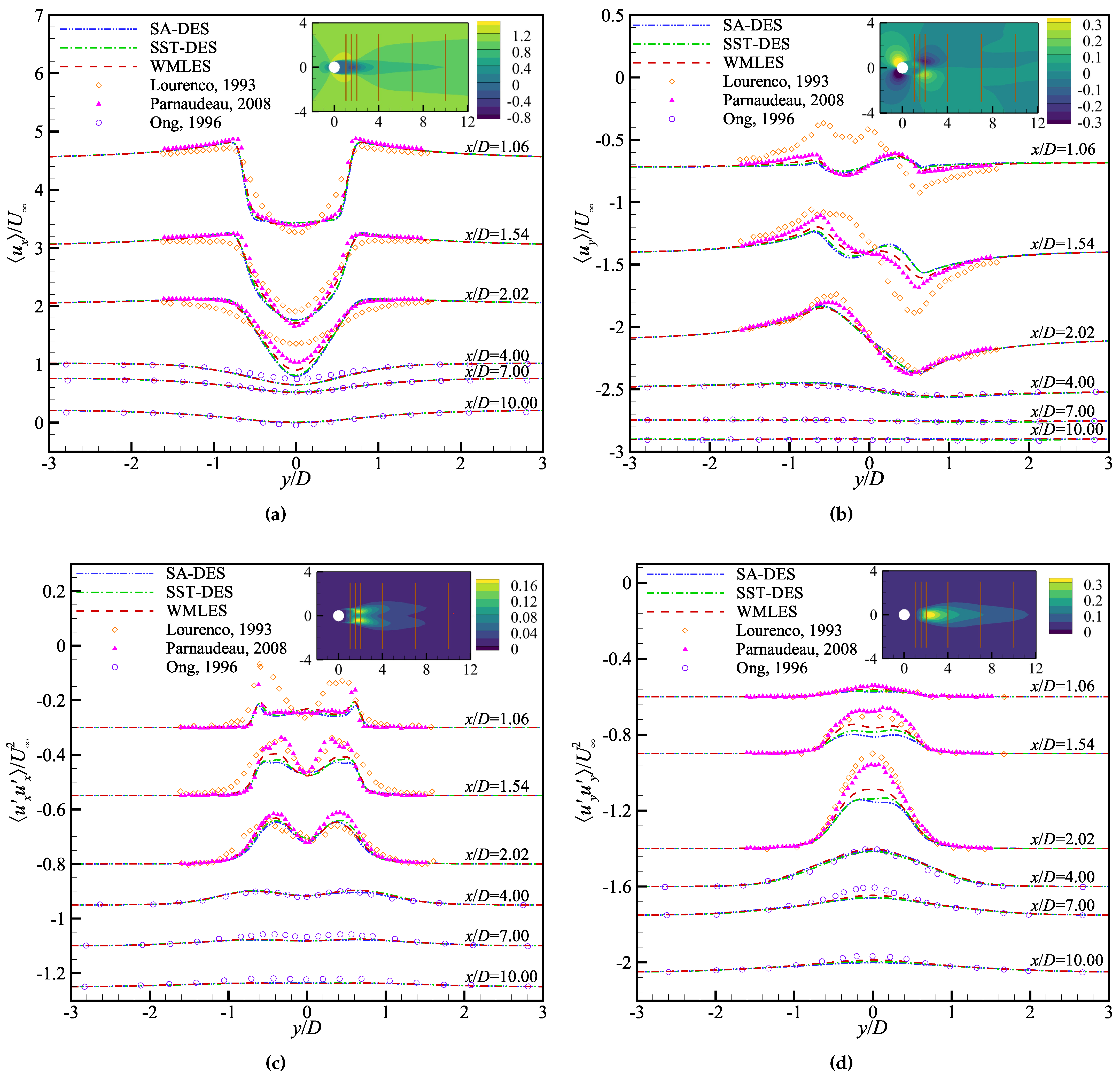
Separated flows occur in a variety of applications, such as buildings, ships, vehicles, and aircraft, from low-speed incompressible flows to supersonic compressible flows. Accurate simulation of separations is critical to their design and analysis. However, separated flows over a smooth surface present a challenge to numerical simulation methods. The flow over a circular cylinder at
based on the cylindrical diameter, the flow over a wall-mounted hump and the transonic flow over an axisymmetric bump are used to test various wall-modeled approaches in OpenFOAM. The flow over a circular cylinder is a simple laminar separation and has a large amount of experimental and simulation data [
19,
20,
21,
22,
23,
24,
25,
26,
27,
28,
29,
30,
31,
32]. Lysenko et al. [
27] applied LES methods with classical Smagorinsky and dynamic
k-equation eddy viscosity SGS models in OpenFOAM to the flow over a circular cylinder at
. Jiang and Cheng [
32] used the WALE SGS model. D’Alessandro et al. [
28] used the SA-DES method and a newly developed DES model based on the
-
f approach. The flow over a wall-mounted hump experiment of Greenblatt et al. [
33] has been chosen as a test case for the RANS models in the NASA CFDVAL2004 Workshop [
34]. The transonic flow over an axisymmetric bump experiment of Bachalo et al. [
35] is a test case for the NASA Revolutionary Computational Aerosciences (RCA) challenge under the Transformational Tools and Technologies (TTT) project. The latter two flows belong to NASA Turbulence Modeling Resource (TMR) website. [
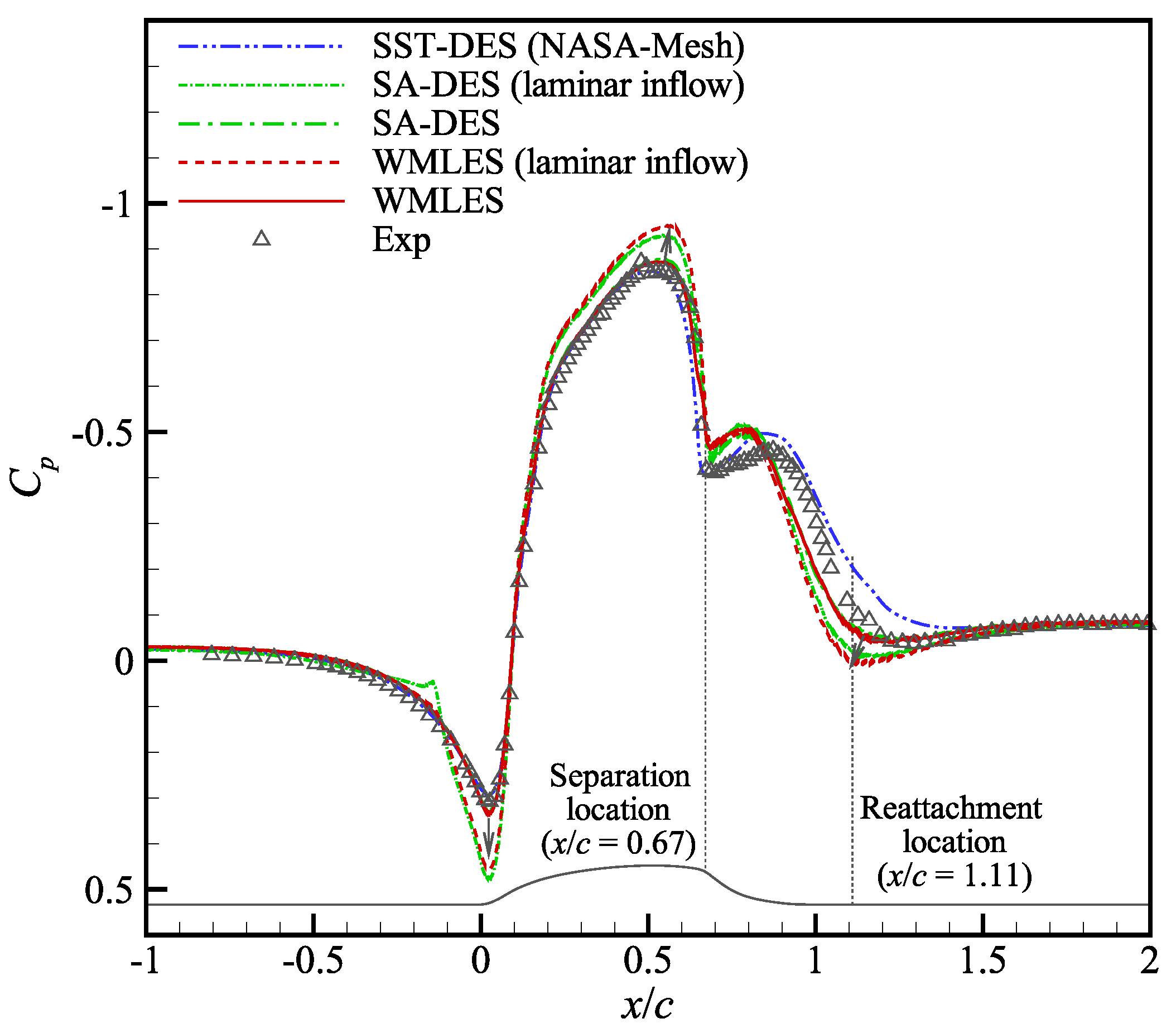
36] They have fully developed a turbulent boundary layer before flow separation, and even shock/boundary layer interference occurs. This study uses SA-DES, SST-DES and WMLES in OpenFOAM to simulate these three flows to assess the capability for various separated flows. The sensitivities of these methods to grid scale and turbulent inflow are also tested.
The work is organized as follows: In
Section 2, SA-DES, SST-DES and WMLES based on wall shear stress in OpenFOAM are described. In
Section 3, three flows over a circular cylinder, a wall-mounted hump and an axisymmetric bump and their physics models are introduced. In
Section 4, the simulation results of several WMLES methods on these three flows are compared. Conclusions are listed in
Section 5.
3. Physic Models
Three separation flows, including a flow over a circular cylinder at based on the diameter, a flow over a wall-mounted hump at based on the length of the hump, and a flow over an antisymmetric bump at and are simulated by the SA-DES, SST-DES and WMLES methods in OpenFOAM.
The computational domains for the three flows are a circular cylinder, a rectangle, and a wedge, respectively. Their geometric structure and computational domain are shown in
Figure 3. Their flow conditions are summarized in
Table 1. The computational domain and mesh structure for the cylinder case is consistent with the literature [
27] that presented the WRLES of the flow field. The spatial domain is
. The grid number is
1.44 million, which is one-fourth of the literature [
27].
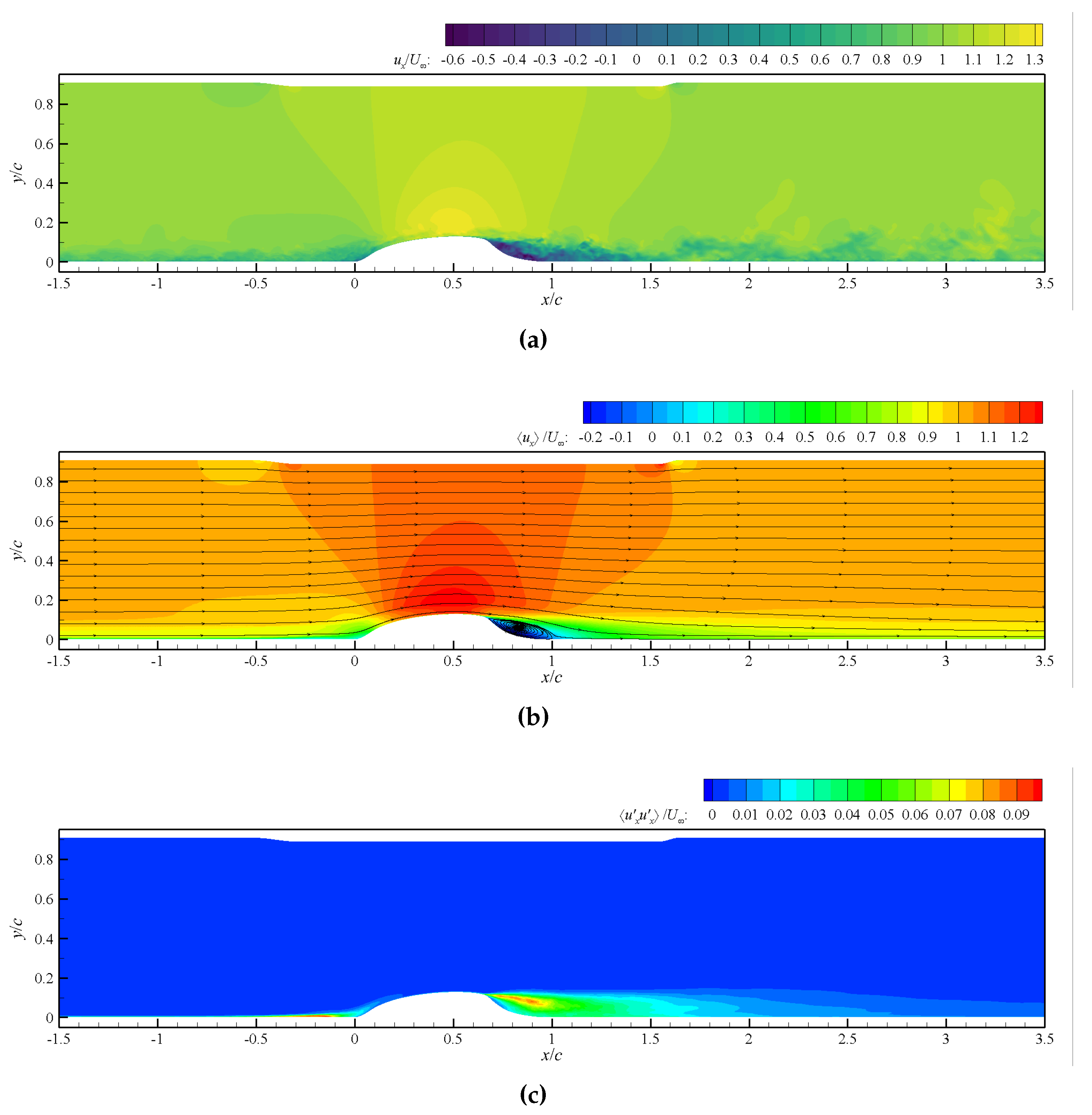
The length of the hump is
, and its height is
. The size of the computational domain corresponds to
Note the geometry is two-dimensional and does not vary in the span in the simulation. Here the same spanwise dimensions as Iyer and Malik [
38]. A contoured top wall is set upon the hump in the simulations based on the recommendations of the NASA CFDVAL2004 Workshop [
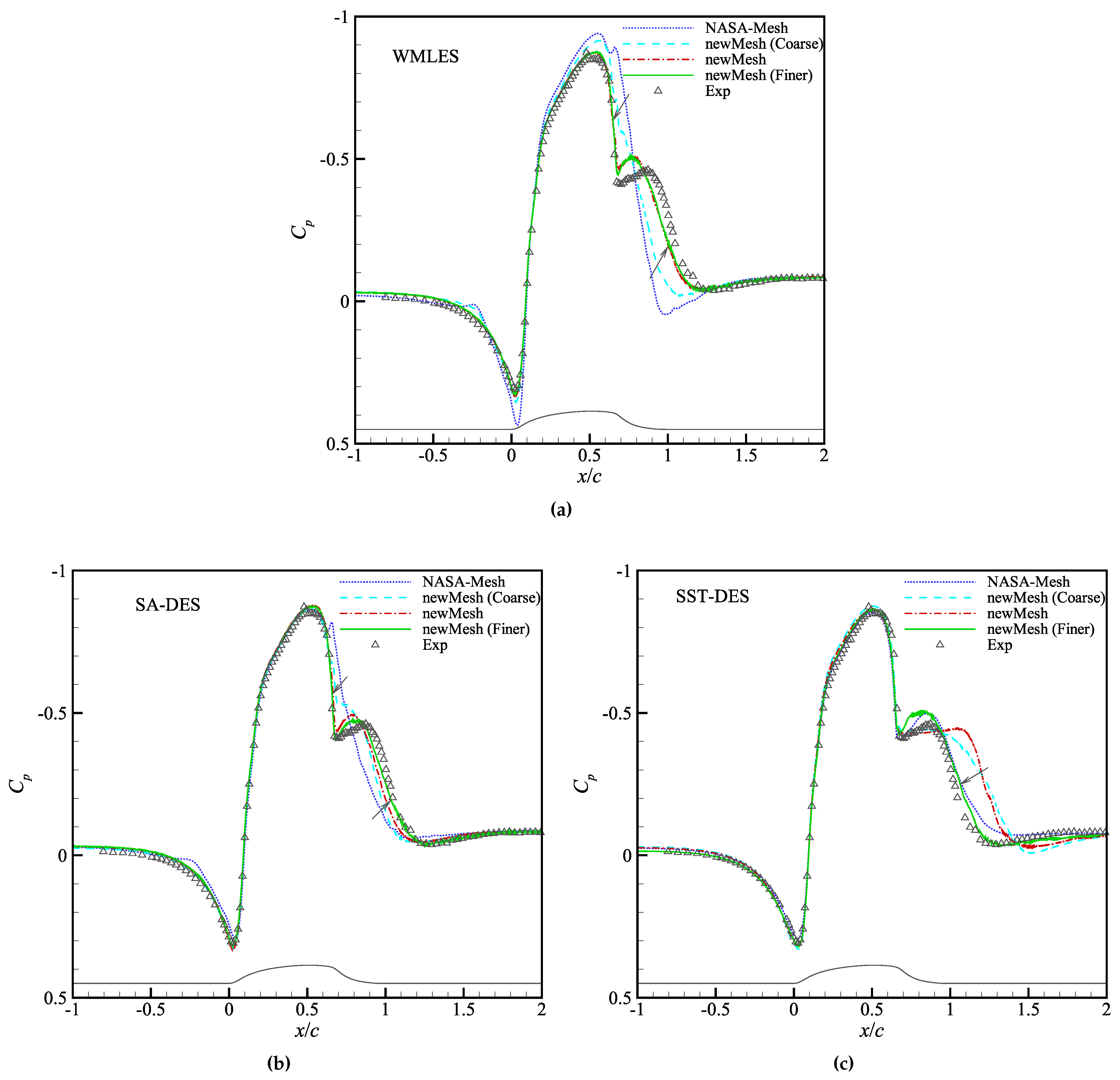
34] to account for the effect of the side-mounted end plates in the experimental test. Two grid systems are used for the wall-mounted hump case. The first gird is from the Turbulence Modeling Resource Web of Langley Research Center, and is defined as NASA-Mesh in
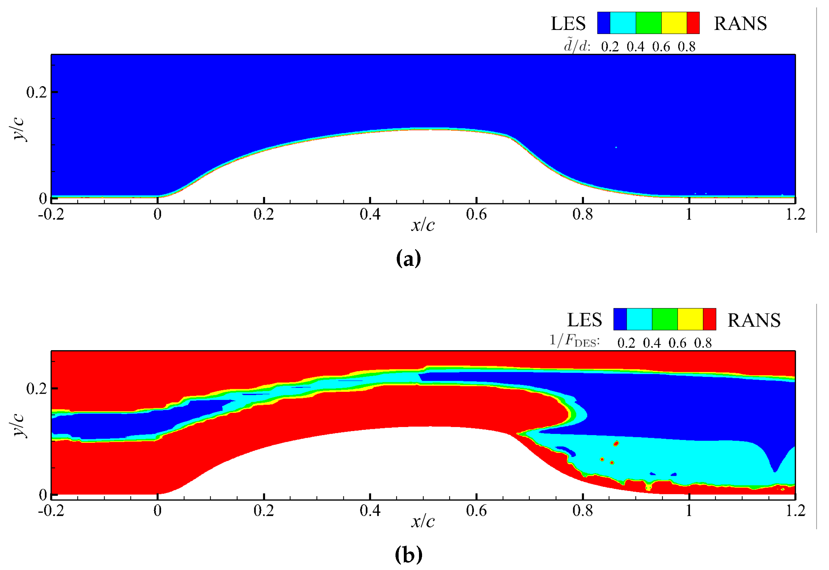
Figure 3. This grid has been verified to satisfy
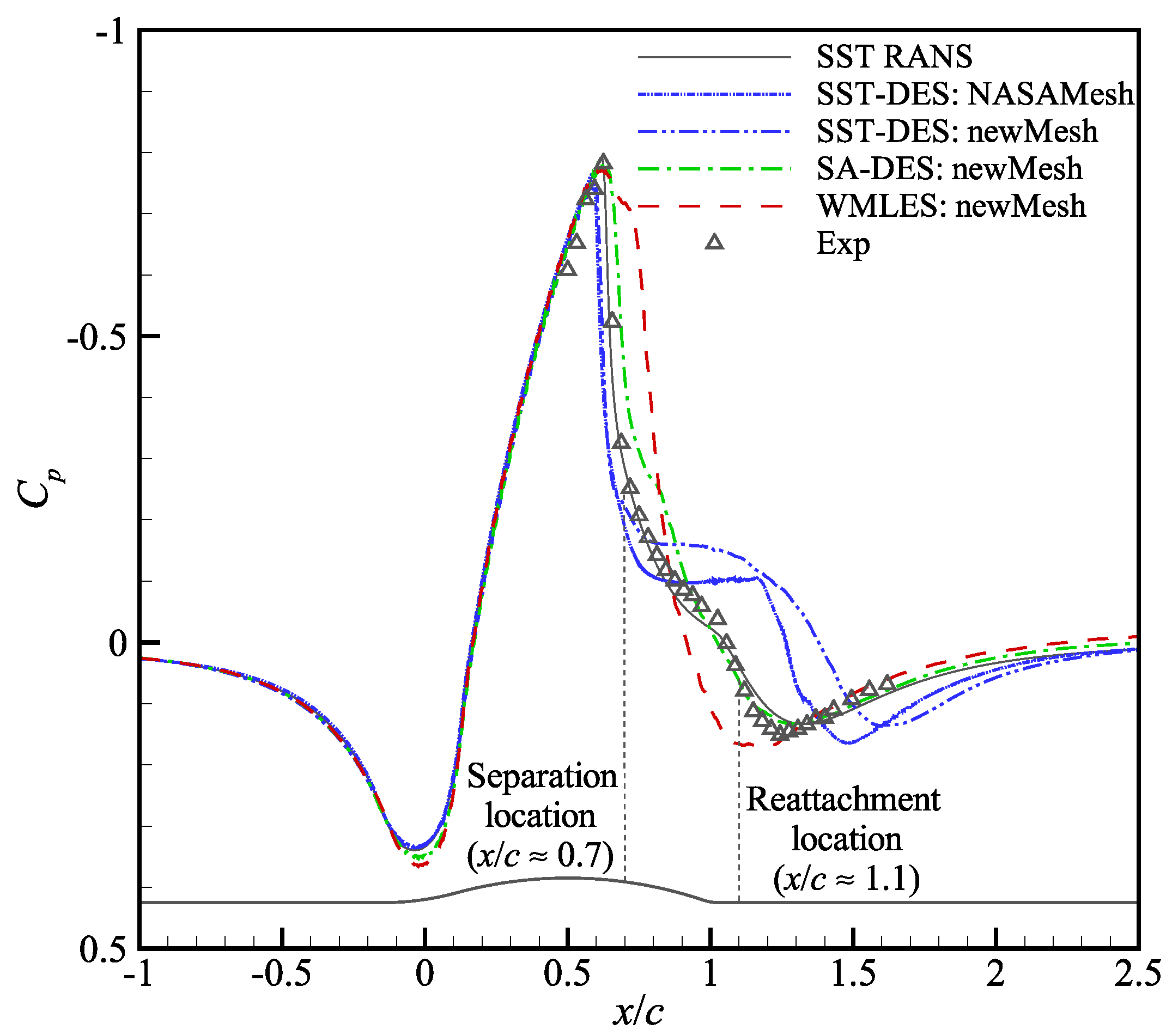
for various RANS models, but its streamwise grid size does not meet the requirements of LES. Another Cartesian grid system with prismatic boundaries is set for the wall-mounted hump case, namely NewMesh. Specific details and independent verification of NewMesh are detailed in the next section.
The transonic flow over an axisymmetric bump experiment of Bachalo et al. [
35] is simulated. The length of the bump is
. The domain consists of a 30° wedge with inner radius
and outer radius
. The bump height is
. This case also uses two grid systems similar to the wall-mounted hump case.
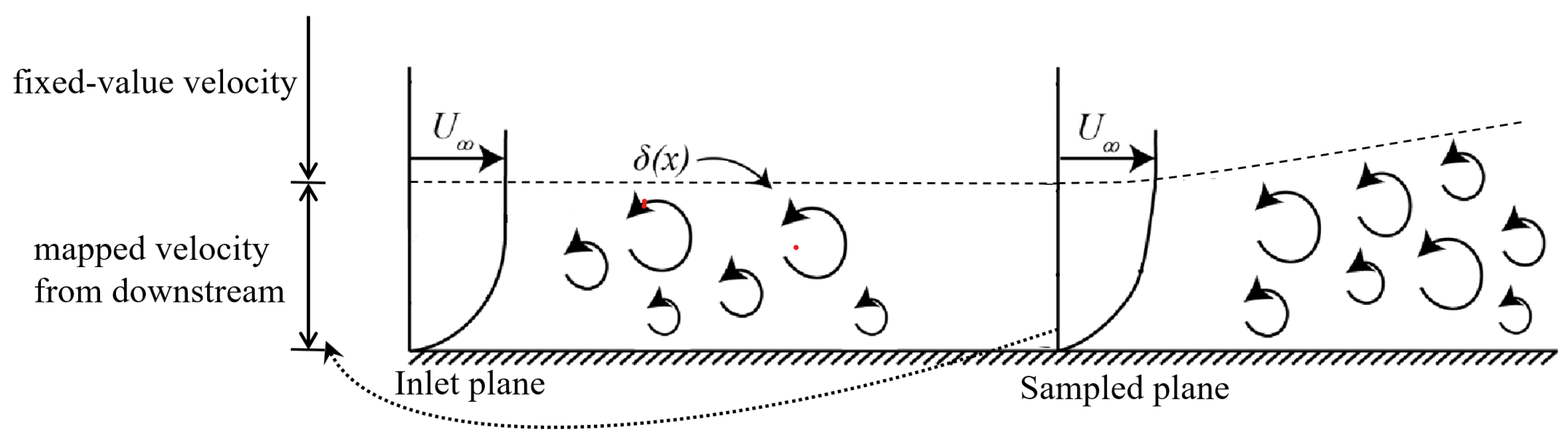
The first two cases have similar boundary conditions. A no-slip boundary condition is imposed for the velocity at the wall. The inlet boundary condition (on the left) is a fixed-value velocity with zero-pressure gradient, while the outlet boundary condition (on the right) adopts a wave transmissive boundary with a fixed-value pressure. The boundaries on both sides of the computational domain are periodic. The third case has different settings at the inlet and outlet. There is a fixed-value velocity, total temperature, and total pressure at the inlet boundary, while there is a zero-gradient velocity, temperature and pressure at the outlet boundary. Furthermore, the incoming flow of the latter two cases is divided into laminar incoming flow and turbulent incoming flow. For turbulent incoming flow, a composite setting is used at the inlet boundary, i.e., the velocities within the turbulent boundary layer are mapped directly from a certain distance downstream, while the upper layer velocities are directly set to a fixed value, as shown in
Figure 4.
5. Conclusions
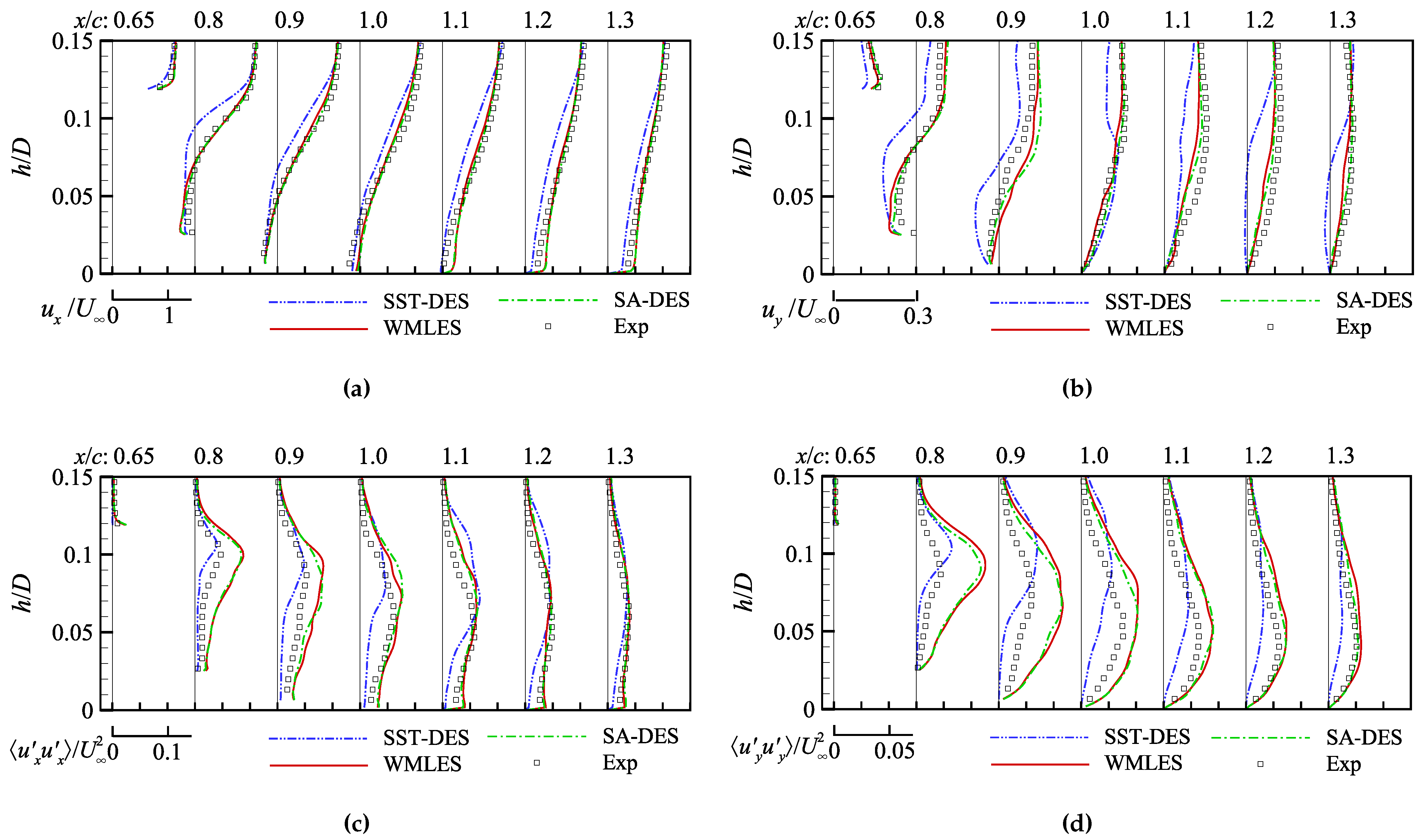
In this study, the WMLES, SA-DES, and SST-DES methods in OpenFOAM were tested on three separated flows, including flow over a cylinder at = 3900, separated flow over a wall-mounted hump at = 9.36 × 10⁵, and transonic flow over an axisymmetric bump with shock-induced separation at = 2.763 × 10⁶. The complexity of these three flows is gradually increasing. WMLES, SST-DES, and SA-DES methods in OpenFOAM can easily predict the separation position and wake characteristics in the flow around the cylinder, and they rely on the grid scale and turbulent inflow to accurately simulate the latter two flows.
In terms of grid independence, when the grid scales in the boundary layer meet the grid requirements proposed by Larsson et al. [
9] (
), it is possible to simulate the vortex structure in the turbulent boundary layer upstream of the flow separation. However, finer meshes are required to accurately predict the separation and reattachment. The second flow could be reproduced when using a three-level local-refined hexahedral mesh grid system with a near-wall grid scale of
. The third flow could be reproduced when using a four-level local-refined hexahedral mesh grid system with a near-wall grid scale of
. WMLES method is more sensitive to grid scales than the SA-DES method. The new grid constructed in this paper cannot meet the grid requirements of SST-DES, so its simulation results based on the structural grid system from NASA are closer to the experimental data.
Table 7 summarizes grid requirements for WMLES, SA-DES, and SST-DES in OpenFOAM.
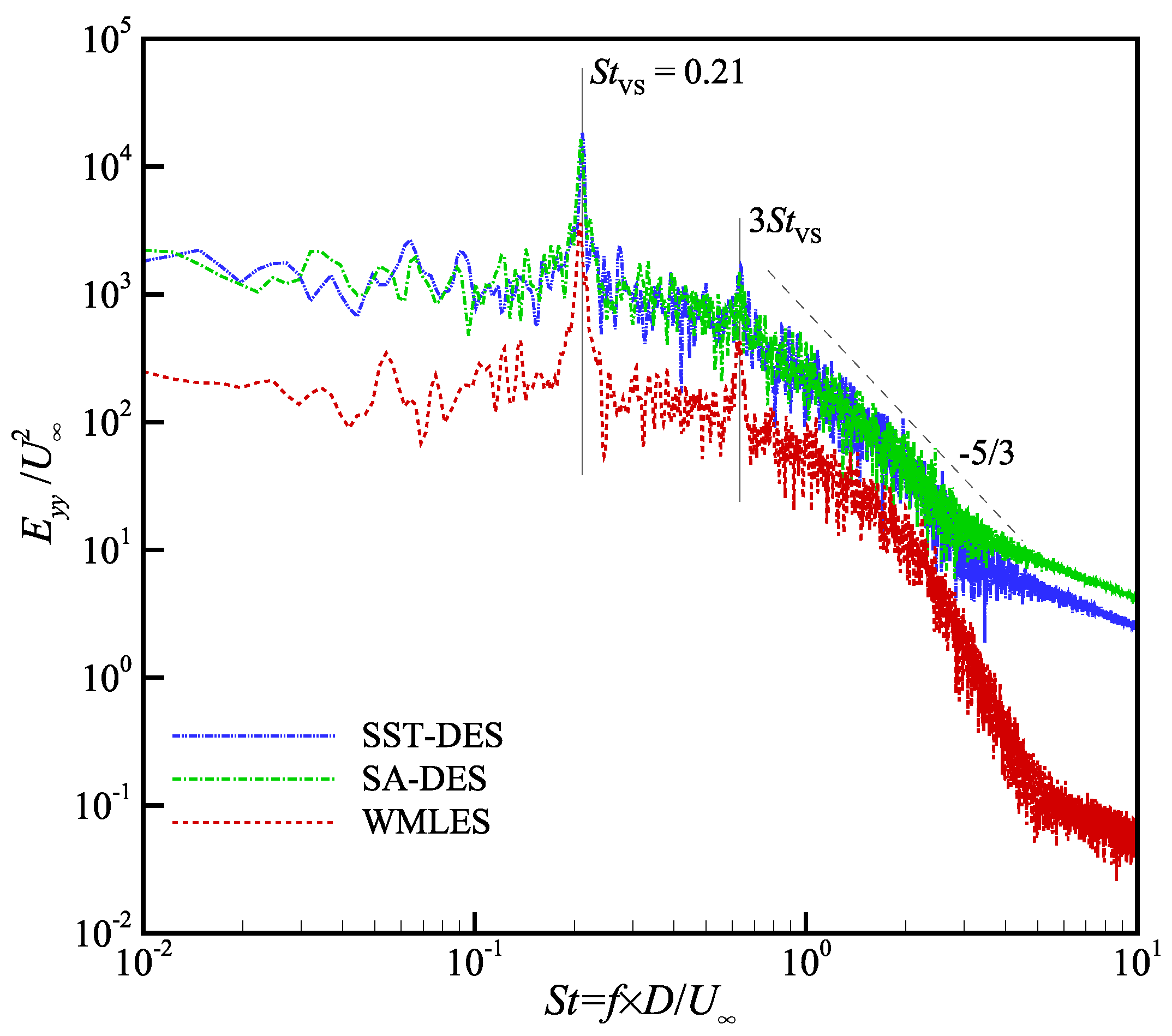
In terms of vortex description, SST-DES can only simulate vortices induced by the separated shear layer, while SA-DES and WMLES can also simulate vortices in the turbulent boundary layer upstream of the flow separation. Furthermore, WMLES with WALE and dynamic-k-equation SGS models and SA-DES can simulate the transition of the laminar boundary layer in the flow over the wall-mounted hump.


