Abstract
This paper gives a quantitative account of the influence of slipstream on the aerodynamic performance of a contrarotating propeller (CRP)/wing system, and compares it with the CRP and clean wing. To accurately evaluate the complex aerodynamic interaction, the unsteady Reynolds-averaged Navier–Stokes approach using the sliding mesh method is performed at a typical freestream velocity of 30 m/s. Four different critical parameters, including the freestream angle of attack (AoA), axial spacing between the front propeller (FP) and rear propeller (RP), number of blades, and rotational speed, are considered in the present work. The results show that the thrust coefficient, power coefficient, and propulsion efficiency of the CRP/wing system change sharply and the difference in amplitude between adjacent waves is large. In particular, the propeller slipstream has a significant impact on the lift–drag performance of the wing in the case of a nonzero AoA. The presence of a wing also increases the efficiency of propulsion due to the recovery of vortices. In the case of a small axial spacing, the thrust coefficient value of the FP is significantly smaller than that of the RP. However, when the axial spacing exceeds a certain value, the opposite relationship is obtained. When the rotational speed increases from 3695 RPM to 8867 RPM, the lift coefficient and drag coefficient of the wing gradually increase.
1. Introduction
Growing focus on reducing fuel consumption, protecting the environment, and improving the efficiency of propulsion has motivated the aerospace community to study the propulsion system of turboprop aircraft [1]. As a type of representative turboprop aircraft, a contrarotating propeller (CRP) aircraft has a higher efficiency and lower fuel consumption than a turbofan engine, which is technologically equivalent to it [2]. However, unsteady loads on the front propeller (FP) and rear propeller (RP) of the CRP system are more complex than those on an isolated rotating propeller (IRP), owing to periodic fluctuations. This phenomenon indicates that the slipstream created by the CRP, as well as the aerodynamic interactions between the CRP and wing, is more intense.
Considerable achievements have been attained over the last decade in determining the effects of the propeller slipstream on a wing, which have an important impact on the aerodynamic and structure design of turboprop aircraft. Most previous studies focused on the isolated propeller/wing interference in the case of a rigid wing [3,4,5]. When a propeller is placed in front of the wing, the slipstream it generates affects the lift–drag performance of the wing [6], increasing the lift-to-drag ratio [7] and stability control of the aircraft [8]. An approach based on the free-wake analysis was developed to analyzing the interference between the propeller and wings with different airfoils. The results showed the sensitivity of the thrust, power, and efficiency of aircraft to the conditions of the inflow and pitch of the blade, as well as wing airfoils [9]. However, the free-wake analysis requires correction factors to capture the influence of the slipstream on the wing. Cole et al. [10] proposed a higher-order free-wake approach to examine the interference in the propeller/wing system, where the wing and propeller blades were modeled as lifting surfaces with higher-order vorticity elements. Other studies investigated the benefits of the propeller/wing interactions, as well as the influence of the diameter of the propeller, its direction of rotation, and its position relative to the wing [10,11,12]. The wing influences the aerodynamic performance of the propeller by inducing velocity at its disk [9], developing a slipstream [5], and increasing the efficiency of the propulsion [9,13]. In addition to the rigid wing, there are also a few papers available that address the flexible wing in the propeller/wing system [14,15,16]. This research focused on the aeroelasticity phenomenon affected by the propeller.
For the CRP system, various researchers sought to predict the aerodynamic performance of the CRP, and a summary of this work is provided in [17,18]. Playle et al. used the fixed-pitch condition to emphasize the usefulness of the CRP configuration, but neglected the influence of radial interference on the FP [17]. This was proven to be unreasonable for the CRP, because complex interactions occur between the FP and RP [19]. Korkan obtained the planform and twist distribution of the FP and RP using a design segment of the method proposed by Playle et al., and analyzed the variable-pitch condition [19]. Stürmeri et al. [20,21] considered several approaches, e.g., PIV testing and a CFD simulation, to study the unsteady aerodynamic performance of the CRP and its noise reduction. The flow field exhibited a strong unsteadiness that was periodic, and was linked to the rotational speed and the number of blades (NoB) of the FP–RP. The overall unsteady loading of the RP was significantly reduced by alleviating the strength of the wake of the FP blades through trailing-edge blowing. The advantages at relatively low altitude were confirmed in an experimental study of the CRP for high-altitude airships, especially the higher efficiency over the IRP at various propeller advance ratios [22]. Compared with the IRP, the thrust of the FP reduced, but the thrust of the RP increased. Fiore et al. [23] performed a uRANS simulation and large eddy simulation to study the loss mechanisms in an 11 × 9 CRP configuration, and used the approach, cutback, and sideline operating conditions with the assumption of a phase lag to reduce computational costs. As in the full CRP configuration, they created swirl recovery vanes for the propulsion system of the propeller using the swirl in its slipstream to generate thrust to enhance its propulsive performance. However, the swirl recovery vanes were stationary [24,25]. They play a similar role in improving the efficiency of propulsion to that of a wing in the IRP/wing system or the CRP/wing system. In addition, the aerodynamic interaction between the FP and RP has a significant effect on the acoustics [26]. It can be concluded that the aerodynamic interference between the FP and RP in the CRP system is important because of its unsteady and rotational effects that complicate the surrounding flow field more.
To the best of our knowledge, there are few studies concentrated on the CRP/wing system, despite a wide body of research on the IRP/wing system and the CRP has been conducted. Addressing this is of primary importance for better understanding the CRP/wing aerodynamic interference caused by the slipstream to serve the CRP aircraft conceptual design. By using unsteady Reynolds-averaged Navier–Stokes (uRANS) equations based on the typical computational fluid dynamics (CFD) approach, this work quantifies the influence of four critical parameters—the freestream AoA, NoB, axial spacing between the FP and RP, and their rotational speeds—on the CRP/wing system, due to the slipstream of the CRP, through a comparison between the CRP/wing system and clean wing under identical computational conditions. Three values of axial spacing between the FP and RP are considered, with two sets of NoBs to design the CRP/wing system. In addition, this work can provide guidance for the conceptual design of aircraft, CRP aeroacoustic predictions, and the alleviation of structural vibrations.
The remainder of this paper is organized as follows: Section 2 provides the details of a series of geometric models for the CFD simulation, and Section 3 describes the specific numerical simulation strategy for the models, grid generation, test validation, and grid convergence study. In Section 4, the results of all the simulation cases using the four variables are illustrated and discussed, especially the influence of the slipstream of the CRP on the performance of the CRP/wing system. Finally, summaries of the CRP/wing system and the overall aerodynamic performance of the CRP configuration are provided in Section 5.
2. Model Description
To better understand the propeller slipstream, as well as the aerodynamic interaction between the propeller and the wing, a series of geometrical configurations were designed for the study. The clean wing geometry for the simulation was crucial for analyzing CRP/wing aerodynamic interferences. Figure 1a shows the geometry of a clean wing. The wing had a span length of 1 m and a chord length of 0.2 m (untwisted, unswept, and untapered). After trading the lift-to-drag ratio, zero-lift pitching moment coefficient, and stall angle, the wing airfoil EMX-07, whose profile is depicted in Figure 1b, was selected by referring to X-HALE [15] and multibody aircraft [27].
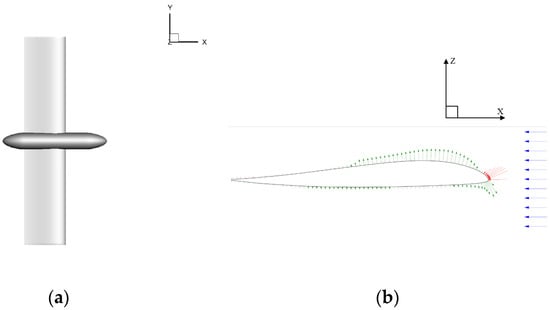
Figure 1.
Layouts of airfoil of the wing and airfoil: (a) clean wing; (b) EMX-07 airfoil.
The configuration of the IRP, shown in Figure 2a, consisted of two components. The main component was a propeller with four blades, denoted as 4-IRP. Similarly, a three-bladed propeller was used in the 3-IRP configuration. The second component of the IRP configuration was the nacelle, a fusiform body used to provide an aerodynamic surface for the propeller. The pitch angle of the blade was 25 deg at 70%R (R is the radius of the propeller). Viewed from the positive x-axis, the IRP rotated in a clockwise direction. The IRP/wing system shown in Figure 2b was constructed using an identical 1 m clean wing and the IRP configuration mentioned above. The center of the propeller was 0.568R from the leading edge of the wing. In this system, the nacelle could not only provide an aerodynamic surface, but also protect the payload mounted on the wing. Owing to the asymmetric airfoil EMX-07, the rotation axis of the propeller was not in the same plane as the plane of the chord of the wing.

Figure 2.
Layouts of the IRP and IRP/wing system: (a) IRP; (b) IRP/wing system.
Figure 3a shows the general layout of the CRP configuration obtained by installing a rear propeller behind the front propeller. Two different CRP configurations were used to validate the effects of the NoB, denoted with 3 × 3-CRP (three blades for the FP and three blades for the RP) and 4 × 4-CRP (four blades for the FP and four blades for the RP). To explore the influence of axial spacing between the FP and RP on the aerodynamic performance of the CRP, three values of axial spacing (0.24R, 0.44R, and 0.64R) were used. Similarly, from the front view, the FP rotated clockwise, and the RP rotated in the opposite direction. The CRP/wing system contained a 1 m clean wing and the CRP configuration, as shown in Figure 3b. We set a distance of 0.568R between the RP and the leading edge of the wing, and moved the FP forwards or backwards to obtain different axial spacings for the conceptual design and preliminary aerodynamic analysis. Two types of full CRP/wing configurations were used and denoted as 3 × 3-CRP/wing and 4 × 4-CRP/wing. Each configuration featured the three axial spacings of 0.24R, 0.44R, and 0.64R.
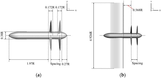
Figure 3.
Layouts of the CRP and CRP/wing systems: (a) CRP configuration; (b) CRP/wing system.
3. Computational Strategy
3.1. CFD Settings
The unsteady CFD computations of all the models were performed using Fluent, an unstructured, cell-centered commercial solver. The governing uRANS equations were used to describe the conservation of mass, momentum, and turbulent kinetic energy using the finite volume method through a pressure-based solver and a coupled pressure–velocity algorithm. The turbulence model that depended on a k-ω turbulence model with shear-stress transport (SST) was used together with an automatic wall function; the SST k-ω turbulence model has been used by other authors to evaluate the aerodynamic performance of propellers [19,22,28]. The least-squares cell-based method was used to compute the flow field gradients. All the numerical solutions were considered in a full three-dimensional and transient state. The user-defined function DEFINE_ZONE_MOTION was used to specify the rotating domain in the moving mesh simulation, which stabilized the calculation. To appropriately develop the propeller slipstream and propagate it well over and past the nacelle and wing, it was stipulated that the propeller would complete 10 revolutions. Moreover, the physical time step size corresponded to an azimuthal angle equal to 1 deg, as commonly reported in the literature [24,29]. There were, thus, 360 iterations per a full revolution of the propeller, with a maximum of 20 iterations in each time step. Subiterations within each time step reduced the residuals by at least five orders of magnitude, to enable the solution to converge.
The uRANS simulations were run on a workstation with the following metrics: 512 GB memory, 256 GB RAM, and 128 processors; they were initiated from the inlet condition. The boundary conditions for the entire simulation were as follows:
- The velocity inlet for the far field and inlet domain was established via the freestream AoA and freestream velocity of V∞ = 30 m/s. The corresponding Reynolds number based on the freestream velocity and a section of the blade of the propeller at r/R = 70% was 64,000.
- The condition of the pressure outlet was set at the domain of the outlet, where the magnitude of gauge pressure and pressure profile multiplier were set to default.
- Solid surfaces of the simulated geometry, including the propellers, nacelle, and wing, were modeled as a stationary wall with the no-slip shear boundary condition.
3.2. Grid Generation
Many advances were contributed to solving the unsteady Reynolds-averaged Navier–Stokes (uRANS) equations based on the typical CFD approach to analyze the slipstream of the propeller and the propeller/wing interactions [30,31]. Simulations of the propeller/wing interference could, in general, be divided into two main techniques. The first type was used to simulate the steady-state flow, which included the multiple reference frame (MRF) technique [32] and the actuator disk model [33], also known as the virtual blade model [34]. The other set of methods involved transient flow simulations, that is to state the methods considered the motion of the propeller at each time step, which contained the sliding mesh method (SMM) [28,35] and the overset mesh method (OMM) [36]. The SMM defined the similar computational domains to the MRF, with the difference being that the mesh and propeller rotated at each time step in the former, but were stationary in the latter. The OMM featured a background mesh and a component mesh that were generated independently. However, if the quality and density of the background mesh and component mesh did not match, orphan cells could have appeared in the calculation, having a substantial effect on accuracy. Since this work aimed to study the unsteady characteristics of the CRP/wing system and the requirements for the accuracy of the simulations, this analysis considered the classical SMM.
The SMM is a typical dynamic motion of the mesh, wherein the nodes move rigidly in a given mesh zone. The method was used to simulate the rotating motion of the IRP and CRP in this work. The SMM contained a stationary mesh domain and rotating mesh domains. A cylindrical computational domain was created for all simulation configurations, as shown in Figure 4a. There were two subdomains in the computational domain: a stationary domain, including the nacelle part and far field with, a sliding interface-out, adjacent to the out-body cell zone; and a rotating domain, enclosing the propeller with a sliding interface-in, adjacent to the in-body cell zone. The boundary of the interface was used to transfer the data between the stationary and rotating domains. For all the configurations, the whole simulation domain extended 12D upstream of the center of the propeller in the opposite streamwise direction. The outlet was placed at a distance of 36D away from the center of the propeller. The diameter of the far field was 25D. The size of the simulation domain could guarantee that the flow field around the blades was not perturbed by the boundary conditions. Figure 4b shows that a hybrid mesh was created, i.e., a static domain was generated by using structured elements (hexahedral elements) with an O-block technology, while the rotating domain surrounding the propeller was meshed using an unstructured mesh (tetrahedral mesh).
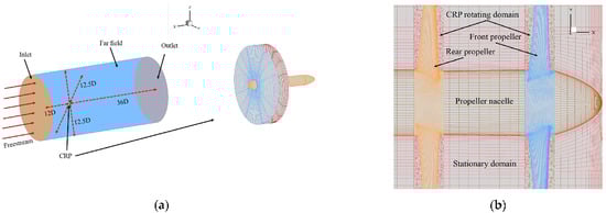
Figure 4.
SMM model: (a) cylindrical computational domain and two sliding cylindrical rotating domains for the CRP; (b) hybrid computational mesh.
The computational grids, displayed in this work, were generated using the ICEM CFD meshing software. There were 15 boundary layers on the prism grid adjacent to the surfaces of all the propellers and nacelles with a height ratio of 1.2. The surface meshes for the IRP, CRP, and entire computational domain are shown in Figure 5. The grid sizes for the different CRP and IRP configurations are listed in Table 1. In particular, the meshes of the leading and trailing edges and the tips of the blades required mesh refinements to improve the resolution of the flow simulation and capture details of the geometrical configuration, as shown in Figure 5c. The first grid layer spacing on the blade was 1 × 10⁻⁵ m, and y+ was less than 1.0. The same meshing strategy and mesh refinement were used for all the different geometry models investigated.
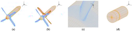
Figure 5.
Surface meshes: (a) IRP surface mesh; (b) CRP surface mesh; (c) mesh on the propeller root and hub; (d) mesh on the whole computational domain.

Table 1.
Grid sizes for different CRP and IRP configurations.
The meshes for the IRP/wing and CRP/wing configurations, shown in Figure 6, were significantly more complex than those for the isolated propeller and CRP. The grid sizes for the different CRP/wing and IRP/wing systems are summarized in Table 2. To ensure a sufficiently high resolution to determine the influence of the slipstream of the propeller on the wing, layers of hexahedral elements were resolved on the surface of the wing, with smaller elements arranged after the wing block.
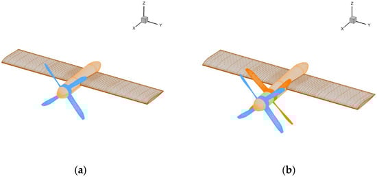
Figure 6.
Surface meshes for the IRP/wing and CRP/wing systems: (a) IRP/wing system; (b) CRP/wing system.
Table 2.
Grid sizes for different CRP/wing and IRP/wing systems.
3.3. Test Validation
A test case was chosen to evaluate the reliability and accuracy of the abovementioned grid generation method and computational strategy. As shown in Figure 7, the case was a typical rotor called the Caradonna–Tung rotor (C–T rotor), which has two blades in the shape of a rectangle [37]. The blades used an NACA 0012 profile and were untwisted and untampered. The radius of the rotor was 1.143 m, and the aspect ratio was 6. A collective pitch setting of 5 deg and a rotational speed of 1250 RPM were performed in this verification.
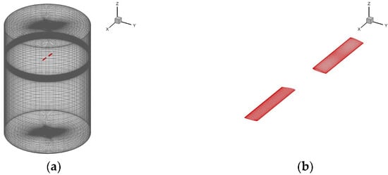
Figure 7.
Validation test case: (a) the whole computation domain; (b) mesh on the C–T rotor model.
The surface pressure coefficient distribution on five different sections (x/r = 0.50, 0.68, 0.80, 0.89, and 0.96) is displayed in Figure 8. cr is the length of the rotor chord and r stands for the rotor radius. The overall trends of the Cp for the present CFD simulation were consistent with the C–T rotor experimental data at the same location. As a result, it was convincing to use the grid generation method and computational strategy to evaluate the unsteady IRP and CRP aerodynamic performance.
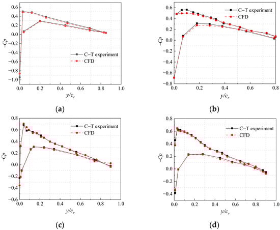

Figure 8.
Comparison of surface pressure coefficient distribution of C–T rotor in hovering state between experiment and CFD simulation: (a) x/r = 0.50; (b) x/r = 0.68; (c) x/r = 0.80; (d) x/r = 0.89; (e) x/r = 0.96.
3.4. Grid Convergence Study
To achieve high confidence in the grid generation and simulation strategy mentioned above, a grid convergence study was carried out for the four-bladed IRP configuration and the IRP/wing system, because modeling an IRP rather than the full CRP configuration allowed for a more careful addressal of the grid convergence issue. Table 3 presents the four grid sizes for the 4-IRP configuration and 4-IRP/wing system.
Table 3.
Different grid sizes for IRP configuration and IRP/wing system.
The propeller thrust coefficient, CT, torque coefficient, CQ, power coefficient, CP, and efficiency of propulsion, η, generated by the IRP and CRP, were calculated according to:
The power, P, could be measured in terms of n and Q as follows:
The advance ratio of propeller J was computed as follows:
In the above, T and Q represent the thrust and shaft torque of the propeller, respectively, both of which were obtained from the CFD simulation; P defines the power input to the propeller; ρ is the air density of the upstream flow; n and R represent the rotational speed and propeller radius, respectively.
The performance of the wing lift coefficient, CL, drag coefficient, CD, and pitching moment, CM, could be determined using:
where L, D, and M represent the lift, drag, and pitching moment of the wing, respectively; S represents the surface area of the wing; c denotes the chord length.
Table 4 shows the time-averaged coefficient of the propeller thrust, CTave, and propeller torque, CQave, at a high loading condition (J = 0.6) and a medium loading condition (J = 0.9). For the time-averaged force, the aerodynamic force was averaged over the last revolution. As the grid size decreased from G2 to G1, the errors in CTave and CQave became more significant compared with those when the grid size was increased from G2 to G4. At this setting, the aerodynamic performance of the IRP was the least sensitive to the grid size G2. The grids were acceptable in terms of the computational cost for all the configurations, and more refined grids would have been too computationally expensive. In Figure 9, a sketch is shown to explain the definition of the freestream AoA. The grid convergence study for the IRP/wing system was tested for AoA = 6 deg, by calculating the lift and drag coefficients as affected by the slipstream of the propeller. The results of the IRP/wing system were also gathered in Table 4. The numerical errors became negligibly small as the grid size increased from G6 to G8. In contrast, the numerical errors increased when the grid size decreased from G6 to G5.
Table 4.
Results of grid convergence study.
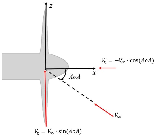
Figure 9.
Definition of angle of attack.
Figure 10 shows a comparison of the effects of the grid refinement on the field of the propeller slipstream for the distribution of the tangential velocity in a slice at X/R = 0.4, downstream of the propeller, and at X/R = 2.5, behind the wing, after five revolutions. Compared with the result for G5, a better fit was obtained for the remaining grid sizes in Figure 9a. However, for the distribution of axial velocity at X/R = 2.5, a maximum difference appeared near rc/R = 0.8 among the four sets of grid sizes (rc denoted). This might have occurred due to the rougher grid density behind the wing. It could be concluded that the grid scheme mentioned above could provide a sufficiently converged solution to use for the remainder of this work as well.
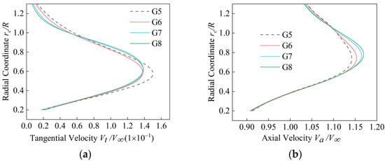
Figure 10.
Velocity distribution at different slice locations: (a) Vt distribution at X/R = 0.4: J = 0.6; (b) Va distribution at X/R = 2.5: J = 0.9.
4. Results and Discussion
In the following, we analyzed and discussed the computational results of the CRP and CRP/wing systems. The instantaneous propeller thrust and torque, lift of the wing, its drag, and pitching moment were written in separate files. The viscous forces and torque of the nacelle were not considered in the results of the propeller. The reference point for the coefficient of the pitching moment was located at a quarter of the chord length. Variations, including those in the AoA, FP–RP axial spacing, NoB, and rotational speed, were taken into consideration to better understand the overall aerodynamic performance of all the configurations. This provided a foundation for analyzing the aerodynamic characteristics of the CRP/wing system as influenced by the slipstream compared with the IRP/wing system and a clean wing. The performance of the propeller, including the FP, RP, and CRP, was assessed with the CT, CP, and η, while the performance of the wing was mainly assessed with the CL, CD, and lift-to-drag ratio. Accordingly, the clean wing and CRP were the cross-comparison models for the CRP/wing system when the four variations were altered. Note that all the evaluations presented here were based on a freestream velocity of V∞ = 30 m/s, which was the default setting for the aerodynamic measurements.
4.1. Effect of AoA
For nonaxial flow, the propeller wake geometry was changed, and the angle of the trailing vortices at the trailing edge of the blade was different from that in the case of the axial flow. In the case of a nonzero AoA or a gust for the CRP aircraft, which is a typical and common nonaxial flow condition, the performance of the propellers was much worthier being investigated under nonaxial flow circumstances. The models studied in this section are listed in Table 5. In Figure 11, the convergence of the CT, CP, and η curves showed that when AoA = 0 deg, the aerodynamic performance of the CRP exhibited remarkable cyclic fluctuations. This was because the RP was subjected to the unsteady, deflected inflow caused by the wake and tip vortices of the FP, and it, conversely, influenced the FP aerodynamic properties when the airflow passed by the RP. In contrast, the IRP was (quasi-)steady, because the angle between the pitch angle of any element of the blade and the inflow rarely changed when AoA = 0 deg. It could also be seen when AoA ≠ 0 deg, where the adjacent peaks in the aerodynamic curve were equal in magnitude, while the troughs were not in thorough equality, with the difference having increased slightly along with the AoA rising; this could be considered further for the structural fatigue load due to the fluctuation in the thrust coefficient.
Table 5.
The models studied when AoA was altered.
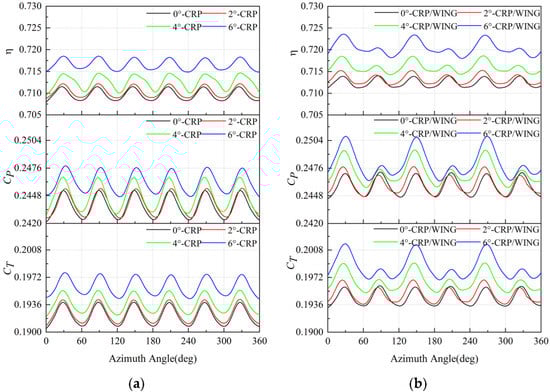
Figure 11.
Aerodynamic performance during a full revolution under different AoAs: (a) CRP configuration; (b) the CRP in CRP/wing system.
The unsteady aerodynamic performance of the CRP was periodic, as also shown in Figure 11. Within a certain range of the AoA, the aerodynamic coefficients of the full CRP configuration increased with the AoA. To better understand the influence of the wing on the CRP, a comparison of Figure 11a,b showed that the CRP/wing system improved the unsteady performance of the CRP substantially due to the existence of the wing. Six periodical oscillations appeared in every revolution, as well in this case. However, compared with the results of the CRP configuration, these oscillations in the CRP/wing system were more intense, and the difference in magnitude between the adjacent waves was larger. As the AoA increased, this difference became more obvious. When AoA = 6 deg, the curve of the CT in Figure 11b showed that the difference in magnitude between the adjacent waves was almost 24 times the value in Figure 11a, which meant that the influence of the wing on the aerodynamic performance of the propulsion system was critical.
To figure out how the wing affected the evolution of the propeller force, as the different oscillations appear in Figure 11b, the pressure distribution of the Y = 0.1 slice under different rotation azimuth angles (denoted with Ψ) is depicted in Figure 12. Although the distribution of the propeller pressure counter was similar in the CRP and CRP/wing configurations, the presence of the wing blocked the development in the propeller slipstream. As a result, a new higher pressure region was formed between the rear propeller and the wing, which led to an increment in the CRP thrust force in the CRP/wing configuration. It was also found that when Ψ changed from 0 deg to 90 deg, a stronger aerodynamic interaction was formed at Ψ = 30 deg, which corresponded to the maximum amplitude of the CT curve in Figure 11b. Therefore, it was observed that the two high-pressure regions grew closer, and the thrust force became larger.
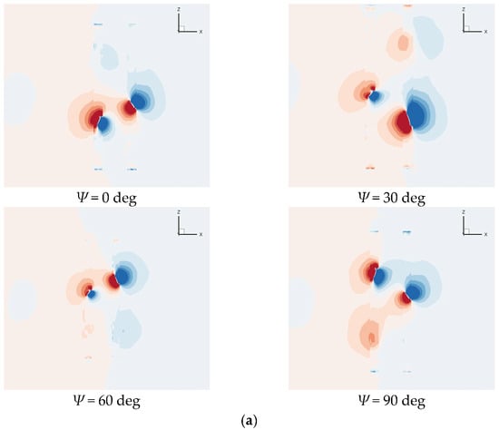
Figure 12.
Pressure distribution under different Ψ due to the CRP–wing interactions: (a) CRP configuration; (b) CRP/wing system.
To further quantifying the influence of the wing on the CRP, we set the time-average aerodynamic coefficients of concerning component in the CRP/wing system to normalize the values under different AoAs as Equations (6) and (7), with the relative values depicted in Figure 13. The results indicated that within 6 deg, the relative values were all greater than one, which showed that the time-averaged aerodynamic performance of the FP, RP, and CRP was positively influenced by the wing as the concerning values, as shown in Figure 13a,b. This was owing to the swirl recovery created by the wing. The aerodynamic performance of the FP, RP, and CRP increased along with the AoA rising, and the increment increased when the AoA was altered from 0 deg to 4 deg, then decreased from 4 deg to 6 deg. When the AoA became larger, the unsteady flow became more intricate, which would lead to a greater loading on the blade. It should be noticed that the value of the CTave of the FP in the CRP was greater than that of the RP, as Figure 13c shows, which appeared in the 4 × 4-CRP and 4 × 4-CRP/wing systems. The phenomenon was inconsistent with the former research, which was explained as the attribution to the FP slipstream absorbed by the RP. Based on this phenomenon, the axial spacing was taken into consideration to explore whether it was the reason behind this in the next section. In addition, the relative value when AoA = 4 deg was listed in Table 6, where the wing had the more positive and prominent impact on the RP, which could be attributed to the short distance between them in the CRP/wing system. Improvements in the efficiency of the propulsion of the FP, RP, and CRP were almost equal.
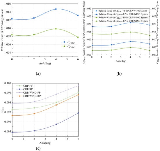
Figure 13.
Aerodynamic performance of FP, RP, and CRP under different AoAs: (a) relative value of CTave and CPave of CRP in CRP/wing system; (b) relative value of CTave and CPave of FP and RP in CRP/wing system; (c) real value of CTave of FP and RP in CRP configuration and CRP/wing system.
Table 6.
Relative changes in the aerodynamic performance of CRP and CRP/wing systems when AoA = 4 deg.
Moreover, Figure 14 shows the tendencies of the CL and CD in the 3 × 3-CRP/wing system and the IRP/wing system in one revolution when AoA = 6 deg. Three cyclic undulations appeared, which conformed with those of the IRP/wing system. This was also noted in the 4 × 4-CRP/wing system, which demonstrated that the fluctuation was only related to the number of blades of a single propeller. This was distinct from the features of the oscillation of the aerodynamic coefficients of the full CRP configuration in Figure 11. Based on the aerodynamic coefficients of the clean wing, the time-averaged aerodynamic performance of the wing (including the CLave, CDave, and lift-to-drag ratio) in the 3 × 3-CRP/wing system under four AoA settings was normalized as Equation (8) and depicted as Figure 15 shows. Values of the CLave and CDave in the same configuration increased with the AoA, which was consistent with the aerodynamic characteristics of aircraft. Indeed, the CRP in the CRP/wing system demonstrated a negative impact on the wing when AoA ≤ 2 deg, but the negative effect degraded, along with AoA increasing within 2 deg, which turned to the positive side when the AoA increased from 2 deg. When AoA = 4 deg, the CRP/wing system reached the optimal lift-to-drag ratio. This showed that the CRP system had a great impact on the lift of the wing under the flight state of the higher angle of attack, especially at the take-off and landing stages.
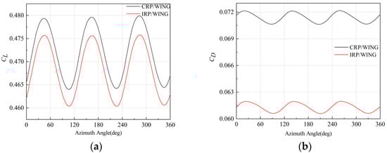
Figure 14.
Instantaneous lift and drag coefficient of wing in different systems: (a) CL; (b) CD.
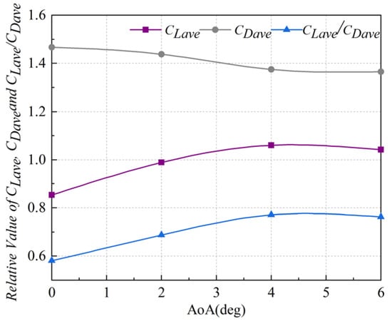
Figure 15.
Relative value of CLave, CDave, and lift-to-drag ratio when AoA was altered.
4.2. Effect of Axial Spacing between FP and RP
Due to the CTave of the FP in the CRP configuration being greater than that of the FP when the axial spacing was 0.64R, as shown in Figure 13c, and the importance of axial spacing, as in a CRP aircraft design variation, the influence of axial spacing between propellers on unsteady aerodynamic properties of the CRP and CRP/wing systems was evaluated in this section. The simulation conditions of the 4 × 4-CRP configuration and 4 × 4-CRP/wing system are shown in Table 7. A comparison of the time-averaged aerodynamic coefficients of the FP and RP and CRP in one revolution is shown in Figure 16a, as the spacing between the propellers varied. When the FP–RP axial spacing was 0.24R, the value of the CTave of the RP was 6.75% higher than that of the FP. As the axial spacing between the propellers increased, the value of the CTave of the FP gradually increased and, finally, exceeded that of the RP. This was because the RP was impacted by the flow field of the FP less severely as the axial spacing increased, which verified the speculation in Section 4.1. Accordingly, the energy assimilation of the RP from the FP was the critical factor for improving the RP’s aerodynamic performance. However, as the axial spacing increased from 0.24R to 0.64R, the influence of the interactions of the wake and tip vortices of the FP on the RP weakened, such that the coefficient of the thrust of the former tended to be equal to, or even greater than, that of the latter. As a matter of fact, the axial spacing of the CRP should have had greater importance attached to it, especially when the CRP was mounted on a wing compared with the property of a single propeller.
Table 7.
Simulation conditions when axial spacing varied.
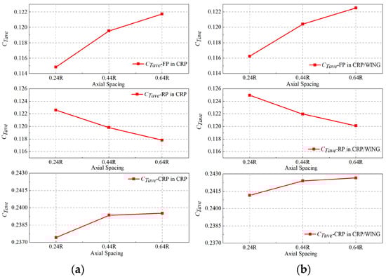
Figure 16.
Time-averaged CT performance affected by axial spacing: (a) CRP configuration; (b) CRP/wing system.
The corresponding thrust coefficients of the FP and RP and the CRP in the CRP/wing system are shown in Figure 16b, showing that they were significantly higher than those shown in Figure 16a. When the axial spacing was 0.24R, the value of the CTave of the FP increased to 1.21%, and that of the RP increased by 1.92%. They changed by 0.66% and 1.97%, respectively, when the axial spacing was 0.64R. On the one hand, the wing showed its positive impact on the FP, RP, and CRP in the CRP/wing system in regard to the aerodynamic property; on the other hand, compared with the impact of axial spacing, as the comparison in Figure 16a,b shows, the wing’s influence on the propeller was more significant when the axial spacing rose in the CRP.
To clearly illustrate how the axial spacing influenced the aerodynamic performance of the CRP and CRP/wing systems, Figure 17 shows the pressure distribution contours of the two configurations at Y = 0.0, with different axial spacings when the propeller rotated for six revolutions. As for the FP–RP axial spacing equaling to 0.24R, the low-pressure region between the front propeller and the rear propeller grew together, increasing the range of the low pressure. For the rear propeller, this meant that the pressure difference between the FP and RP became larger. In turn, due to the increase in the low-pressure range behind the propeller, the pressure difference of the FP was weakened, resulting in a decrease in the FP thrust force. Therefore, it could be explained why the CT of the RP reached the peak and the CT of the FP was minimum among the three axial spacing settings.
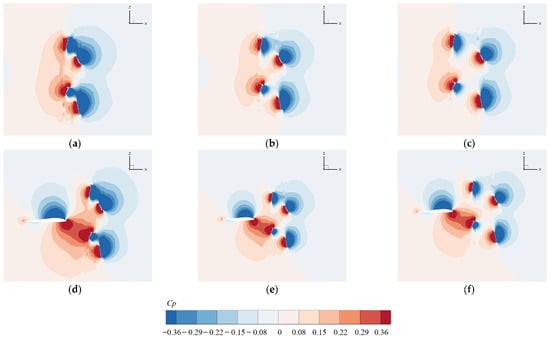
Figure 17.
Contours of pressure distribution on slices located at Y = 0.0: (a) 0.24R-CRP; (b) 0.44R-CRP; (c) 0.64R-CRP; (d) 0.24R-CRP/wing; (e) 0.44R-CRP/wing; (f) 0.64R-CRP/wing.
To assess the thrust coefficient, power coefficient, and efficiency of the propulsion of the CRP and CRP/wing systems with axial spacings of 0.24R, 0.44R, and 0.64R, Figure 18 depicts the results. When the axial spacing was 0.24R, the gaps in the peak values of the CT, CP, and η between the CRP in the CRP configuration and the CRP/wing system were 1.52%, 0.95%, and 0.52%, respectively, and 1.58%, 0.97%, and 0.56% when the axial spacing was 0.64R. The gaps indicated that within a reasonable range of axial spacing, the aerodynamic coefficients of the CRP/wing system were higher than that of the CRP without the influence of the wing. When the axial spacing was small, the amplitudes of the aerodynamic coefficients’ curves of the CRP configuration were equal. However, owing to the impact of the wing, the curves of the amplitude of the adjacent aerodynamic coefficients of the CRP in the CRP/wing system became inconsistent and fluctuated periodically in one revolution. Furthermore, the rising axial spacing balanced the unsteady performance and the aerodynamic property of the CRP in terms of the CT, CP, and η.
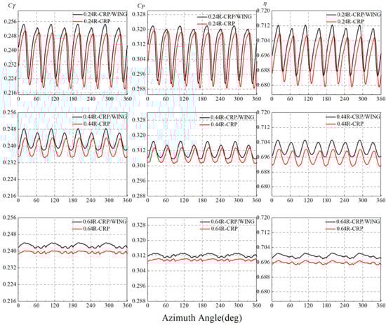
Figure 18.
A comparison of the aerodynamic performance of CRP in CRP configuration and CRP/wing system, with axial spacings of 0.24R, 0.44R, and 0.64R.
When the axial spacing was altered, it was necessary to assess the performance of the CRP/wing system, using not only the CRP performance, but also the wing performance, to figure out a value that was beneficial to both objects’ performance. Therefore, the performance of the wing in the CRP/wing system was the other aspect that needed to be taken into consideration.
The time-averaged values of the CL, CD, and CM of the wing in the 4 × 4-CRP/wing system during one rotation under the three axial spacings are shown in Table 8. The values of these variables gradually increased with the axial spacing. When the axial spacing increased from 0.24R to 0.64R, the values of the CLave, CDave, and CMave increased by 1.28%, 1.39%, and 17.20%, respectively.
Table 8.
Time-averaged coefficient of the CRP/wing system.
Figure 19a shows a comparison of the wing aerodynamic performance in transient and time-average forms, when the axial spacing between the propellers varied from 0.24R to 0.64R. When the axial spacing was 0.24R, the flow field of the slipstream was more intricate, owing to a more intense and unsteady aerodynamic interaction between the propellers. The aerodynamic performance curves fluctuated more intricately in this case, and the magnitude of the variations was lower than that of the axial spacing of 0.44R and 0.64R. As the axial spacing increased, the curves of the aerodynamic coefficients of the wing took a smooth form, indicating that the flow field was more stable. Accordingly, a small axial spacing meant that the airflow severely impacted the flow field surrounding the wing when it passed by its surface. Moreover, Figure 19c shows that the optimal aerodynamic performance of the wing in the three different axial spacings was in 0.44R.
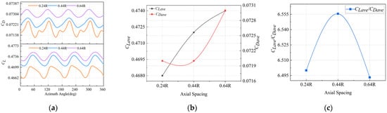
Figure 19.
Aerodynamic performance of the wing in CRP/wing system when the axial spacing varied from 0.24R to 0.64R: (a) instantaneous values of CL and CD in a full revolution; (b) time-averaged aerodynamic coefficients; (c) lift-to-drag ratio.
To determine the pressure distribution on the surface of the wing along the spanwise direction and the region influenced by the slipstream of the CRP, four different sections were selected, as shown in Figure 20a, where Y = −0.45 denotes the section near the root of the wing, Y = −0.1 represents the section on the radius of the half blade, Y = 0.2 marks the position along the edge of the semidiameter of the blade, and Y = 0.3 represents a section far from the root of the wing and outside the radius of the blade. Figure 20b,e show that the influence of the CRP with different axial spacings on the wing was almost equivalent when located outside the radius of the propeller. When they were located within the radius of the propeller, especially when Y = −0.1, a distinct magnitude of pressure distribution was obtained, as shown in Figure 20c. The distribution of pressure for the three different axial spacings at slice Y = −0.1 is shown in Figure 20f–h. Here, we could observe that there was a significant difference in the Cp distribution near the wing, except for the propeller region, which could explain that there was only a slight difference in the curve of the Cp in Figure 20c.
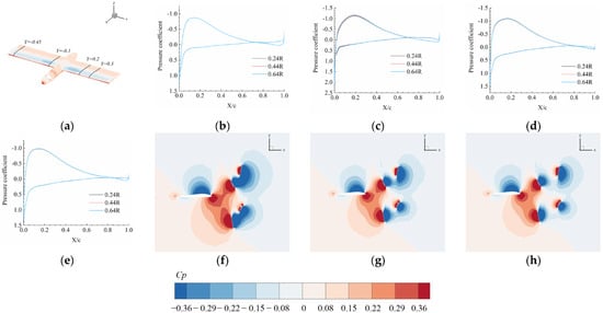
Figure 20.
Pressure distribution in the four sections and pressure contours: (a) four sections along the wing spanwise; (b) Y = −0.45; (c) Y = −0.1; (d) Y = 0.2; (e) Y = 0.3; (f) axial spacing = 0.24R; (g) axial spacing = 0.44R; (h) axial spacing = 0.64R.
4.3. Effect of NoB
Eight test cases in two different axial spacings were selected in the simulations to study the effects of the NoB on the aerodynamic performance of the CRP and CRP/wing systems. The configurations and flow conditions of each case are shown in Table 9.
Table 9.
Configurations and flow conditions of two test cases.
Table 10 shows the time-averaged aerodynamic coefficients of the CRP configurations with different NoBs when the axial spacing was 0.24R. The results showed that the number of blades had a substantial impact on the aerodynamic properties of the propeller. We set the 3 × 3-CRP as the baseline and added two blades to obtain the 4 × 4-CRP. The values of the CT and CP increased by 21.49% and 25.11%, respectively. It could be concluded that for the CRP with an axial spacing of 0.24R, the aerodynamic coefficients increased with the NoB. However, the greater the number of blades, the lower the efficiency of propulsion. This conclusion was also applicable to the CRP configuration with an axial spacing of 0.64R.
Table 10.
Time-averaged aerodynamic performance of CRP with different NoBs.
Table 11 shows the time-averaged aerodynamic coefficients of the CRP in the CRP/wing system with two sets of NoBs when the axial spacing was 0.24R. Compared with the results shown in Table 10, they showed that the wing improved the aerodynamic coefficients and the efficiency of the propulsion of the system. Because of the swirl recovery caused by the presence of the wing, the efficiencies of the CRP improved. Moreover, by setting the 3 × 3-CRP/wing system as the baseline, we found that the wing increased the value of the CTave of the 4 × 4-CRP/wing system by 22.13%, and that of the CPave by 25.66%, while the efficiency of the propulsion decreased. This tendency was also noted in configurations with an axial spacing of 0.64R.
Table 11.
Time-averaged aerodynamic performance of the CRP under different NoBs with the presence of a wing.
The unsteady loading of the FP and the RP in the CRP/wing system was periodic, as shown in Figure 21a,b. It could be concluded that the CT of the FP and the RP in the 3 × 3-CRP/wing system exhibited six cyclic fluctuations, i.e., the FP and RP passed each other six times per full revolution. Due to the effect of the blade passage, the aerodynamic performance of the 3 × 3-CRP fluctuated with a period of 6/rev. The fluctuations in the FP and RP were in phase, as in the 4 × 4-CRP/wing system. The number of fluctuations in every revolution was related to the number of FPs and RPs. This was the direct result as a consequence of the twice-per-revolution interactions of each blade in the FP with each RP blade, as discussed in [19]. Figure 21c displays the transient CL of the wing with the phase angle in one revolution when the axial spacing = 0.24R. As the phenomenon observed in Figure 14, the fluctuations were only related to the NoB of a single propeller in the CRP. The fluctuations were different from that of the FP and the RP of the CRP in the CRP/wing system, which were discussed in the following paragraph. A much stronger oscillation of CL was seen in the 3 × 3-CRP/wing system, because increasing the number of blades would distribute the blade loading more evenly. The more NoBs in a single propeller, the less unsteady aerodynamic properties behind it, because its layout was closer to the disk. Therefore, the wing’s CL of the 4 × 4-CRP/WING system was much smoother than that of the 3 × 3-CRP/WING system. When the axial spacing was 0.24R, the values of the CLave and CDave of the wing increased with the NoBs. However, the lift-to-drag ratio dropped when the NoB rose.

Figure 21.
Instantaneous unsteady loadings of the CRP and wing during a full revolution: (a) CT of FP and RP in 3 × 3-CRP/wing system; (b) CT of FP and RP in 4 × 4-CRP/wing system; (c) CL of wing in 3 × 3-CRP/wing system and 3 × 3-CRP/wing system.
Here, as mentioned in the discussion, the fluctuation frequency of the wing aerodynamic coefficient in one revolution was only related to the number of blades in a single-row propeller. The simulation results of the 3 × 3-CRP/wing system in one revolution were selected and the pressure contours were depicted every 60 deg by using Ψ as the variable to describe the pressure distribution in Y = 0.1 (as shown in Figure 20a). As shown in Figure 22, the pressure distributions along the leading edge of the wing, upper surface, and lower surface looped every one-third of a revolution, which meant that no matter what the initial phase angle between the FP and RP was, the influence of the CRP on the wing would loop every 120 deg. Therefore, for the 3 × 3-CRP/wing system, the CL and CD fluctuated three times, as shown in Figure 21c, which was applicable for the 4 × 4-CRP/wing system as well.
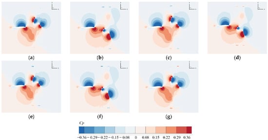
Figure 22.
Pressure distribution under different Ψ: (a) Ψ = 0 deg; (b) Ψ = 60 deg; (c) Ψ = 120 deg; (d) Ψ = 180 deg; (e) Ψ = 240 deg; (f) Ψ = 300 deg; (g) Ψ = 360 deg.
4.4. Effect of Rotational Speed
In ref. [24], the rotational speed influenced the aerodynamics of the propeller. The higher the rotational speed, the more distinct the effects of acceleration and the rotation of the wake of flow were. Accordingly, in this section, the aerodynamic performance of the CRP and the CRP/wing systems with an axial spacing of 0.44R was evaluated under six advance ratios (0.5, 0.6, 0.7, 0.9, 1.0, and 1.2) to figure out the disciplines and the optimal point. Due to the free stream velocity being maintained constant, in this section, the advance ratio means the same thing as the rotational speed, and the AoA was set to 6 deg.
The transient statuses of the CRP at different rotation speeds were different in the aerodynamic coefficients’ amplitude, while the fluctuation disciplines were identical, so there was no more detailed description. Additionally, the time-averaged outcomes were analyzed as follows, to illustrate the disciplines in general. The time-averaged coefficients, CTave, CPave, and the propulsion efficiency, η, of the CRP, and the CRP/wing systems are shown in Figure 23. This indicated the same tendency for each coefficient as the rotation speed varied, similar to that reported in the literature [22]. From this figure, although the CTave and CPave rose along with the rotation speed rising, the propulsion efficiency first increased and then decreased. The highest status appeared when the advance ratio was nearly 1.0, which depended on the characteristics of the propeller and the pitch angle. To highlight the CRP’s performance in the CRP/wing system with different advance ratios, their aerodynamic coefficients were normalized based on the outcomes of the CRP configuration, such as what Equation (6) indicated, and the results were depicted in Figure 24. For both the thrust and power performance, the performance of the CRP/wing system was lower than the CRP configuration when the advance ratio was lower than 0.6. To find out the reason, the performances of the FP and RP were analyzed.
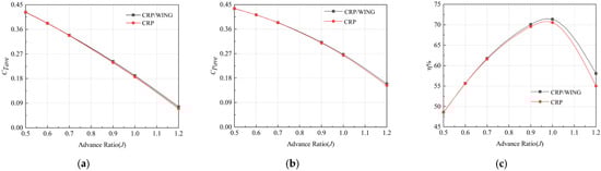
Figure 23.
Aerodynamic performance of the 4 × 4-CRP configuration and 4 × 4-CRP/wing system: (a) time-averaged thrust coefficient; (b) time-averaged power coefficient; (c) time-averaged propulsion efficiency.
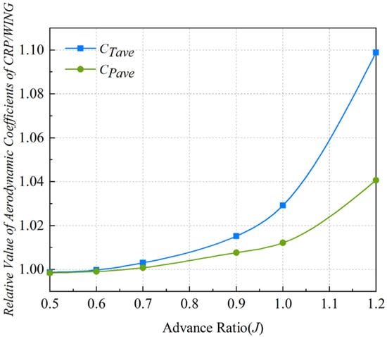
Figure 24.
Normalized CTave and CPave of CRP/wing system based on CRP configuration.
Figure 25 shows an aerodynamic performance comparison of the FP and RP in the CRP configuration and CRP/wing system at different advance ratios. Despite whether a wing was present or absent, the advance ratio had a considerable impact on the value of the CTave and CPave of the FP and RP, and both coefficients were in negative correlation with the advance ratio. Moreover, compared with the FP, the aerodynamic performance of the RP grew greater, along with the advance ratio decreasing. Due to the less intricate unsteady characteristics in the high advance ratio, the FP and RP operated without obvious interaction, and the interaction showed up when the advance ratio decreased. Figure 25c,f show the normalized aerodynamic coefficients of the FP and RP in the CRP/wing system based on the CRP configuration, as Equation (7) indicated. The bifurcation in Figure 25c indicated that the wing influenced the RP positively, more than the FP, along with the advance ratio rising. A possible explanation for this could lie in the shorter distance between the RP and the wing. However, when the advance ratio was lower than 0.6, the performances of both the FP and RP reached the same status, which indicated that the more intricate flow field caused by the high-speed-rotating propellers impaired the wing’s influence. Additionally, the aerodynamic interaction was mutual; therefore, the wing’s performance was analyzed next. It is worth noting that the rotational status at a higher advance ratio should be prioritized to prevent the propeller entering the “windmill” state.
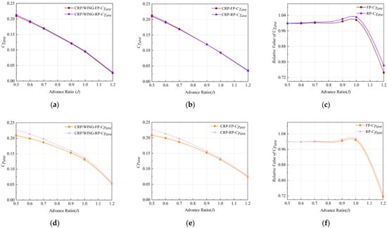
Figure 25.
Aerodynamic performance of the FP and RP with and without a wing: (a) CTave of FP and RP in the CRP/wing system; (b) CTave of FP and RP in the CRP configuration; (c) Relative Value of CTave of FP and RP in the CRP/wing system based on CRP configuration; (d) CPave of FP and RP in the CRP/wing system; (e) CPave of FP and RP in the CRP configuration; (f) Relative Value of CPave of FP and RP in the CRP/wing system based on CRP configuration.
Figure 26 shows the relationship between the aerodynamic performance of the wing in the CRP/wing system and the advance ratio. Figure 26a shows that the values of the CL and CD gradually improved when the advance ratio J decreased. However, the CL/CD in Figure 26a increased with the advance ratio, and it reached the maximum value at nearly J = 1.0; then, it started to decrease, which meant that the optimal performance of the wing appeared. The instantaneous values of the CL with different advance ratios in one revolution are shown in Figure 26b, indicating four fluctuations for each curve. At J = 0.5, and 1.2, for example, the magnitudes of CL varied by 0.18% and 0.02%, respectively, which showed that the impact of the slipstream of the CRP on the wing was more intense, and led to a greater variation in the magnitude of the CL when the propeller rotated at high speed.
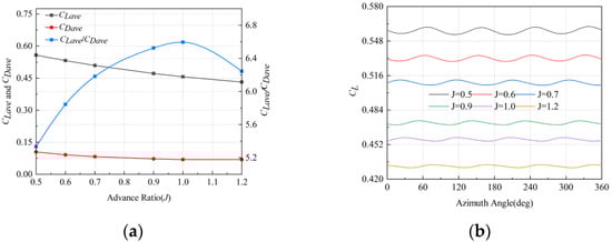
Figure 26.
Aerodynamic performance of the wing in 4 × 4-CRP/wing system: (a) CL, CD, and lift-to-drag ratio; (b) instantaneous value of CL at different advance ratios.
To further assess the influence of the slipstream, the profiles of the tangential velocity and axial velocity were exacted from the measurement slices at X/R = 0.4 (Figure 27a,d,g), X/R = 2.5 (Figure 27b,e,h), and X/R = 0.865, rc/R = 0.6 (Figure 27c,f,i) downstream of the center of the RP. Three conditions were selected to illustrate the influence of the advance ratio on the slipstream of the CRP; conditions involved a high loading, advance ratio = 0.5, an intermediate loading, advance ratio = 0.6, and a low loading, advance ratio = 1.2. In Figure 27a,d,g, Vt gradually reduced with the increase in the advance ratio. It could be concluded that, in the case of a high loading (Figure 27b) and an intermediate loading (Figure 27e), the presence of the wing reduced the axial velocity Va over most of the radial regions located at X/R = 0.56. The tendency was similar to that reported by Sinnige [24]. In that study, the installation of SRVs reduced Va. Figure 27c,f,i show that the distribution of Va in the spanwise direction at Y = −0.6 to 0.6 was affected by the slipstream of the CRP. The envelope of the CRP/wing system covered the CRP, which indicated that the wing had a positive influence on the slipstream of the CRP. Furthermore, this positive influence might have enhanced the lift of the wing. In the slipstream region, Va increased rapidly; we examined the peak at Y = 0.0 in the case of a large loading (Figure 27c, J = 0.5). However, for other loadings, the graph of Va had a dented area at Y = 0.0 regardless of the presence of the wing.
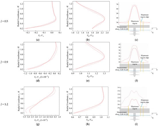
Figure 27.
Velocities of the slipstream of the 4 × 4-CRP and 4 × 4-CRP/wing systems (dashed line shows the 4 × 4-CRP/wing system and solid line shows the 4 × 4-CRP configuration): (a) Vt, in the case of a high loading (J = 0.5); (b) Va, in the case of a high loading (J = 0.5); (c) Va, in the case of a high loading (J = 0.5); (d) Vt, in the case of an intermediate loading (J = 0.9); (e) Va, in the case of an intermediate loading (J = 0.9); (f) Va, in the case of an intermediate loading (J = 0.9); (g) Vt, in the case of a low loading (J = 1.2); (h) Va, in the case of a low loading (J = 1.2); (i) Va, in the case of a low loading (J = 1.2).
5. Conclusions
In this paper, the influence of the unsteady aerodynamic interaction produced by a contrarotating propeller and wing was investigated. This was performed using variables such as the freestream angle of attack, FP–RP axial spacing, number of blades, and rotational speed. Based on the numerical results, it was shown that the sliding mesh method and numerical methods could predict the influence of the aerodynamic interaction of the CRP/wing system accurately. Different from the isolated propeller, the CRP configurations exhibited remarkable unsteadiness when the freestream AoA was 0 deg, due to interactions between the FP and RP. The CRP had a negative effect on the wing lift when the AoA was low. However, with the increase in AoA, the negative effect gradually disappeared, and the maximum lift-to-drag ratio was researched at 4 deg. Due to the presence of a wing, the difference in the amplitude of CT and CP and the propulsion efficiency η between the adjacent waves were statistically significant. Specifically, the greater AoA was, the larger the difference in the amplitude was, which indicated the more intricate aerodynamic interaction. Moreover, it was also shown that the axial spacing between the FP and RP had significant influence on the CRP/wing system aerodynamic performance; to be specific, the CTave of the FP and RP was altered when the axial spacing was altered. For instance, less axial spacing induced more intricate interference between the FP and RP, leading to a higher RP CT than that of the FP. The optimal axial spacing was nearly 0.44R, which provided the optimal lift-to-drag ratio for the wing. This was an important operating point for the aircraft conceptual design.
For each row propeller, the fluctuation frequency of the aerodynamic coefficients in one revolution occurred at twice the blade-passing frequency of the respective propeller in the other row. However, the wing aerodynamic coefficient fluctuation frequency in one revolution was only related to the number of blades in the single-row propeller. In addition, the comparison between the results of the CRP/wing system and CRP showed that the propulsion efficiency decreased as the NoB increased. It is worth noting that there was only a slight increase in the aerodynamic coefficients of the wing when using more blades, but the lift-to-drag ratio dropped when the NoB rose. When the free stream velocity remained constant, the value of the CTave and CPave decreased with the increase in the advance ratio, but this showed no relation to the wing. For the wing, the CL, and CD gradually improved when the advance ratio decreased. However, the lift-to-drag ratio did not change monotonously with the advance ratio, and reached the maximum value at J = 1.0. This advance ratio also corresponded to the most optimal working state of the propeller.
The current study showed a significant interference between the CRP and the wing under different designing variables. However, the conclusions were based on a fixed-blade pitch angle and same number of blades in a two-row propeller. Advanced research on the blade pitch angle and number of blades of two-row propellers may help to improve both the CRP and the aerodynamic performance of the wing.
Author Contributions
Conceptualization, C.X.; methodology, C.X. and Z.Z.; software, Z.Z.; validation, K.H.; formal analysis, Z.Z.; data curation, Z.Z.; writing—original draft preparation, Z.Z. and K.H.; writing—review and editing, C.X. and C.Y.; supervision, C.Y. All authors have read and agreed to the published version of the manuscript.
Funding
This research received no external funding.
Data Availability Statement
Not applicable.
Conflicts of Interest
The authors declare no conflict of interest.
Nomenclature
| Symbols | Definition |
| CRP | Contrarotating propeller |
| IRP | Isolated rotating propeller |
| FP | Front propeller |
| RP | Rear propeller |
| CFD | Computational fluid dynamics |
| uRANS | Unsteady Reynolds-averaged Navier–Stokes |
| MRFs | Multiple reference frames |
| SMM | Sliding mesh method |
| OMM | Overset mesh method |
| AoA | Freestream angle of attack, deg |
| NoB | Number of blades |
| RPM | Revolutions per minute |
| n | Rotational speed of propeller, rev/s |
| T | Propeller thrust, N |
| P | Propeller power, W |
| Q | Propeller torque, N · m |
| L | Wing lift, N |
| D | Wing drag, N |
| M | Pitching moment |
| CT | Thrust coefficient |
| CTave | Time-averaged thrust coefficient |
| CP | Power coefficient |
| CPave | Time-averaged power coefficient |
| CQ | Torque coefficient |
| CL | Lift coefficient |
| CLave | Time-averaged lift coefficient |
| CD | Drag coefficient |
| CDave | Time-averaged drag coefficient |
| CM | Pitching moment coefficient |
| CMave | Time-averaged pitching moment coefficient |
| CL/CD | Wing lift-to-drag ratio |
| Vt | Tangential velocity, m/s |
| Va | Axial velocity, m/s |
| J | Propeller advance ratio |
| V∞ | Freestream velocity, 30 m/s |
| R | Propeller radius, m |
| rc | Radial coordinate, m |
| r | C–T rotor radius, m |
| Cp | Pressure coefficient |
| c | Chord length, m |
| l | Span length, m |
| deg | Degree |
| Greek symbols | |
| η | Propulsion efficiency |
| ρ | Freestream air density, 1.225 kg/m3 |
| Subscripts | |
| ave | Time-averaged value |
| ∞ | Freestream value |
| a | Axial |
| t | Tangential |
References
- Benzakein, M.J. What does the future bring? A look at technologies for commercial aircraft in the years 2035–2050. Propuls. Power Res. 2014, 3, 165–174. [Google Scholar] [CrossRef]
- Strack, W.C.; Knip, G.; Weisbrih, A.L.; Godston, J.; Bradley, E. Technology and Benefits of Aircraft Counter Rotation Propellers; Techniacl Report, NASA Technical Memornadum 81232; NASA: Washington, DC, USA, 1981. [Google Scholar]
- Ferraro, G.; Kipouros, T.; Savill, A.M.; Rampurawala, A.; Agostinelli, C. Propeller-wing interaction prediction for early design. In Proceedings of the 52nd Aerospace Science Meeting, National Harbor, MD, USA, 13–17 January 2014. AIAA Paper 2014-0564. [Google Scholar]
- Aref, P.; Ghoreyshi, M.; Jirasek, A.; Satchell, M.J.; Bergeron, K. Computational study of propeller-wing aerodynamic interaction. Aerospace 2018, 5, 79. [Google Scholar] [CrossRef]
- Alba, C.; Elham, A.; German, B.J.; Veldhuis, L.L.M. A surrogate-based multi-disciplinary design optimization framework modeling wing–propeller interaction. Aerosp. Sci. Technol. 2018, 78, 721–733. [Google Scholar] [CrossRef]
- Bohari, B.; Borlon, Q.; Santos, P.B.M.; Sgueglia, A.; Benard, E.; Bronz, M.; Defoort, S. Conceptual design of distributed propellers aircraft: Non-linear aerodynamic model verification of propeller-wing interaction in high-lift configuration. In Proceedings of the 2018 AIAA Aerospace Science Meeting, Kissimmee, FL, USA, 8–12 January 2018. AIAA Paper 2018-1742. [Google Scholar]
- Veldhuis, L.L.M. Review of propeller-wing aerodynamic interference. In Proceedings of the 24th International Congress of the Aeronautical Science, Yokohama, Japan, 29 August–3 September 2014. [Google Scholar]
- Bouquet, T. Modelling the Propeller Slipstream Effect on the Longitudinal Stability and Control; Delft University Technology: Delft, The Netherlands, 2016. [Google Scholar]
- Marretta, R.M.A. Different wings flowfields interaction on the wing-propeller coupling. J. Aircr. 1997, 34, 740–747. [Google Scholar] [CrossRef]
- Cole, J.A.; Krebs, T.; Barcelos, D.; Bramesfeld, G. Influence of propeller location, diameter, and rotation direction on aerodynamic efficiency. J. Aircr. 2021, 58, 63–71. [Google Scholar] [CrossRef]
- Catalano, F.M. On the effects of an installed propeller slipstream on wing aerodynamic characteristics. Acta Polytech. 2004, 44. [Google Scholar] [CrossRef]
- Müller, L.; Friedrichs, J.; Kozulovic, D. Unsteady flow simulations of an over-the-wing propeller configuration. In Proceedings of the 50th AIAA/ASME/SAE/ASEE Joint Propulsion Conference, Cleveland, OH, USA, 28–30 July 2014. AIAA Paper 2014-3886. [Google Scholar]
- Kroo, I. Propeller-wing integration for minimum induced loss. J. Aircr. 2008, 23, 561–565. [Google Scholar] [CrossRef]
- Agostinelli, C.; Liu, C.; Allen, C.B.; Rampurawala, A.; Ferraro, G. Propeller-flexible wing interaction using rapid computational methods. In Proceedings of the 31st AIAA Applied Aerodynamic Conference, San Diego, CA, USA, 24–27 June 2013. AIAA Paper 2013-2418. [Google Scholar]
- Teixeira, P.C.; Cesnik, C.E.S. Propeller effects on the response of high-altitude long-endurance aircraft. AIAA J. 2019, 57, 4328–4342. [Google Scholar] [CrossRef]
- Hoover, C.B.; Shen, J.; Kreshock, A.R. Propeller whirl flutter stability and its influence on X-57 aircraft design. J. Aircr. 2018, 55, 2168–2174. [Google Scholar] [CrossRef]
- Playle, S.C.; Korkan, K.D.; Von lavante, E. A numerical method for the design and analysis of counter-rotating propellers. J. Propuls. Power. 1986, 2, 57–63. [Google Scholar] [CrossRef]
- Korkan, K.D.; Gazzaniga, J.A. Off-design analysis of counter-rotating propeller configurations. J. Propuls. Power. 1987, 3, 91–93. [Google Scholar] [CrossRef]
- Stürmer, A.; Marquez Gutierrez, C.O.; Roosenboom, E.W.M.; Schröder, A.; Geisler, R.; Pallek, D.; Agocs, J.; Neitzke, K.P. Experimental and numerical investigation of a contra rotating open-rotor flowfield. J. Aircr. 2012, 49, 1868–1877. [Google Scholar] [CrossRef]
- Stuermer, A. Unsteady CFD simulations of contra-rotating propeller propulsion systems. In Proceedings of the 44th AIAA/ASME/SAE/ASEE Joint Propulsion Conference & Exhibit, Hartford, CT, USA, 21–23 July 2008. AIAA Paper 2008-5218. [Google Scholar]
- Akkermans, R.A.D.; Stuermer, A.; Delfs, J.W. Active flow control for interaction noise reduction of contra-rotating open rotors. AIAA J. 2016, 54, 1413–1423. [Google Scholar] [CrossRef]
- Tang, Z.; Liu, P.; Chen, Y.; Guo, H. Experimental study of counter-rotating propellers for high-altitude airships. J. Guid. Control. Dyn. 2015, 38, 1491–1496. [Google Scholar] [CrossRef]
- Fiore, M.; Daroukh, M.; Montagnac, M. Loss assessment of a counter rotating open rotor using URANS/LES with phase-lagged assumption. Comput. Fluids 2021, 228, 105025. [Google Scholar] [CrossRef]
- Sinnige, T.; Stokkermans, T.C.A.; Ragni, D.; Eitelberg, G.; Veldhuis, L.L.M. Aerodynamic and aeroacoustic performance of a propeller propulsion system with swirl-recovery vanes. J. Propuls. Power. 2018, 34, 1376–1390. [Google Scholar] [CrossRef]
- Li, Q.; Öztürk, K.; Sinnige, T.; Ragni, D.; Eitelberg, G.; Veldhuis, L.; Wang, Y. Design and experimental validation of swirl-recovery vanes for propeller propulsion systems. AIAA J. 2018, 56, 4719–4729. [Google Scholar] [CrossRef]
- Kingan, M.J.; Parry, A.B. Acoustic theory of the many-bladed contra-rotating propeller: The effect of sweep on noise enhancement and reduction. J. Sound Vib. 2020, 468, 115089. [Google Scholar] [CrossRef]
- Meng, Y.; An, C.; Xie, C.; Yang, C. Conceptual design and flight test of two wingtip-docked multi-body aircraft. Chin. J. 2022, 35, 144–155. [Google Scholar] [CrossRef]
- Ruiz-Calavera, L.P.; Perdones-Diaz, D. CFD computation of in-plane propeller shaft loads. In Proceedings of the 49th AIAA/ASME/SAE/ASEE Joint Propulsion Conference, San Jose, CA, USA, 14–17 July 2013. AIAA Paper 2013-3798. [Google Scholar]
- Roosenboom, E.W.M.; Stürmer, A.; Schröder, A. Advanced experimental and numerical validation and analysis of propeller slipstream flows. J. Aircr. 2010, 47, 284–291. [Google Scholar] [CrossRef]
- De Rosa, D.; Morales Tirado, E.; Mingione, G. Paremetric invesgation of a distributed propulsion system on a regional aircraft. Aerospace 2022, 9, 176. [Google Scholar] [CrossRef]
- Ciliberti, D.; Nicolosi, F. Design, analysis, and testing of a scaled propeller for an innovative regional turboprop aircraft. Aerospace 2022, 9, 264. [Google Scholar] [CrossRef]
- Wang, H.; Gan, W.; Li, D. An investigation of the aerodynamic performance for a propeller-aided lift-enhancing double wing configuration. Aerosp. Sci. Technol. 2020, 105, 105991. [Google Scholar] [CrossRef]
- Zhang, Y.; Chen, H.; Zhang, Y. Wing optimization of propeller aircraft based on actuator disc method. Chin. J. Aeronaut. 2021, 34, 65–78. [Google Scholar] [CrossRef]
- Stajuda, M.; Obidowski, D.; Karczewski, M.; Józwik, K. Modified virtual blade method for propeller modelling. Mech. Mech. Eng. 2018, 22, 603–617. [Google Scholar] [CrossRef]
- Huang, Z.; Yao, H.; Sjögren, O.; Lundbladh, A.; Davidson, L. Aeroacoustic analysis of aerodynamically optimized joined-blade propeller for future electric aircraft at cruise and take-off. Aerosp. Sci. Technol. 2020, 107, 106336. [Google Scholar] [CrossRef]
- Chauhan, S.S.; Martins, J.R.R.A. RANS-based aerodynamic shape optimization of a wing considering propeller–wing interaction. J. Aircr. 2021, 58, 497–513. [Google Scholar] [CrossRef]
- Caradonna, F.X.; Tung, C. Experimental and analytical studies of a model helicopter rotor in hover. Vertica 1980, 5, 149–161. [Google Scholar]


Publisher’s Note: MDPI stays neutral with regard to jurisdictional claims in published maps and institutional affiliations. |
© 2022 by the authors. Licensee MDPI, Basel, Switzerland. This article is an open access article distributed under the terms and conditions of the Creative Commons Attribution (CC BY) license (https://creativecommons.org/licenses/by/4.0/).