Uncertainty Analysis of Parameters in SST Turbulence Model for Shock Wave-Boundary Layer Interaction

Abstract

Shock wave-boundary layer interactions (SWBLIs) have a tremendous influence on the performance of hypersonic vehicles. For the numerical simulation of such engineering flows, Reynolds averaged Navier-Stokes (RANS) still occupies an irreplaceable role. However, parameters of turbulence models in RANS have substantial uncertainties, which impact the reliability of simulation results. Thus, the aim of the present study is to conduct an uncertainty analysis on parameters in the shear-stress transport (SST) turbulence model for the simulation of SWBLIs. In the current work, uncertainty quantification was performed first. A surrogate model was constructed by the non-intrusive polynomial chaos (NIPC) method to propagate uncertainties from model parameters to the quantities of interests (QoIs) and quantify them. In the subsequent sensitivity analysis, the key parameters were identified for such flow by calculating the Sobol index of each parameter for various QoIs. The results indicate that uncertainties of model parameters led to non-negligible uncertainties in those QoIs, particularly in skin friction and wall heat flux. The parameters α₁, σ_ω1, β₁ were identified as primary contributors through the sensitivity analysis. Moreover, the specific effects of the three parameters on the flow prediction were analyzed by changing the parameters’ values separately.

1. Introduction

As the speed of vehicles constantly increases, shock wave-boundary layer interactions (SWBLIs) have been widely encountered in engineering and have a vital influence on the performance of supersonic and hypersonic vehicles. For example, the present of supersonic SWBLIs on the deflected control surface might influence the performance of this high-lift device. Chung et al. [1] studied the related simplified compressible swept convex-corner flow with different convex-corner angles and swept angles. They also installed a vortex generator at the corner to study its effect on SWBLIs [2]. The supersonic jet exhausts from the nozzle also involves a strong interaction between the shock wave and shear layer, and the fluidic injection method could diminish acoustic noise with less thrust penalty. Semlitsch et al. [3,4] identified the important design parameters in this control method and studied their influence on the evolution of shock patterns through numerical simulation. Moreover, Running et al. [5] experimentally investigated the global skewness and coherence of the hypersonic SWBLI in the cone/flare model, which is a typical configuration for high-speed aircrafts. Among the various forms of SWBLIs, the current study focused on separating the turbulent boundary layer induced by an incident shock wave, which typically exists in hypersonic inlets. The shock wave generated by the cowl lip may result in a large separation bubble near the inlet throat, causing the inlet to unstart and deteriorate its performance. Therefore, it is essential to perform in-depth research on this flow.

Since 1996, Schulein et al. have carried out a series of experiments regarding the interaction between an oblique incident shock wave and the turbulent boundary layer [6,7,8]. By continuously improving the measurement method, they provided vast experimental data, which were of great help to the validation of numerical methods. In terms of the numerical simulation for such flow, although the direct numerical simulation (DNS) and large eddy simulation (LES) methods have been extensively applied to basic studies alongside the improvement of computer power, the RANS method still plays a notable part in engineering applications due to its lower computation power requirements and sufficient robustness [9]. Therefore, enhancing the performance of the RANS method remains a research focus. It is well known that due to introduced assumptions and the lack of cognition of turbulence model parameters, the RANS method fails to acquire satisfactory results for the prediction of SWBLIs, particularly for wall heat flux after the reattachment of the separated boundary layer [10]. For deficiencies caused by introduced assumptions, many efforts have been undertaken. For instance, Steelant attempted to predict such flows using a turbulence model with compressibility corrections [11]. Fedorova et al. considered the influence of the incident shock-wave unsteadiness. Additionally, several researchers proposed that the overestimating of the wall heat flux was due to the failure of Morkovin’s hypothesis [12] at hypersonic Mach numbers, and the turbulent Prandtl number $P{r}_T$ could not be regarded as a constant. Xiao et al. [13] established additional transport equations related to enthalpy to achieve the variable $P{r}_T$, while Subhajit et al. [14] expressed $P{r}_T$ as a function of shock wave strength. Moreover, Lillard et al. [15] modeled the nonequilibrium effects in this flow by adding an additional equation. The studies mentioned above contributed to enhancing the behaviour of the turbulence models. However, instead of focusing on these flaws, the present study focused on the influence of uncertainty in turbulence model parameters caused by cognitive deficiencies.

The CFD Vision 2030 Study [16] indicated that the uncertainty in turbulence models and the lack of error management were limitations for further implementing the RANS method in engineering problems. In the process of putting forward the RANS method, several assumptions, experiences, and analogies were introduced [17], making the method more practical (but also more uncertain). Xiao [18] classified the uncertainties of RANS into four categories, amongst which the most direct was the parameters’ uncertainty in the turbulence model. At the initial period, the parameters were determined through fundamental and canonical experiments. The errors of measurements and the inadequacy of physical cognition resulted in the uncertainty of parameters. Moreover, as the flows become increasingly complicated, such as SWBLIs and other flows with strong nonequilibrium characteristics, the reliability of simulations utilizing the turbulence model with original standard values may be questioned. Taking the parameter $a_1$ in the SST turbulence model [19] as an example, its standard value is 0.31, derived from the log layer in the turbulent boundary layer. However, Matyushenko [20] diminished its value to 0.28 to accurately predict airfoil characteristics with a high Reynolds number near stall. In the simulation of the separation vortex flow in a circular tube, the parameter $a_1$ was adjusted to 0.3255 to reconcile the results with the experimental data [21]. These studies illustrated that the model’s parameters were variable over an uncertain interval rather than fixed. Nevertheless, the consequences in the numerical results resulting from the parameters’ uncertainties are rarely estimated in engineering, causing the results to lack credibility and restricting the further development of turbulence models. At a NASA symposium held in 2017 [9], uncertainty analysis, particularly uncertainty quantification, was identified as a future direction of turbulence modeling. Thus, it is vital to execute an uncertainty analysis on the turbulence model’s parameters.

Uncertainty analysis, which belongs to the realm of probability statistics, has been commonly employed in product design in the industry, and was just initially applied to the study of turbulence models to investigate the influence of turbulence models’ uncertainties on the results of the numerical simulations. To achieve this end, a surrogate model was constructed to propagate uncertainty from the parameters to QoIs (such as wall pressure) and to calculate the standard deviation and uncertainty interval for the QoIs. In recent years, several related studies have been conducted. Hosder et al. [22,23,24] performed a series of works for different turbulence models in various flows, including transonic wall-bounded flows, compression ramp flows, and relatively complex engineering problems. They quantified the effects of uncertainties in the model’s parameters for different QoIs and identified the key parameters through sensitivity analysis. Zhao et al. [25] analysed the parameters’ uncertainty for predicting wall heat flux in hypersonic flows over the double-ellipsoid model and X-33 flight vehicle. Moreover, based on uncertainty analysis, Subbian et al. [26] applied Bayesian inference to calibrated parameters in the correction terms of the SST turbulence model for complex vortical flows and Li et al. [27] also utilized Bayesian inference to calibrate the parameters in the Spalart-Allmaras (SA) turbulence model in a jet flow and assessed the model’s error. These studies established a firm basis for further uncertainty analysis on turbulence models and following works.

In the current study, we carried out uncertainty analysis on the SST turbulence model’s parameters for a two-dimensional turbulent boundary layer separation that was induced by an oblique incident shock wave with different interaction degrees. First, the influence of the parameters’ uncertainties on the prediction results was quantified using the NIPC method. Then, sensitivity analysis with the Sobol index was performed to identify the key parameters primarily responsible for the uncertainties in the results. Furthermore, the specific influence of the key parameters on the flow prediction was analyzed. The layout of this paper is arranged as follows. Section 2 introduces the SST turbulence model, the methodology involving uncertainty analysis, and the computational details. In Section 3, the prediction performance of the SST turbulence model in SWBLIs is evaluated first, and then the results of uncertainty quantification and sensitivity analysis are presented and discussed. Finally, Section 4 summarizes the main conclusions.

2. Methods and Computational Details

2.1. SST Turbulence Model

The SST turbulence model was initially put forward by Menter [19] in 1994. By introducing a blending function, the model realized the transformation from using the k–ω model near the wall to employing the k–ε model far away from the wall. In this way, the SST model could no longer require complex treatments for the region near the wall and avoid the deficiency of over-sensitivity to incoming flows. Meanwhile, Menter considered Bradshaw’s hypothesis in calculating turbulent eddy viscosity, which effectively improved the model’s performance for simulating the flows with strong unfavorable pressure gradients. Therefore, the SST model has become one of the most commonly used method in engineering. Its specific form is

$$\frac{\partial (\rho k)}{\partial t}+\frac{\partial (\rho u_{j}k)}{\partial x_j}=P_1-{\beta }^{\ast }\rho \omega k+\frac{\partial }{\partial x_j}\left[(\mu +{\sigma }_k{\mu }_t)\frac{\partial k}{\partial x_j}\right],$$

(1)

$$\frac{\partial (\rho \omega )}{\partial t}+\frac{\partial (\rho u_j\omega )}{\partial x_j}=\frac{\rho \gamma }{{\mu }_t}{P}_1-\beta \rho {\omega }^2+\frac{\partial }{\partial x_j}\left[(\mu +{\sigma }_{\omega }{\mu }_t)\frac{\partial \omega }{\partial x_j}\right]+2\left(1-F_1\right)\frac{\rho {\sigma }_{\omega 2}}{\omega }\frac{\partial k}{\partial x_j}\frac{\partial \omega }{\partial x_j}$$

(2)

The term of production $P_1$ is calculated as

$$P_1={\tau }_{ij}\frac{\partial u_i}{\partial x_j}, {\tau }_{ij}={\mu }_t(2S_{ij}-\frac{2}{3}\frac{\partial u_k}{\partial x_k}{\delta }_{ij})-\frac{2}{3}\rho k{\delta }_{ij}, S_{ij}=\frac{1}{2}(\frac{\partial u_i}{\partial x_j}+\frac{\partial u_j}{\partial x_i}),$$

(3)

where ${\mu }_t$ is the turbulent eddy viscosity, expressed as

$${\mu }_t=\frac{\rho a_{1}k}{\max (a_1\omega ,\Omega F_2)},$$

(4)

The parameter $a_1$ is derived from Bradshaw’s hypothesis, which proposes that the turbulent shear stress is proportional to the turbulent kinetic energy k:

$${\tau }_{\mathrm{ij}}=\rho a_{1}k.$$

(5)

The model’s parameters are calculated as

$$\varphi =F_1{\varphi }_1+(1-F_1){\varphi }_2, \left(\varphi =\beta ,{\sigma }_k,{\sigma }_{\omega },\gamma \right),$$

(6)

where ${\varphi }_1$ and ${\varphi }_2$ represent the parameters stemming from the original k–ω model (${\beta }_1,{\sigma }_{k1},{\sigma }_{\omega 1},{\gamma }_1$) and the transformed k–ε model (${\beta }_2,{\sigma }_{k2},{\sigma }_{\omega 2},{\gamma }_2$), respectively. Among them, the parameters ${\gamma }_1$ and ${\gamma }_2$ are regard as the scaling coefficients between the production terms of k equation and ω equation, which can be calculated by other parameters. The specific expression is as

$${\gamma }_1=\frac{{\beta }_1}{{\beta }^{\ast }}-{\sigma }_{\omega 1}\frac{{\kappa }^2}{\sqrt{{\beta }^{\ast }}}\begin{array}{cc},& {\gamma }_2=\frac{{\beta }_2}{{\beta }^{\ast }}-{\sigma }_{\omega 2}\frac{{\kappa }^2}{\sqrt{{\beta }^{\ast }}}\end{array}.$$

(7)

The blending function $F_1$ used for transformations between the two models is equal to one near the wall and drops to zero away from the wall. The blending functions $F_1$ and $F_2$ are given by

$$\begin{array}{c}{F}_1=\tanh ({\Gamma }^4)\\ \mathsf{\Gamma }=\min [max({\mathsf{\Gamma }}_1,{\mathsf{\Gamma }}_3),{\mathsf{\Gamma }}_2]\\ {\mathsf{\Gamma }}_1=\frac{500\mu }{d^2\omega \rho },{\mathsf{\Gamma }}_2=\frac{4\rho {\sigma }_{\omega 2}k}{d^2(C{D}_{k-\omega })},{\mathsf{\Gamma }}_3=\frac{\sqrt{k}}{{\beta }^{\ast }\omega d}\\ C{D}_{k-\omega }=\max \left(2\rho {\sigma }_{\omega 2}\frac{1}{\omega }\frac{\partial k}{\partial x_i}\frac{\partial \omega }{\partial x_i},{10}^{-20}\right),\\ F_2=\tanh \left({\mathsf{\Pi }}^2\right),\mathsf{\Pi }=\max \left(2{\mathsf{\Gamma }}_3,{\mathsf{\Gamma }}_1\right)\\ \mathsf{\Omega }=\sqrt{2W_{ij}{W}_{ij}},W_{ij}=\frac{1}{2}\left(\frac{\partial u_i}{\partial x_j}-\frac{\partial u_j}{\partial x_i}\right)\end{array}$$

(8)

where $d$ is defined as the shortest distance to the wall.

Table 1. Standard values of parameters in the SST model with uncertainty boundaries.

Parameter	Standard Value	Lower	Upper
${\sigma }_{\omega 1}$	0.5	0.3	0.7
${\sigma }_{\omega 2}$	0.856	0.7	1.0
${\sigma }_{k1}$	0.85	0.7	1.0
${\sigma }_{k2}$	1.0	0.8	1.2
${\beta }_1$	0.075	0.06	0.09
${\beta }_2$	0.0828	0.07	0.1
${\beta }^{*}$	0.09	0.0784	0.1024
$a_1$	0.31	0.30	0.40
$\kappa$	0.41	0.38	0.42

summarises the nine parameters in the SST model with their respective standard values and uncertainty intervals, determined based on previous studies [22], in which the authors inquired relevant specialists and summarised accessible data.

2.2. Uncertainty Analysis

The uncertainty analysis process in the current study involved two steps: (1) conduct uncertainty quantification for the model’s parameters via the surrogate model constructed by the NIPC method; and (2) utilize the variance obtained in the first step to calculate the Sobol indices of the parameters for sensitivity analysis.

2.2.1. Uncertainty Quantification

The primary purpose of uncertainty quantification is to quantitatively assess the impact of input parameters’ uncertainty on the outputs for a system. Generally, by taking plentiful samples via the Monte Carlo method in the uncertainty interval of the input parameters, sufficient corresponding outputs could be acquired to perform the analysis of uncertainty quantification. However, this method could generate an unbearable calculation burden for the flow numerical simulation. Therefore, the current study employed the NIPC method to create a surrogate model between the inputs and the outputs to propagate and quantify uncertainties, in which the required sample size was acceptable. The NIPC method is an effective uncertainty analysis method initially applied by Hosder et al. [28] to investigate turbulence model’s parameters. Utilizing this method, the system output ${\alpha }^{\ast }$ could be expanded as the orthogonal polynomials of the inputs $\xi$. In the current work, the output ${\alpha }^{\ast }$ referred to the quantities of interest (QoI), such as the wall pressure, and the inputs $\xi$ represented the model parameters. The specific expansion form is

$${\alpha }^{\ast }(x,\xi )\approx {\displaystyle \sum _{i=0}^M{\alpha }_i(x){\Psi }_i(\xi )},$$

(9)

where ${\Psi }_i$ is the orthogonal polynomial basis function, whose specific form depends on the distribution form of the inputs. According to Askey scheme [29], the inputs with different probability density distributions corresponded to different optimal orthogonal polynomial basis functions in view of the statistical convergence [25,30]. In the current study, as all of the model’s parameters were uniformly distributed in the uncertain interval, the ${\Psi }_i$ herein was set to Legendre polynomial. ${\alpha }_i$ is the polynomial coefficient required to be resolved. The number of expanded terms $M+1$ is determined by the polynomial order $p$ and the number of inputs $n$ and is calculated as

$$M+1=\frac{(n+p)!}{n!p!}.$$

(10)

To solve polynomial coefficients, samples are taken through the Latin hypercube [31] method to build equations. The required sample number is

$$N_t=n_p\left(M+1\right),$$

(11)

where $n_p$ is the oversampling rate and the recommended value is 2 [32]. In this study, the chaos polynomial was expanded to an order of 2, and the number of the SST model’s parameters was 9, so that the required sample number $N_t=110$. After sampling, the output could be acquired through numerical simulations. By solving the following equations via the least square method, the polynomial coefficients could be obtained.

$$\left(\begin{array}{c}{\alpha }^{\ast }(x,{\xi }_0)\\ {\alpha }^{\ast }(x,{\xi }_1)\\ ...\\ {\alpha }^{\ast }(x,{\xi }_M)\end{array}\right)=\left(\begin{array}{cccc}{\Psi }_0({\xi }_0)& {\Psi }_1({\xi }_0)& ...& {\Psi }_M({\xi }_0)\\ {\Psi }_0({\xi }_1)& {\Psi }_1({\xi }_1)& ...& {\Psi }_M({\xi }_1)\\ ...& ...& & ...\\ {\Psi }_0({\xi }_M)& {\Psi }_1({\xi }_M)& ...& {\Psi }_M({\xi }_M)\end{array}\right)\left(\begin{array}{c}{\alpha }_0\\ {\alpha }_1\\ ...\\ {\alpha }_M\end{array}\right)$$

(12)

Once the surrogate model is determined, the effect of model’s parameters on the QoIs could be quantified by calculating the mean value and the standard deviation of the QoIs:

$$\begin{array}{l}\overline{\mu }={\alpha }_0(x)\\ D={\displaystyle \sum _{i=1}^M{\alpha }_i^2(x)〈{\Psi }_i^2(\xi )〉}\begin{array}{cc},& \sigma =\sqrt{D}\end{array}\end{array}$$

(13)

Furthermore, as the QoI is obtained with the surrogate model at a much lower computational cost compared to the CFD method, the Monte Carlo method could be performed to take plentiful sample points (on the order of ${10}^5$) on model’s parameters to acquire the boundaries $V_{max}$ and $V_{min}$ of the uncertainty interval for QoI. The quantitative uncertainty of QoI could be calculated as

$$UQ=\frac{V_{max}-V_{min}}{2\overline{\mu }}\times 100\%.$$

(14)

2.2.2. Sensitivity Analysis

This section evaluates the sensitivity of the QoI to each model’s parameter by calculating the Sobol index. The parameter with a larger Sobol index represents that the QoI is more sensitive to it, which means that it is a key parameter for predicting this QoI. According to the literature [33], the total variance of QoI acquired in uncertainty quantification could be decomposed as

$$\begin{gathered} D={\displaystyle \sum _{i=1}^{i=n}{D}_i}+{\displaystyle \sum _{1\le i<j\le n}^{i=n-1}{D}_{i,j}}+{\displaystyle \sum _{1\le i<j<k\le n}^{i=n-2}{D}_{i,j,k}}+...+D_{1,2,...,n}, \\ {D}_{i_1,...,i_s}={\displaystyle \sum _{\eta \in (i_1,...,i_s)}{\alpha }_{\eta }^2}〈{\Psi }_{\eta }^2(\xi )〉,1\le i<...<i_s\le n. \end{gathered}$$

(15)

Then, the Sobol index can be expressed as

$$S_{i_1,...,i_s}=\frac{D_{i_1,...,i_s}}{D},$$

(16)

satisfying the following relationship:

$${\displaystyle \sum _{i=1}^{i=n}{S}_i}+{\displaystyle \sum _{1\le i\le j\le n}^{i=n-1}{S}_{i,j}}+{\displaystyle \sum _{1\le i\le j\le k\le n}^{i=n-2}{S}_{i,j,k}}+\cdots +S_{1,2,\dots ,n}=1.0.$$

(17)

The Sobol index represented the first-order index $S_i$ and mixed-influenced index $S_{i,j}$ in the current study.

2.3. Computational Details

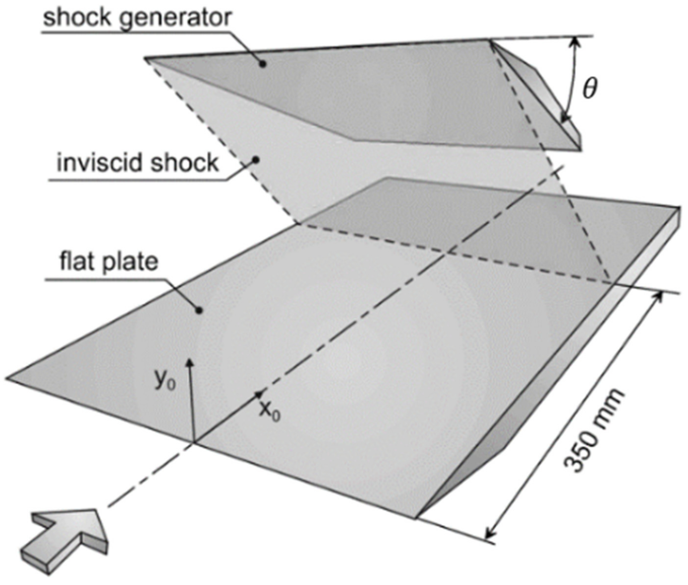
The numerical simulation in this study was conducted using an in-house code, which has been examined by plentiful studies and could acquire satisfying results in various flows, such as supersonic cavity flow and SWBLIs [25,30,34]. In the calculation process, the inviscid fluxes were discretized and reconstructed by Roe scheme with a second-order monotone upstream-centered schemes for conservation laws (MUSCL), and the central difference method was used for the discretization of viscous fluxes. The implicit lower-upper symmetric Gauss-Seidel (LUSGS) scheme was applied to time marching.

2.3.1. Flow Cases

This work focused on SWBLI in the form of a two-dimensional oblique shock wave impinging on the turbulent boundary layer and resulting in separation. The incident shock wave was generated by a shock generator whose configuration sketch is shown in Figure 1. This test model was derived from the SWBLI experimental studies conducted by Schulein et al. [6]. By adjusting the angle θ of the shock generator, the incident shock wave impinged on the flat plate with different angles and intensities, which caused various degrees of interaction. In Schulein’s experiments, θ was set to 6°, 10°, and 14°, which resulted in no separation, weak interaction with slight separation, and strong interference with large separation, respectively. In this work, the uncertainty analysis of the SST turbulence model’s parameters was carried out for the two cases with separation. The analysis results of the two cases could not only confirm each other on the whole, but also investigate the influence of the interaction degree on the parameters’ uncertainty analysis through the comparison of details. According to the experiment, the free-stream Mach number $M{a}_{\infty }$ was 5 and the Reynolds number $R{e}_{\infty }$ was $3.7\times {10}^7$(/m). The corresponding total pressure and total temperature were 2.12 MPa and 410 K. Additionally, the experimental data used for the comparison with numerical results in this study were all from Schulein et al. [8].

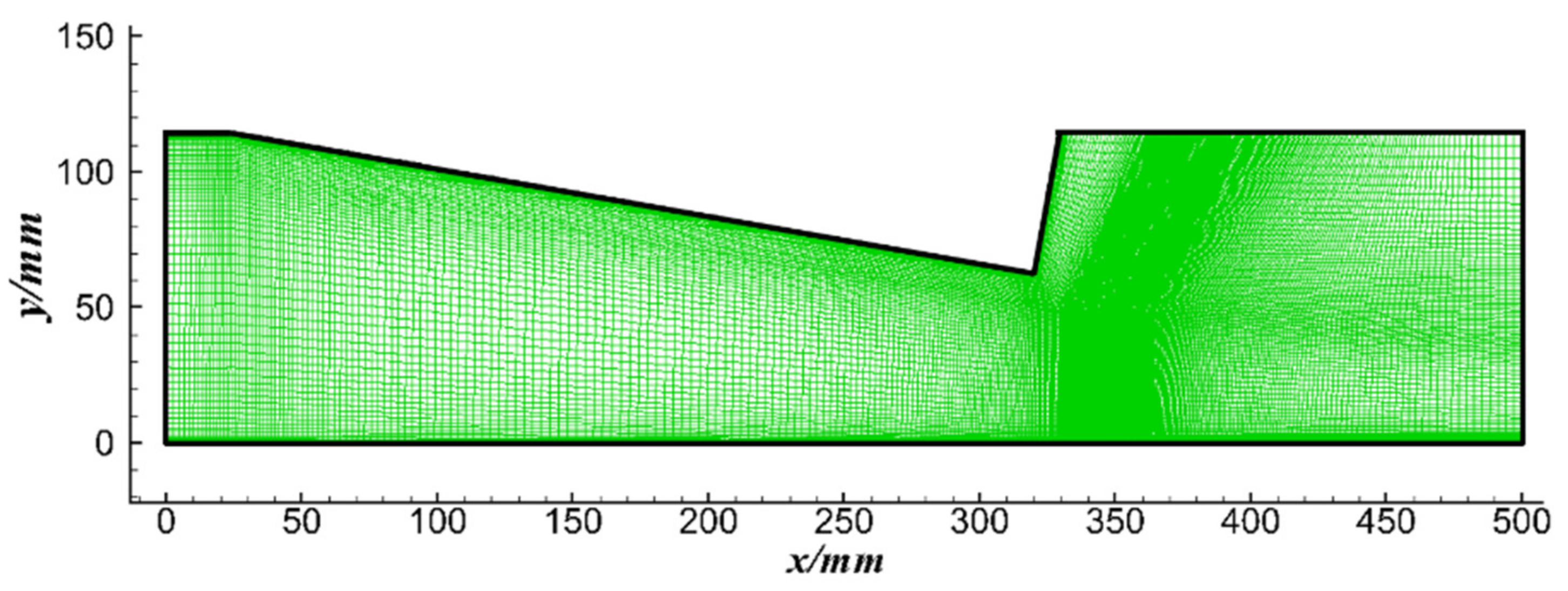
2.3.2. Grid Independence Analysis

Figure 2 presents the multi-block structured grid on the symmetry plane for the case with θ = 10°, refined in the interaction region. A non-slip isothermal condition was applied to both the upper and lower walls with $T_w=300K$ and periodic boundary conditions were imposed in the spanwise direction.

In order to ensure a sufficient resolution of the grid for simulation, grid independence analysis was performed via the grid convergence index (GCI) method [35], which has been evaluated over plentiful CFD cases and proved to be reliable for discretization error estimation. Three sets of grids with successively decreasing levels of grid resolutions $N_i\left(N_1=577\times 211\begin{array}{cc},& N_2=385\times 141\begin{array}{cc},& N_3=257\times 94\end{array}\end{array}\right)$ were tested, and ${\phi }_i$ represented the corresponding prediction results. In this method, the grid refinement factor $r_{i+1,i}$ is calculated as

$$r_{i+1,i}=\sqrt{N_i/N_{i+1}}.$$

(18)

And $p_{ob}$ represents the observed order of accuracy, expressed as

$$p_{ob}=\frac{1}{\ln (r_{21})}\left|\ln \left|{\epsilon }_{32}/{\epsilon }_{21}\right|+q(p_{ob})\right|\begin{array}{cc},& q(p_{ob})=\ln (\frac{r_{21}^{p_{ob}}-s}{r_{32}^{p_{ob}}-s})\end{array}\begin{array}{cc},& s=1\cdot \mathrm{sgn}(\frac{{\epsilon }_{32}}{{\epsilon }_{21}})\end{array},$$

(19)

where ${\epsilon }_{i+1,i}={\phi }_{i+1}-{\phi }_i$. The extrapolated value ${\phi }_{ext}^{21}$ is obtained via

$${\phi }_{ext}^{21}=\left(r_{21}^{p_{ob}}{\phi }_1-{\phi }_2\right)/\left(r_{21}^{p_{ob}}-1\right).$$

(20)

The approximate relative error $e_a^{i+1,i}$, extrapolated relative error $e_{ext}^{i+1,i}$, and the grid convergence index $GC{I}_{i+1,i}$ are calculated as

$$e_a^{i+1,i}=\left|\frac{{\phi }_{i+1}-{\phi }_i}{{\phi }_i}\right|\begin{array}{cc},& e_{ext}^{i+1,i}=\left|\frac{{\phi }_{ext}^{i+1,i}-{\phi }_i}{{\phi }_{ext}^{i+1,i}}\right|\end{array}\begin{array}{cc},& GC{I}_{i+1,i}=\frac{1.25e_a^{i+1,i}}{r_{i+1,i}^{p_{ob}}-1}\end{array}.$$

(21)

The wall pressure distributions of the three sets of grids for the θ = 10° are presented in Figure 3, as well as the extrapolated values and error bar calculated by GCI method. Overall, the calculation results of the SST turbulence model were in good agreement with the experimental values. The magnified view near the beginning of the separation in Figure 3a presents the difference in detail. The result of $N_3$ deviated more from the experimental data, while those of $N_1$ and $N_2$ were almost identical, which were closer to the extrapolated values and experimental data. The magnified view in Figure 3b indicates that with the occurrence of boundary layer separation, the discretization error increased gradually.

Table 2. The results of grid convergency calculations.

$\mathit{\phi }=\mathit{P}\left(\mathit{k}\mathit{P}\mathit{a}\right)$	${\mathit{N}}_1$	${\mathit{N}}_2$	${\mathit{N}}_3$	${\mathit{r}}_{21}$$, {\mathit{r}}_{32}$	${\mathit{\phi }}_1$	${\mathit{\phi }}_2$	${\mathit{\phi }}_3$
	577 × 211	385 × 141	257 × 94	1.5	5.410	5.254	4.918
	${\mathit{p}}_{\mathit{o}\mathit{b}}$	${\mathit{\phi }}_{\mathit{e}\mathit{x}\mathit{t}}^{\mathbf{21}}$	${\mathit{e}}_{\mathit{e}\mathit{x}\mathit{t}}^{\mathbf{21}}$	$\mathit{G}C{\mathit{I}}_{\mathbf{21}}$	${\mathit{e}}_{\mathit{e}\mathit{x}\mathit{t}}^{\mathbf{32}}$	$\mathit{G}\mathit{C}{\mathit{I}}_{\mathbf{32}}$
	1.89	5.545	2.43%	7.20%	11.30%	17.08%

displays the specific GCI analysis results of the wall pressure at x = 333.5 mm, where the $GC{I}_{21}$ was the maximum along the distribution. The $GC{I}_{21}<GC{I}_{32}$ indicated that the dependence of numerical results on grid scale was reduced. The maximum fine-gird convergence index was nearly 0.07. What’s more, except for the region near the separation point, the convergence indices were all below 0.01, suggesting the grid convergence has been achieved. Consequently, based on the above analysis, the grid with resolution $385\times 141$ was selected for subsequent studies.

3. Results and Discussion

In this section, the baseline results obtained by the SST turbulence model with the standard values assigned to parameters were discussed first to understand the flow structure and the predictive performance of the standard SST turbulence model in this flow’s simulation. Then, uncertainty quantification for the nine parameters in the SST turbulence model followed, quantitively assessing the effect of the parameters’ uncertainties on QoIs, which included wall pressure, skin friction, wall heat flux, and the positions of separation and reattachment points. Finally, sensitivity analysis was conducted to identify the key parameters contributing the most to the uncertainties generated in various QoIs.

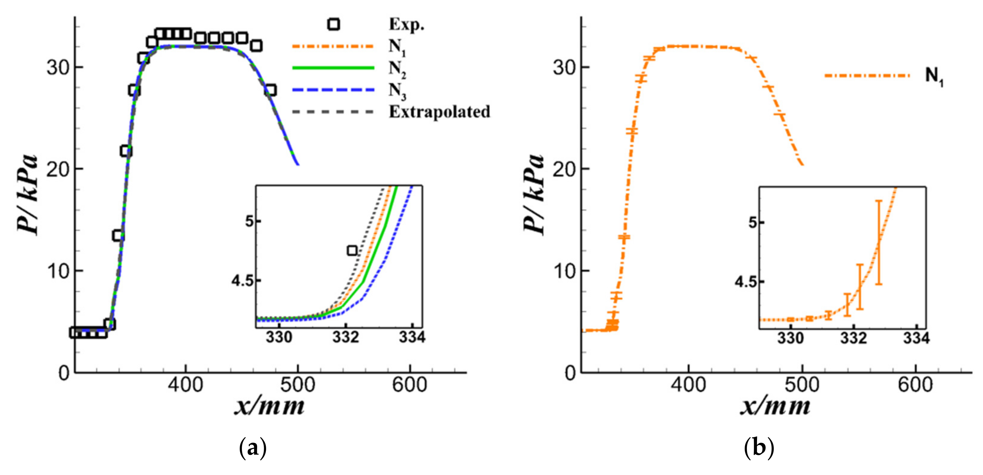
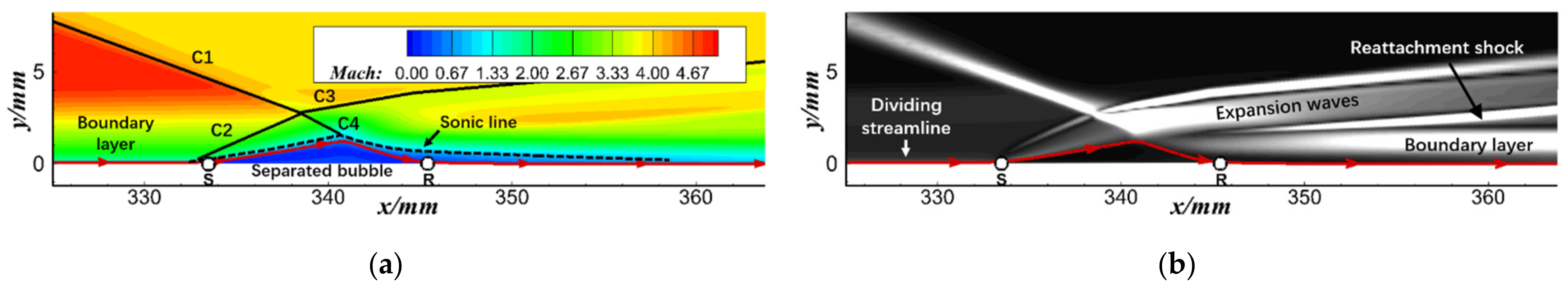
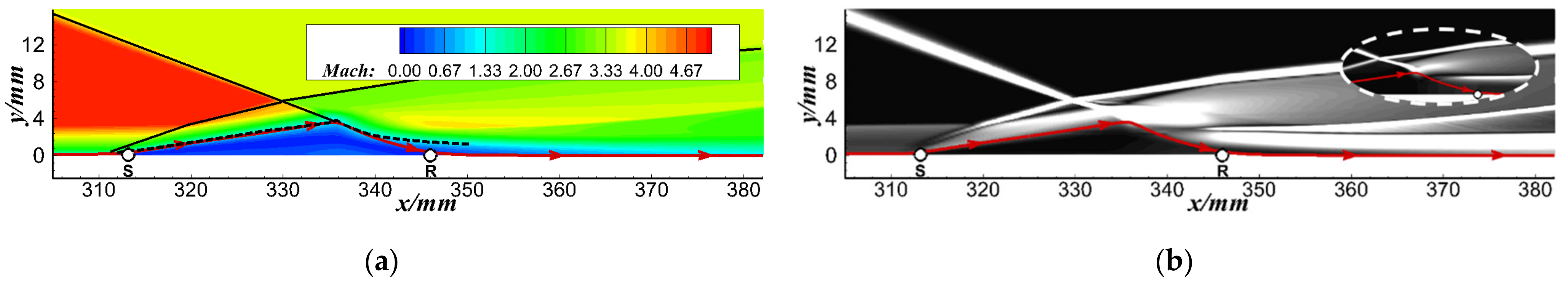
3.1. Baseline Results

Before uncertainty analysis, the SST turbulence model with standard parameters was used for simulating SWBLIs. Figure 4 and Figure 5 depict the flow structures of SWBLIs for the θ = 10° and θ = 14° cases, colored with Mach number and density gradient. Generally, the flow topological structures of the two cases resembled each other. Taking the result of the θ = 10° case as an example, the oblique incident shock wave C1 impinged the wall and caused the separation of the boundary layer. The separation shock wave C2 was generated as the boundary layer was lifted. Shock waves C1 and C2 intersected each other and then formed the refracted shock waves C3 and C4. After C4 being reflected by the separation bubble, an expansion fan was formed, which could be observed more distinctly in the magnified view with a pressure gradient contour in Figure 5b. Subsequently, the separated boundary layer began to reattach and formed a series of compression waves, which developed and converged into a reattachment shock wave. The separation and reattachment points were marked as S and R, respectively. In the θ = 10° case with weak interaction, the height of the separation bubble did not exceed the boundary layer thickness of the incoming flow. However, the size of the separation bubble enlarged when the interaction degree increased in the θ = 14° case, mainly reflected in the separation’s point moving forward and the increase in the separation bubble’s height.

The comparison of the positions of the separation and reattachment points, as well as the boundary layer thickness of incoming flow between the experiment and the computation, are tabulated in

Table 3. Comparison of the boundary layer thickness and the position of separation and reattachment between the experiment and simulation.

		Experiment	SST Turbulence Model
Boundary layer thickness at x = 296 mm		4.10 mm	4.08 mm
θ = 10°	Separation position	334.0 mm	333.5 mm
	Reattachment position	345.0 mm	345.4 mm
θ = 14°	Separation position	314.0 mm	313.2 mm
	Reattachment position	347.0 mm	345.7 mm

. There was little difference between the two cases, denoting that the SST model had a satisfactory performance in predicting the size of the separation region for SWBLIs.

Concerning the wall properties, the predicted distributions of wall pressure, skin friction, and wall heat flux are compared with experimental data for the two cases (as shown in Figure 6). The separation and reattachment points were marked as S and R with red arrows, respectively. The distributions of the wall properties rapidly increased after the boundary layer separation, which indicated the significant influence of the SWBLIs on high-speed vehicles’ dynamic and thermal loads. After reattachment, the wall properties continuously increased due to the compression waves, reaching a plateau or a peak at the place where the reattached boundary layer was most strongly compressed. Additionally, the last descending segment of the distributions resulted from the impact of the expansion wave generated at the trailing edge of the shock generator.

The comparison with the experimental data revealed the deficiencies of the SST turbulence model for predicting such flow. Although the model could accurately predict the locations of the separation and reattachment points, as well as the wall pressure distribution, it distinctively underestimated the skin friction and overestimated the wall heat flux after reattachment. These differences were further aggravated as the intensity of the interference increased. These defects were consistent with the evaluation of the SST turbulence model conducted by Brown [36], indicating that the SST turbulence model still required further improvement for predicting such flows with complex nonequilibrium characteristics (especially for heat transfer after reattachment).

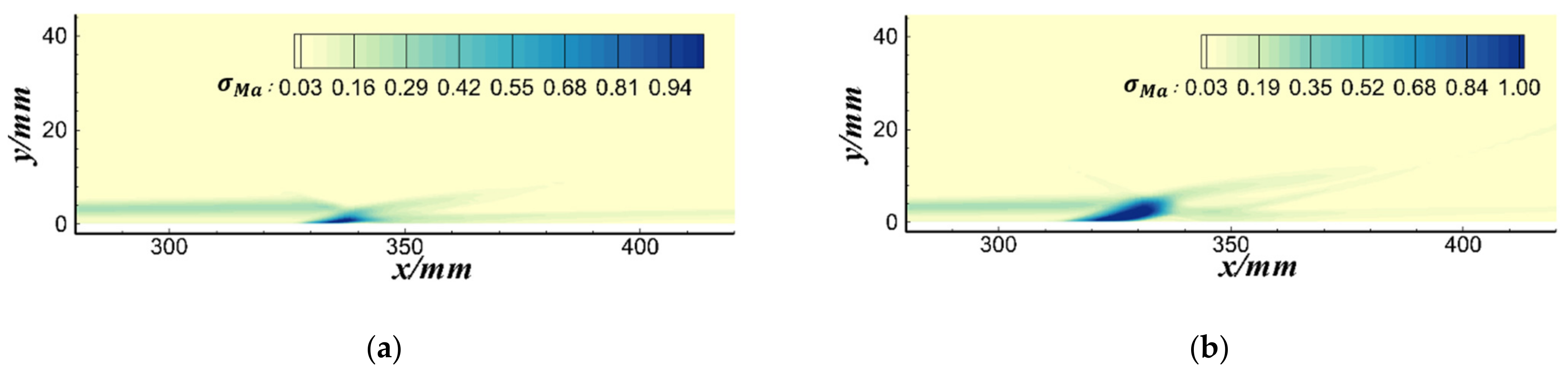
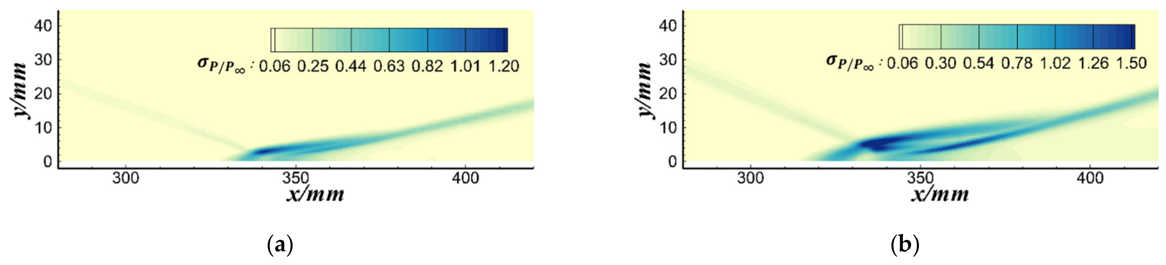
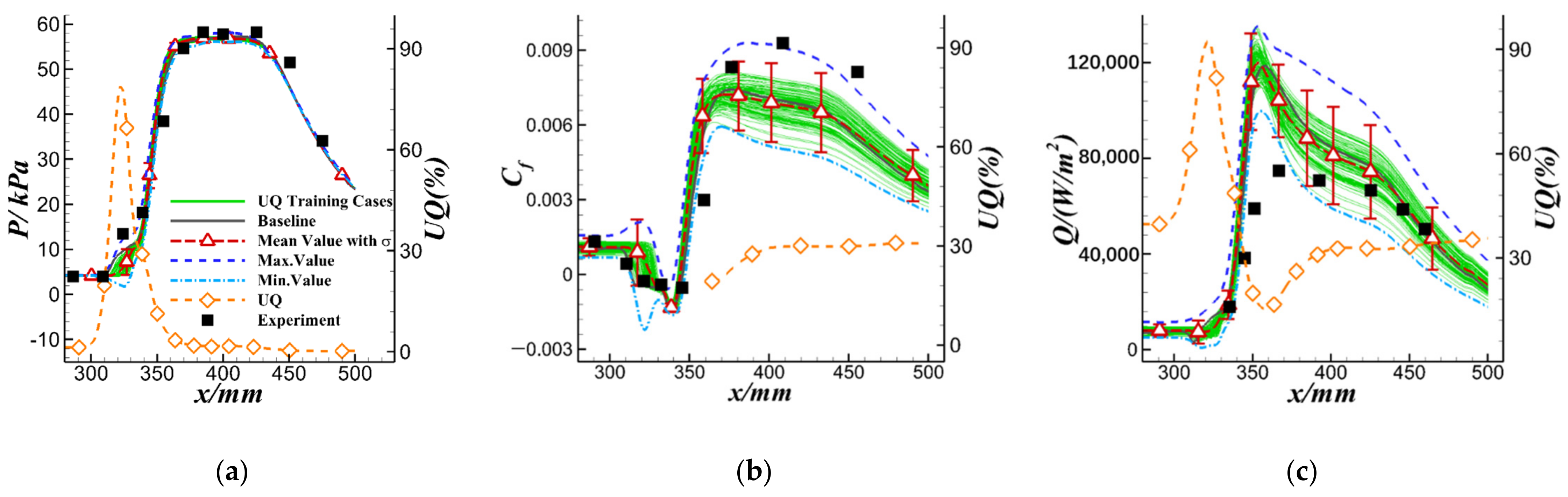
3.2. Uncertainty Quantification

In this section, the surrogate model was constructed by NIPC method to quantify the influence of the uncertainties in the model parameters on the results of QoIs by calculating the mean value, standard deviation, and uncertainty of QoIs. Figure 7 and Figure 8 display the standard deviation of Mach number and pressure coefficient contours on the two cases’ symmetry planes. For Mach number, the regions significantly affected by the uncertainty of the model parameters were the boundary layer of the incoming flow and the first half of the separation. Furthermore, except for the incident shock wave, the other shock waves influenced by the separation generated great uncertainties for the pressure coefficient.

In Figure 9 and Figure 10, the results of parameters’ uncertainty quantification for the wall pressure, skin friction and wall heat flux along the centerline of the plate in the two cases are displayed, including baseline results calculated using the standard SST turbulence model, results of 110 training cases calculated by the SST model with parameters assigned with sample values, and experimental data, as well as the mean value, standard deviation, and uncertainty boundaries $V_{max}$ and $V_{min}$ calculated by the surrogate model. The uncertainty of the model parameters slightly impacted the wall pressure, and the uncertainty generated in the wall pressure mainly concentrated in the separation zone. However, for the results of skin friction and wall heat flux, the uncertainty of the model parameters had a significant influence, especially at the plateau for skin friction, after the peak for wall heat flux and in the region of the separation for both. The distributions of quantified uncertainty (UQ) of the wall properties are also plotted in Figure 9 and Figure 10. One thing that needed to be explained here was the fact that since the skin friction was equal to zero at the positions of separation and reattachment points, the UQ could not be calculated. Therefore, the distributions of the UQ for skin friction were only presented after reattachment. Apparently, the prediction results in the separation region held the greatest uncertainty, which was mainly ascribed to different separation positions predicted in different training cases. For the region after reattachment, although the UQ here was not as great as that of separation, the higher pressure, skin friction, and heat flux, which would bring severe force and thermal loads to the aircraft in the field of engineering, made it also worth paying attention to.

Table 4. Uncertainty values of the wall properties and important positions.

	$\mathit{P}$	${\mathit{C}}_{\mathit{f}}$	$\mathit{Q}$	Separation Position	Reattachment Position	${\mathit{Q}}_{\mathit{m}\mathit{a}\mathit{x}}$	The Position of ${\mathit{Q}}_{\mathit{m}\mathit{a}\mathit{x}}$
θ = 10°	1.08%	23.24%	23.13%	2.4%	1.0%	11.64%	1.58%
θ = 14°	1.83%	29.52%	32.67%	3.32%	0.85%	17.55%	1.31%

lists the specific uncertainty values of QoIs, including P, $C_f$, and Q at x = 400 mm, the positions of separation and reattachment points, the peak of wall heat flux, and its position. As shown in the table, the uncertainty of the wall properties resulting from the uncertainty of model parameters approximated to 30%. Furthermore, with the increase in shock wave intensity, the influence of model parameters’ uncertainty was amplified, resulting in the increased uncertainty of wall properties and separation point location. However, the uncertainty of the positions of the reattachment point and heat flux peak slightly decreased, both of which were more deeply influenced by the incident shock wave.

The above analysis demonstrated that the uncertainty of the model parameters significantly influenced the prediction of SWBLIs. Therefore, when simulating such flows in engineering problems using the SST turbulence model, the influence of the model parameters’ uncertainty should be considered. It is necessary to provide uncertainty information on the basis of traditional determined results to increase the reliability of the numerical simulation. Meanwhile, the question concerning how to reduce the uncertainty of the turbulence model is also a challenge that requires further study.

3.3. Sensitivity Analysis

Further refining the contributions of the model parameters to the uncertainties generated in QoIs, the Sobol index for each parameter was calculated for the different QoIs to identify the key parameters that contributed the most to Qols’ uncertainties. By ranking the Sobol indices, the key parameters which had a profound influence on the prediction of QoIs could be identified. Each parameter’s Sobol index distribution for the wall pressure, skin friction, and wall heat flux in the two cases is provided in Figure 11 and Figure 12. For a clear display, the parameters with a quite small Sobol index were not shown. The bars colored with green, purple, and orange represented the uncertainty intervals of the positions of the separation point, the reattachment point and the peak of heat flux obtained in the uncertainty quantification analysis, respectively.

Generally, the Sobol index distributions of the model parameters in the two cases for the three wall properties were roughly consistent with each other. Obviously, the Sobol index of parameter ${\sigma }_{\omega 1}$ was the highest in the upstream and the far downstream of the separation region, where the turbulent boundary layer was not disturbed or gradually redeveloped, indicating that the prediction of the flow in these regions was greatly influenced by the uncertainty of parameter ${\sigma }_{\omega 1}$. This is due to the fact that in the area near the wall, the original k–ω model was predominant in the calculation, and the parameter with subscript 1 became critical for predictions. However, there was a strong adverse pressure gradient in the vicinity of the separation point and after reattachment, so that the Sobol index of parameter $a_1$ became the highest one almost throughout the separation region for the three wall properties. It is also worth noting that the Sobol index of parameter ${\beta }_1$ significantly increased at the peak of the wall heat flux, implying that the influence of ${\beta }_1$ on this QoI was significantly greater than the rest. From the perspective of the equations in the SST model, the parameter ${\beta }_1$ was involved in calculating the production term and dissipation term of the ω equation in the SST model, hence it had a greater influence on the dissipation of turbulent kinetic energy, and might further affect the prediction of the wall heat flux.

In the θ = 14° case, since the separation region was large enough, the influence of model parameter uncertainty on the prediction of the separation region could be observed more distinctly. Take the Sobol indices distribution for the wall pressure shown in Figure 12a as an example. The Sobol index of the parameter $a_1$ increased at the beginning of the separation, while then decreased near the center of the separation region due to the presence of the pressure platform where the Sobol index of parameter ${\sigma }_{\omega 1}$ dominated. However, with the reattachment of the boundary layer, the Sobol index of parameter ${\sigma }_{\omega 1}$ quickly decreased, while the Sobol index of parameter $a_1$ dominated gradually. Moreover, for the wall heat flux in Figure 12c, compared with the wall pressure, the distributions of Sobol indices in the separation zone were more complicated. Although parameter $a_1$ still dominated, its Sobol index fell to 0.6, while the Sobol indices for other parameters in the production and dissipation terms of the model increased to some extent. Besides that, the Sobol index of parameter ${\sigma }_{\omega 1}$ for the wall heat flux did not directly decrease to the bottom after separation as shown in Figure 12a but had a short rising stage during the descent.

Additionally, comparing Figure 11a and Figure 12a there was an noticeable difference in the latter half of the distribution, where the Sobol index of parameter $a_1$ suddenly increased as it approached x = 435 mm in the θ = 14° case, while maintaining a relative stability in the θ = 10° case. By observing the entire flow field, this difference could be attributed to the expansion wave at the trailing edge of the shock generator. As the angle of the shock generator changed, the position and angle of the expansion wave at the tail of the generator likewise changed, which further altered its influence on the boundary layer on the flat plate. As shown in Figure 6a, the initial position of the impact of expansion wave on the boundary layer was approximately x = 435 mm in the θ = 14° case, while for θ = 10°, this position was delayed to x = 450 mm, and the intensity of the expansion wave was relatively weak. However, Figure 9a and Figure 10a both indicated that the uncertainty of model parameters almost did not influence the wall pressure in this region. Thus, no further analysis was required.

With respect to the position of the separation and reattachment points, the bar graphs of the Sobol indices of the parameters are illustrated in Figure 13. Apparently, the parameter $a_1$ was the most significant factor affecting the prediction of the separation point among the nine parameters. Additionally, for the reattachment point, the Sobol index of parameter $a_1$ decreased but still played a leading role, followed by parameter ${\sigma }_{\omega 1}$.

Thus, the model parameters $a_1$ and ${\sigma }_{\omega 1}$ were the main contributors to the uncertainties in QoIs. Besides that, the parameter ${\beta }_1$ had the greatest influence on the uncertainty of the wall heat flux peak. Among the remaining parameters, $\kappa$ and ${\beta }^{*}$ also contributed to the uncertainty of the wall properties in the region of the attached boundary layer. Altogether, the identification of key parameters provided guidelines for the subsequent correction of the model and its practical applications.

Finally, a more detailed analysis of the identified key parameters $a_1$, ${\sigma }_{\omega 1}$, and ${\beta }_1$ was carried out. By separately changing these parameters to the boundary value of their uncertainty intervals in the θ = 10° case, the influences of these parameters on the prediction results were analyzed.

The comparison of the dimensionless turbulent eddy viscosity contours for seven test cases is presented in Figure 14, including the baseline results with standard model parameters and the results with the changed parameters. Figure 15 displays the skin friction and wall heat flux distributions for these cases. As uncertainty quantification analysis has demonstrated that the wall pressure was not sensitive to the uncertainties in the model parameters, the result of this QoI was not shown here. In Figure 14, increasing parameters $a_1$ and ${\sigma }_{\omega 1}$ could lead to a growth in the eddy viscosity of the incoming boundary layer, and this effect was amplified by the SWBLI, dramatically enlarging the eddy viscosity in the boundary layer after reattachment, which resulted in a significant increase in the skin friction and wall heat flux after the peak (as shown in Figure 15). However, the difference between the two cases was that increasing $a_1$ significantly delayed the location of the separation point and caused the separation area to almost disappear. The increase of ${\sigma }_{\omega 1}$ could only slightly delay the separation point. This difference might be related to the blending functions $F_1$ and $F_2$, limiting the scope of the influence of the two parameters. Based on the turbulent eddy viscosity calculation formula in the SST model, parameter $a_1$ was involved only in the simulation in the region with a high strain rate, limited by blending function $F_2$ simultaneously. The boundary layer in the vicinity of the separation point held a strong strain rate, so changing the value of parameter $a_1$ could affect the separation point position. However, for the parameter ${\sigma }_{\omega 1}$ limited by the blending function $F_1$, Figure 16 illustrates that $F_1$ rapidly decreased at the starting position of the separation, thus the change in parameter ${\sigma }_{\omega 1}$ was unable to generate the same effect on the prediction of the separation point as $a_1$.

As for ${\beta }_1$, its influence on the prediction of eddy viscosity (dimensionless) was not as apparent as that of the first two parameters shown in Figure 14. According to the distributions of skin friction and wall heat flux plotted in Figure 15, the influence of parameter ${\beta }_1$ on the flow was mainly concentrated in the vicinity of the separation zone. The decrease in ${\beta }_1$ brought about the delay of the separation, and the descending peak value of the wall heat flux after reattachment.

Through the above analysis, we further understood how key model parameters affected the prediction of such flow and further deepened our cognition of these model parameters.

4. Conclusions

In the current study, detailed research on uncertainty analysis of the SST turbulence model’s parameters was carried out for SWBLIs in the form of an oblique shock wave impinging on the turbulent boundary layer and inducing separation. Firstly, a surrogate model between the model parameters and the simulation results was constructed using the NIPC method to quantify the influence of the parameters’ uncertainties on the QoIs. In the subsequent sensitivity analysis, based on the variances calculated by the constructed surrogate model, the Sobol index of each model parameter for the different QoIs was acquired, and the key parameters were identified. Furthermore, the specific influence of the key parameters on the simulation results of SWBLIs was analyzed. The conclusions are as follows:

• The flow mechanism of SWBLIs was highly intricate. Although the SST turbulence model could simulate the basic interaction process and accurately predict the position of the separation point, there were obvious deviations between the prediction results and the experimental data for the skin friction and wall heat flux after reattachment.
• The uncertainty of the model parameters had a significant influence on the prediction results. For the spatial flow field, the uncertainty of the model parameters generated significant uncertainty in the prediction of the Mach number in the separation region and the prediction of pressure at the shock waves caused by separation. For those wall properties, although the parameters’ uncertainties had little effect on the prediction of the wall pressure, the uncertainties of the skin friction and wall heat flux in the boundary layer after reattachment were nearly 30%. Moreover, the influence of the parameters’ uncertainty was intensified with an increase in incident shock wave intensity for most of QoIs. Therefore, the parameters’ uncertainties should be considered in engineering to increase the reliability and completeness of the RANS results.
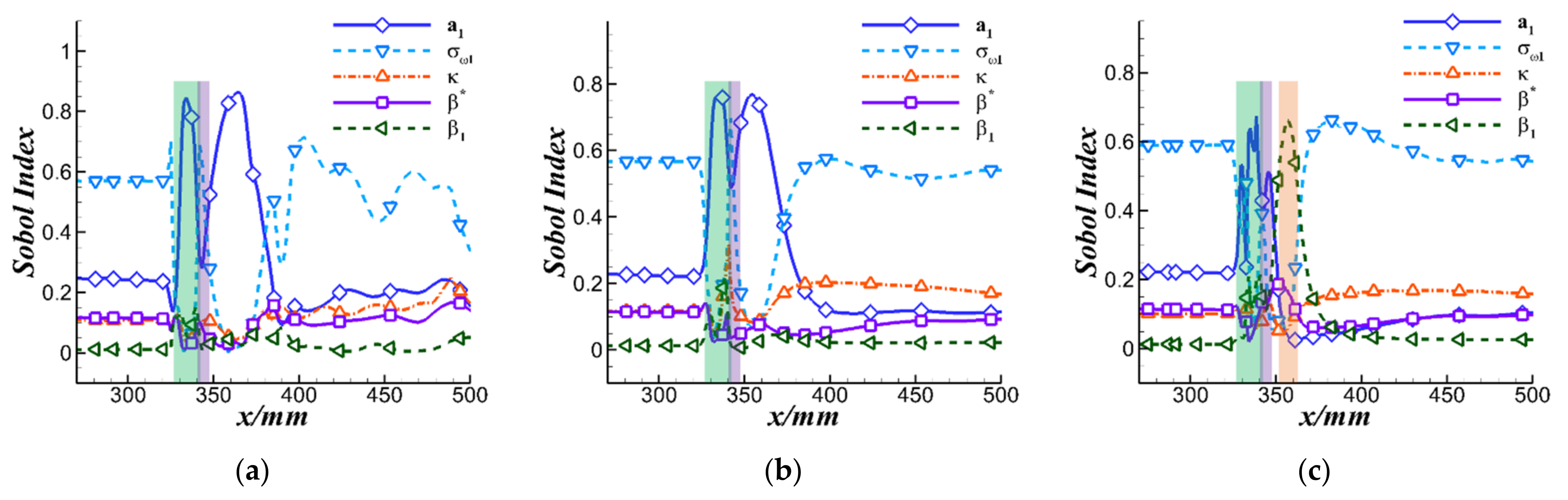
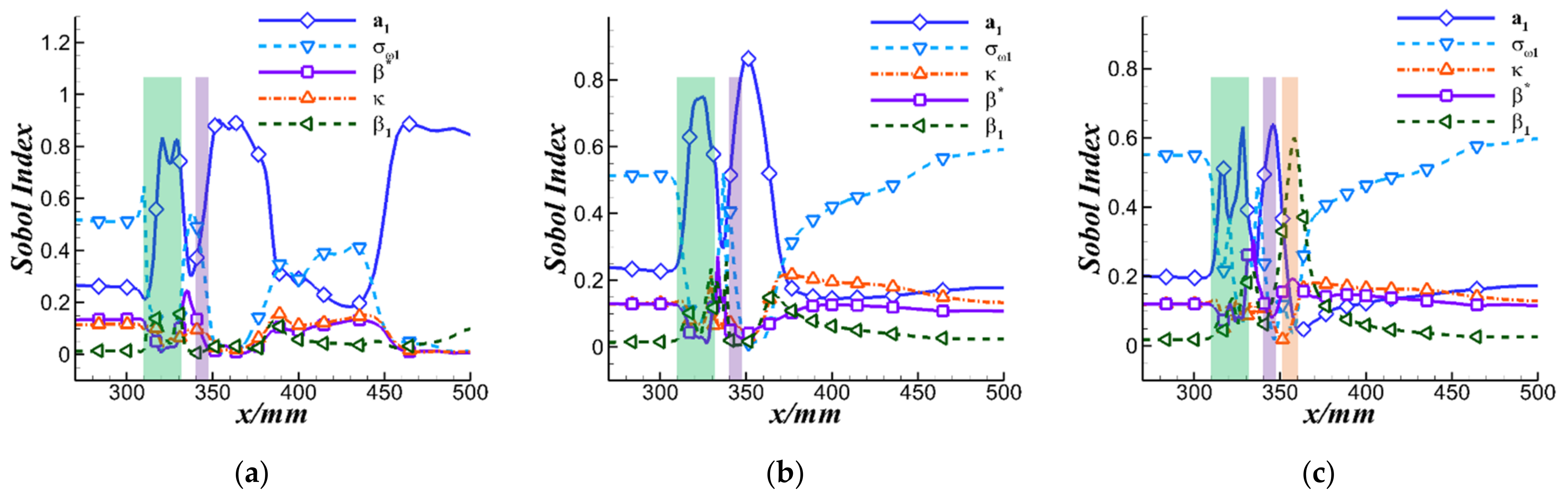
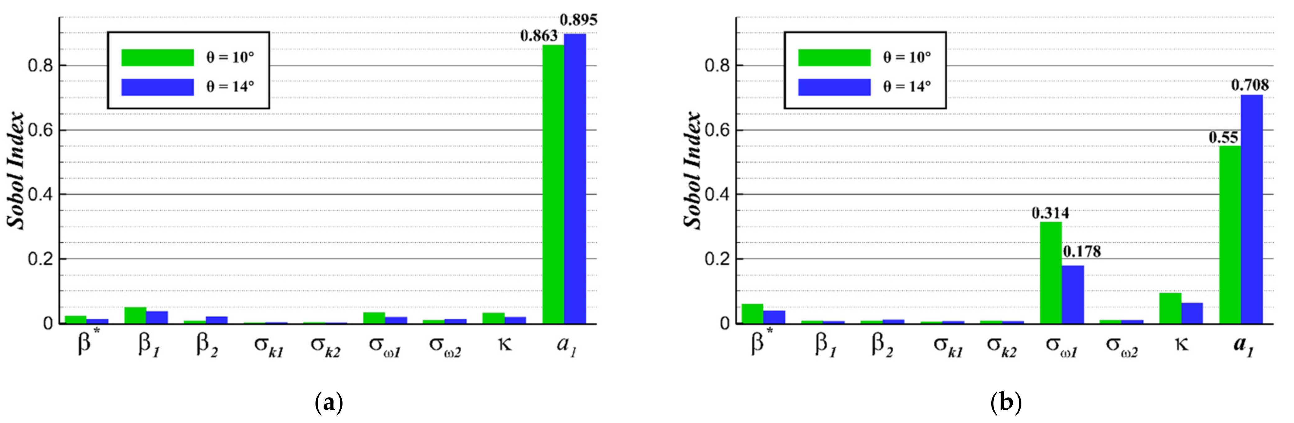
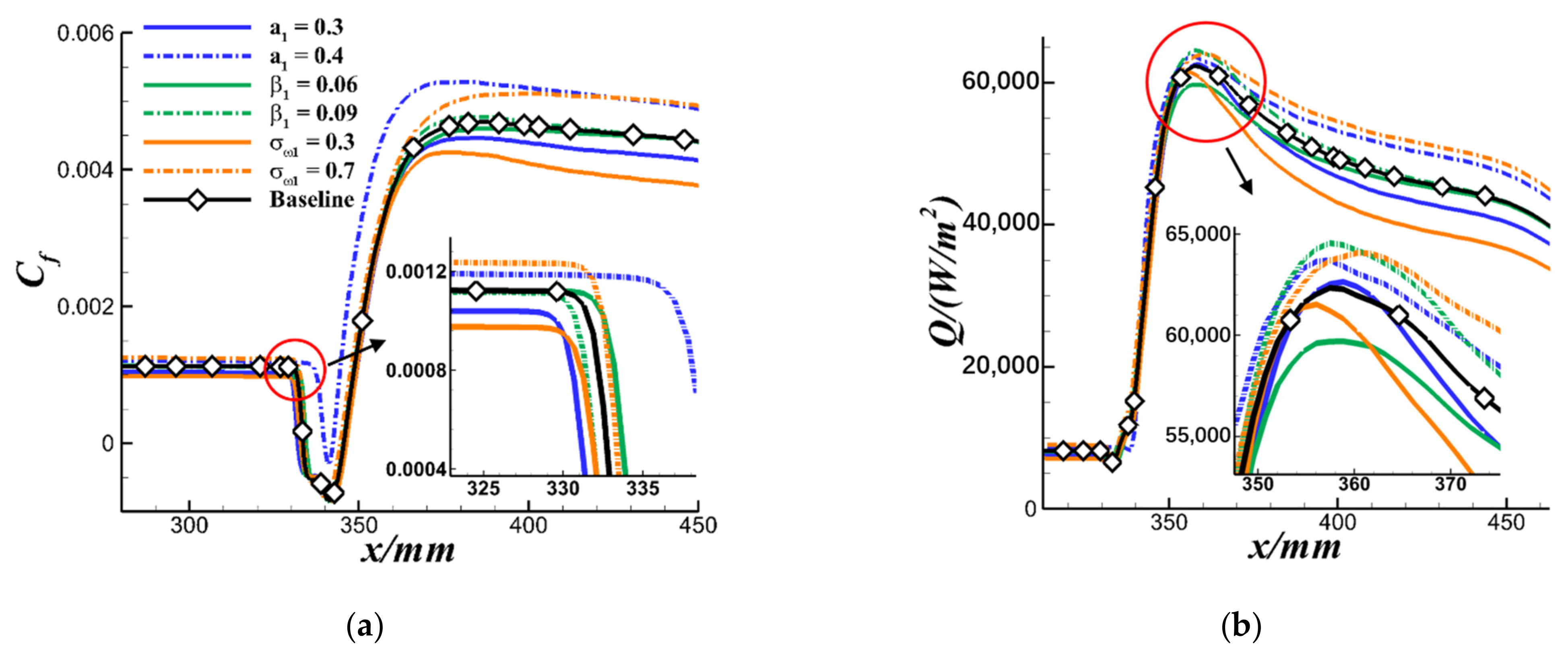
• Through sensitivity analysis, based on the results of the parameters’ Sobol index for different QoIs, the key parameters that contributed most to the uncertainties generated in QoIs were $a_1$, ${\sigma }_{\omega 1}$, and ${\beta }_1$. Furthermore, by changing those model parameters separately, their effects on the prediction of the average flow were investigated. Among them, parameter $a_1$ had the most crucial influence on the prediction of the separation point; parameter ${\sigma }_{\omega 1}$ mainly influenced the skin friction and wall heat flux after reattachment; and parameter ${\beta }_1$ was responsible for the uncertainties in the peak of heat flux. The identification and further study of key parameters can deepen the cognition of the model parameters and provide a reference for engineering applications as well as potential guidance for the model’s future improvement.

References

1. Chung, K.-M.; Huang, Y.-X. Global Visualization of Compressible Swept Convex-Corner Flow Using Pressure-Sensitive Paint. Aerospace 2021, 8, 106. [Google Scholar] [CrossRef]
2. Chung, K.-M.; Su, K.-C.; Chang, K.-C. The Effect of Vortex Generators on Shock-Induced Boundary Layer Separation in a Transonic Convex-Corner Flow. Aerospace 2021, 8, 157. [Google Scholar] [CrossRef]
3. Semlitsch, B.; Mihăescu, M. Fluidic Injection Scenarios for Shock Pattern Manipulation in Exhausts. AIAA J. 2018, 56, 4640–4644. [Google Scholar] [CrossRef]
4. Semlitsch, B.; Mihăescu, M. Evaluation of Injection Strategies in Supersonic Nozzle Flow. Aerospace 2021, 8, 369. [Google Scholar] [CrossRef]
5. Running, C.L.; Juliano, T.J. Global Skewness and Coherence for Hypersonic Shock-Wave/Boundary-Layer Interactions with Pressure-Sensitive Paint. Aerospace 2021, 8, 123. [Google Scholar] [CrossRef]
6. Schülein, E.; Krogmann, P.; Stanewsky, E. Documentation of Two-Dimensional Impinging Shock/Turbulent Boundary Layer interaction Flow; Institute of Aerodynamics and Flow Technology: Göttingen, Germany, 1996; pp. 1–65. [Google Scholar]
7. Fedorova, N.N.; Fedorchenko, I.A.; Schülein, E. Experimental and Numerical Investigation of the Oblique Shock Wave/Turbulent Boundary Layer Interaction at M=5. J. Appl. Math. Mech. 2001, 81, 773–774. [Google Scholar] [CrossRef]
8. Schülein, E. Skin Friction and Heat Flux Measurements in Shock/Boundary Layer Interaction Flows. AIAA J. 2006, 44, 1732–1741. [Google Scholar] [CrossRef]
9. Duraisamy, K.; Spalart, P.R.; Rumsey, C.L. Status, Emerging Ideas and Future Directions of Turbulence Modeling Research in Aeronautics; Technical Memorandum NASA/TM–2017–219682; NASA: Hampton, VA, USA, 2017. [Google Scholar]
10. Thivet, F.; Knight, D.D.; Zheltovodov, A.A.; Maksimov, A.I. Insights in Turbulence Modeling for Crossing-Shock-Wave/Boundary-Layer Interactions. AIAA J. 2001, 39, 985–995. [Google Scholar] [CrossRef]
11. Steelant, J. Effect of a compressibility correction on different turbulence models. Eng. Turbul. Modell. Exp. 2002, 5, 207–216. [Google Scholar]
12. Morkovin, M.V. Effects of Compressibility on Turbulent Flows; de la Turbulence, M., Favre, A., Eds.; Gordon and Breach: New York, NY, USA, 1964. [Google Scholar]
13. Xiao, X.; Hassan, H.A.; Edwards, J.R.; Gaffney, R.L. Role of Turbulent Prandtl Numbers on Heat Flux at Hypersonic Mach Numbers. AIAA J. 2007, 45, 806–813. [Google Scholar] [CrossRef]
14. Roy, S.; Pathak, U.; Sinha, K. Variable Turbulent Prandtl Number Model for Shock/Boundary-Layer Interaction. AIAA J. 2018, 56, 342–355. [Google Scholar] [CrossRef]
15. Lillard, R.P.; Oliver, B.; Olsen, M.; Blaisdell, G.; Lyrintzis, A. The lagRST Model: A Turbulence Model for Non-Equilibrium Flows. In Proceedings of the 50th AIAA Aerospace Sciences Meeting including the New Horizons Forum and Aerospace Exposition, Nashville, TN, USA, 9–12 January 2012. [Google Scholar]
16. Slotnick, J.; Khodadoust, A.; Alonso, J.; Darmofal, D.; Gropp, W.; Lurie, E.; Mavriplis, D. CFD Vision 2030 Study: A Path to Revolutionary Computational Aerosciences; Technical Publication NASA/CR-2014-218178; NASA: Hampton, VA, USA, 2014. [Google Scholar]
17. Durbin, P.A. Some Recent Developments in Turbulence Closure Modeling. Annu. Rev. Fluid Mech. 2018, 50, 77–103. [Google Scholar] [CrossRef]
18. Xiao, H.; Cinnella, P. Quantification of model uncertainty in RANS simulations: A review. Prog. Aerosp. Sci. 2019, 108, 1–31. [Google Scholar] [CrossRef] [Green Version]
19. Menter, F.R. Two-equation eddy-viscosity turbulence models for engineering applications. AIAA J. 1994, 32, 1598–1605. [Google Scholar] [CrossRef] [Green Version]
20. Matyushenko, A.A.; Garbaruk, A.V. Adjustment of the k-ω SST turbulence model for prediction of airfoil characteristics near stall. In Proceedings of the 18th International Conference PhysicA.SPb , Saint-Petersburg, Russia, 26–29 October 2015. [Google Scholar]
21. Hu, Y. Research on the Effects of Numerical Simulation Parameters of Separation Vortex Flow Field. J. Mech. Eng. 2016, 52, 165–172. [Google Scholar] [CrossRef]
22. Schaefer, J.; Hosder, S.; West, T.; Rumsey, C.; Carlson, J.-R.; Kleb, W. Uncertainty Quantification of Turbulence Model Closure Coefficients for Transonic Wall-Bounded Flows. AIAA J. 2017, 55, 195–213. [Google Scholar] [CrossRef]
23. Erb, A.J.; Hosder, S. Uncertainty Analysis of Turbulence Model Closure Coefficients for Shock Wave-Boundary Layer Interaction Simulations. In Proceedings of the 2018 AIAA Aerospace Sciences Meeting, Kissimmee, FL, USA, 8–12 January 2018. [Google Scholar]
24. Di Stefano, M.A.; Hosder, S.; Baurle, R.A. Effect of Turbulence Model Uncertainty on Scramjet Isolator Flowfield Analysis. J. Propul. Power 2020, 36, 109–122. [Google Scholar] [CrossRef]
25. Zhao, Y.; Yan, C.; Wang, X.; Liu, H.; Zhang, W. Uncertainty and sensitivity analysis of SST turbulence model on hypersonic flow heat transfer. Int. J. Heat Mass Transfer. 2019, 136, 808–820. [Google Scholar] [CrossRef]
26. Subbian, G.; Botelho e Souza, A.C.; Radespiel, R.; Zander, E.; Friedman, N.; Moshagen, T.; Moioli, M.; Breitsamter, C.; Sørensen, K.A. Calibration of an extended Eddy Viscosity Turbulence Model using Uncertainty Quantification. In Proceedings of the AIAA Scitech 2020 Forum, Orlando, FL, USA, 6–10 January 2020. [Google Scholar]
27. Li, J.; Chen, S.; Cai, F.; Wang, S.; Yan, C. Bayesian uncertainty analysis of SA turbulence model for supersonic jet interaction simulations. Chin. J. Aeronaut. 2021, 35, 185–201. [Google Scholar] [CrossRef]
28. Han, D.; Hosder, S. Inherent and Model-Form Uncertainty Analysis for CFD Simulation of Synthetic Jet Actuators. In Proceedings of the 50th AIAA Aerospace Sciences Meeting including the New Horizons Forum and Aerospace Exposition, Nashville, TN, USA, 9–12 January 2012. [Google Scholar]
29. Eldred, M.; Webster, C.; Constantine, P. Evaluation of Non-Intrusive Approaches for Wiener-Askey Generalized Polynomial Chaos. In Proceedings of the 49th AIAA/ASME/ASCE/AHS/ASC Structures, Structural Dynamics, and Materials Conference, Schaumburg, IL, USA, 7–10 April 2008. [Google Scholar]
30. Liu, H.; Yan, C.; Zhao, Y.; Qin, Y. Uncertainty and sensitivity analysis of flow parameters on aerodynamics of a hypersonic inlet. Acta Astronaut. 2018, 151, 703–716. [Google Scholar] [CrossRef]
31. McKay, M.D.; Beckman, R.J.; Conover, W.J. Comparison of Three Methods for Selecting Values of Input Variables in the Analysis of Output from a Computer Code. Technometrics 1979, 21, 239–245. [Google Scholar]
32. Hosder, S.; Walters, R.; Balch, M. Efficient Sampling for Non-Intrusive Polynomial Chaos Applications with Multiple Uncertain Input Variables. In Proceedings of the 48th AIAA/ASME/ASCE/AHS/ASC Structures, Structural Dynamics, and Materials Conference, Honolulu, HI, USA, 23–26 April 2007. [Google Scholar]
33. Crestaux, T.; Le Maıtre, O.; Martinez, J.-M. Polynomial chaos expansion for sensitivity analysis. Reliab. Eng. Syst. Saf. 2009, 94, 1161–1172. [Google Scholar] [CrossRef]
34. Zhou, L.; Zhao, R.; Yuan, W. An investigation of interface conditions inherent in detached-eddy simulation methods. Aerosp. Sci. Technol. 2018, 74, 46–55. [Google Scholar] [CrossRef]
35. Celik, I.B.; Ghia, U.; Roache, P.J.; Freitas, C.J.; Coleman, H.; Raad, P.E. Procedure for Estimation and Reporting of Uncertainty Due to Discretization in CFD Applications. J. Fluids Eng. 2008, 130, 07800101–07800104. [Google Scholar]
36. Brown, J.L. Shock Wave Impingement on Boundary Layers at Hypersonic Speeds: Computational Analysis and Uncertainty. In Proceedings of the 42nd AIAA Thermophysics Conference, Honolulu, HI, USA, 27–30 June 2011. [Google Scholar]
Figure 1. Sketch of the shock generator.
Aerospace 09 00055 g001
Figure 2. Grid on the symmetry plane.
Aerospace 09 00055 g002
Figure 3. (a) Wall pressure distributions along the center line on the flat plate; (b) N 1 solution, with discretization error bar G C I 21 .
Aerospace 09 00055 g003
Figure 4. Flow structure on the symmetry plane for θ = 10° case. (a) Mach number contour; (b) density gradient contour.
Aerospace 09 00055 g004
Figure 5. Flow structure on the symmetry plane for θ = 14° case. (a) Mach number contour; (b) density gradient contour.
Aerospace 09 00055 g005
Figure 6. Comparison of the wall properties distribution between the experiment and simulation for the two cases. (a) Wall pressure; (b) skin friction; (c) wall heat flux.
Aerospace 09 00055 g006
Figure 7. Standard deviation of Mach number contour for the two cases. (a) θ = 10°; (b) θ = 14°.
Aerospace 09 00055 g007
Figure 8. Standard deviation of pressure coefficient contour for the two cases. (a) θ = 10°; (b) θ = 14°.
Aerospace 09 00055 g008
Figure 9. Distribution of the wall properties with uncertainty analysis results for θ = 10° case. (a) Wall pressure; (b) skin friction; (c) wall heat flux.
Aerospace 09 00055 g009
Figure 10. Distributions of the wall properties with uncertainty analysis results for θ = 14° case. (a) Wall pressure; (b) skin friction; (c) wall heat flux.
Aerospace 09 00055 g010
Figure 11. Distributions of the Sobol indices of model’s parameters for the wall properties in θ = 10° case. (a) Wall pressure; (b) skin friction; (c) wall heat flux.
Aerospace 09 00055 g011
Figure 12. Distributions of the Sobol indices of model’s parameters for the wall properties in θ = 14° case. (a) Wall pressure; (b) skin friction; (c) wall heat flux.
Aerospace 09 00055 g012
Figure 13. Sobol indices of model’s parameters for the separation and reattachment positions in two cases. (a) Position of the separation point; (b) position of the reattachment point.
Aerospace 09 00055 g013
Figure 14. Eddy viscosity contour for test cases.
Aerospace 09 00055 g014
Figure 15. Distribution of the wall properties on the plate for test cases. (a) Skin friction; (b) wall heat flux.
Aerospace 09 00055 g015
Figure 16. F 1 contour of the results in the standard SST model.
Aerospace 09 00055 g016