1. Introduction
Microturbines are scaled-down turboshafts or turbojets with rotating components similar to those used in piston engine turbochargers [
1,
2]. They have a single- or double-stage radial compressor and a radial or axial turbine. The rotational speed is usually greater than 70,000 revolutions per minute, and for some applications it exceeds 200,000 rpm.
Microturbines have many promising applications. One major use is energy generation [
3,
4], primarily as standby or backup power, where power availability is critical. Testing alternative fuels is another area where microturbines are widely used: in fact, they make it possible to evaluate jet fuels synthesised in small quantities [
5,
6]. The use of propelling Unmanned Aerial Vehicles (UAV) or Light Personal Aircraft has been increasing over the last years [
7,
8,
9], as more producers offer many types of micro and small turbojets or turboprops in a wide range of classes [
10,
11]. However, engine downsizing is accompanied by a significant increase in Reynolds number, resulting in a decrease in overall engine performance [
12]. Because of this, research to understand the behaviour and performance of microturbines [
13,
14] is critical, specifically by implementing simulation models. They can be used, among others, to improve engine performance by converting micro turbojets to turbofans [
15,
16] or optimizing their exhaust nozzle [
17,
18].
Modelling the dynamics of a complex non-linear system, such as a gas turbine, makes it possible to control it effectively and monitor its performance [
19]. Traditional engine models rely on the thermodynamic description of the engine, so they are called white-box or model-based approaches. Transient simulation requires representation of the changes of gas density in plenum volumes using the inter-component volume method [
20,
21,
22]. Alternatively, the constant mass flow (CMF) iterative method can be used in dynamic simulations [
23,
24,
25]. Chachurski et al. [
26] developed a steady-state mathematical model of the JETPOL GTM 120 micro turbojet and validated it with test rig data. Several advanced models of JetCat engines were presented [
27,
28,
29]. However, many published models of microturbines, for example, [
30,
31,
32] do not use component maps. Such models are valid only for design-point or steady-state operation due to considerable simplifications in their structure. Engine control systems are also usually based on linearized models due to the required low response times [
33,
34,
35].
A reliable transient model is necessary to simulate a gas-turbine engine propelling a highly maneuverable aircraft. Such a model needs component maps [
19,
36] to describe how the engine performs at nearly any design or off-design conditions. In practice, component maps for turbomachinery are generated in three different ways: by component rig testing, aerodynamic analysis, or scaling existing maps. For microturbines, component maps are primarily generated with CFD tools, for example, for radial compressors [
28,
37,
38], turbines [
39] and combustors [
40,
41]. What is more, a complete CFD model of the gas path was developed recently, which simulates engine performance without component maps [
42].
Accurate maps are rarely available, so different map scaling and adaptation methods are commonly used [
43,
44,
45]. The first-choice method is single point scaling [
46] because it is built into GSP and other tools. However, it works properly only for components with similar geometry that is proportionally scaled up or down. Applying factors and deltas [
19] is a linear method for three-dimensional map transformation. Such map operations should preserve the physical sense of the flow, in particular its Mach number [
36]. Otherwise, scaled maps are valid only in the vicinity of experimental points they are based on.
During their operational life engine components are subject to several physical problems such as fouling, erosion, corrosion, blade damage, tip clearance increase, worn seals, combustor damage, and many others. The performance degradation of the engine depends on the type and severity of the deterioration and the components that are deteriorated. Generally, a deteriorated gas turbine provides less power for a certain amount of fuel mass flow or needs more fuel to produce a certain amount of power [
19,
47]. The severity of component deterioration can be characterized by the difference between the actual component condition parameters and their baseline. From a thermodynamic perspective the condition of gas path components is quantified in terms of isentropic efficiency
, mass flow W and pressure ratio PR.
Model-based gas path analysis systems make it possible to monitor engine performance parameters for fault diagnosis and manage component deterioration [
48,
49]. However, data-driven approaches are more and more common recently, not only in full-scale engines but also in microturbines [
50,
51]. Often, engine parameters are estimated or predicted by machine learning techniques which are trained with data obtained from simplified aeroengine gas-path performance prognostic models. For example, a transient model of the Viper 632-43 turbojet was implemented in our earlier project [
52]. An integrated health monitoring platform for performance analysis and degradation diagnostics of gas turbine engines was demonstrated [
47,
53]. These studies underlined the suitability of Gas Path Analysis tools to predict aeroengine performance with a high accuracy. However, few works deal with the implementation of such models for small scale aeroengines.
To sum up, most publications on microturbine simulation are based on simplified models which hardly describe transient operation. Some micro turbojets were tested in a wind tunnel to study their performance in low-altitude flight [
31,
54]. Although several transient models of microturbines [
20,
55,
56] were developed, they usually lacked validation with real flight data.
The purpose of this work was to create a numerical model of a microturbine under transient conditions, validated with experimental flight data. The model is intended for predicting emissions and generating training datasets for an artificial neural network (ANN), for the purpose of a planned engine health management system. There were three crucial tasks to develop the model:
Use of test-rig data from two micro-turbines with the same thrust and size to define their operating points and create compressor and turbine maps. A least-squares scaling method was employed to transform the maps using parameters from four different engine operating points;
Development and fine-tuning of the numerical model in GSP (Gas turbine Simulation Program) [
57,
58]: The model was used for simulation of the design point, steady states at various engine speeds, and also flight missions to model the behaviour of the engine under transient conditions;
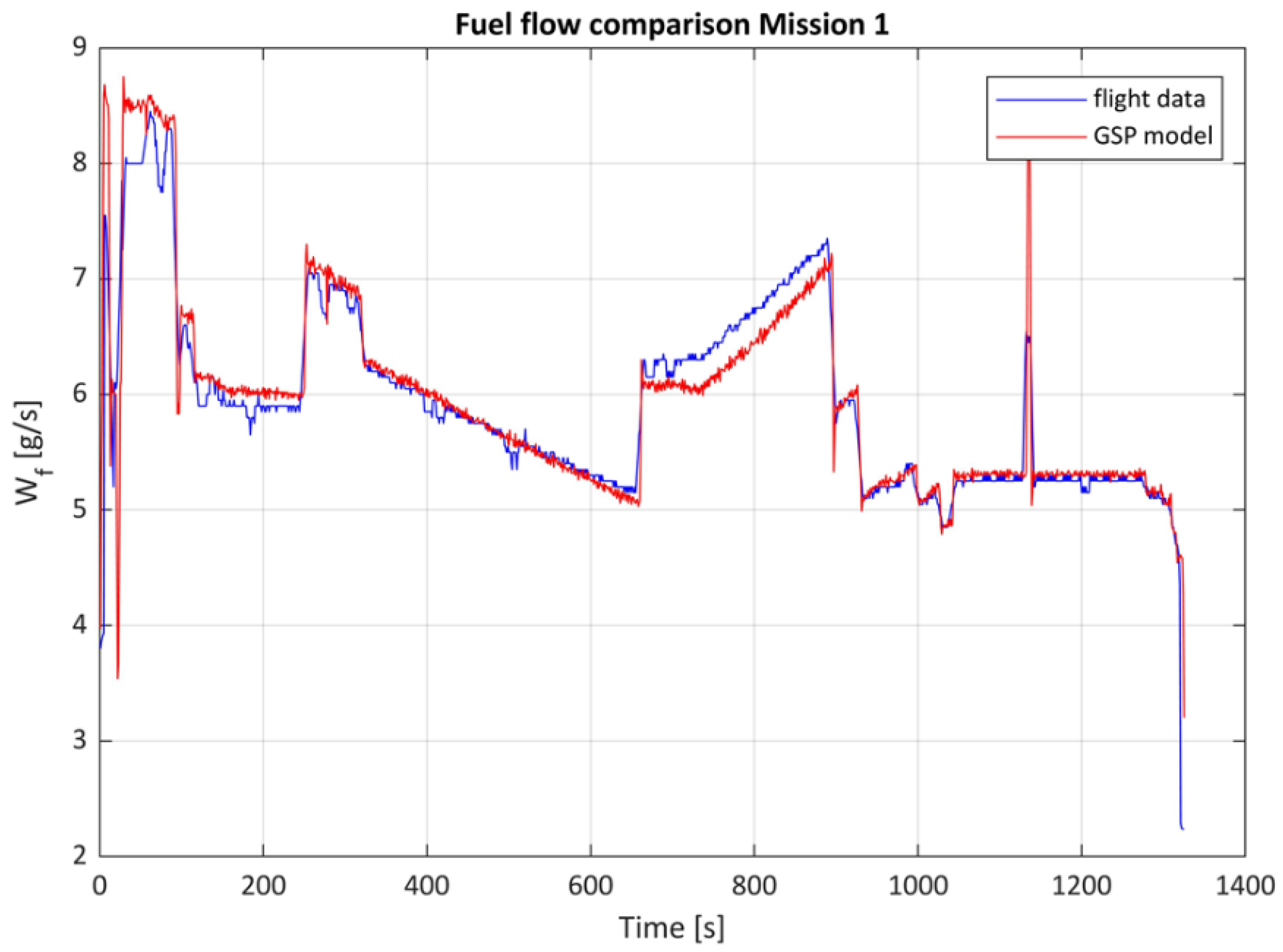
Validation of the model with the experimental data: The results of the steady-states simulation were compared with the test rig data of the reference microturbines. The comparison was made for different operating points referring to the in-flight engine operating range, even far from the design point, and with respect to various performance parameters (thrust, fuel flow, EGT, inlet air flow). The transient model was validated using data recorded by flight telemetry for four different missions, by comparing the EGT and fuel flow parameters.
2. Materials and Methods
2.1. Engine Specification
This research is based on extensive data gathered from test bench experiments and flight missions of a twin-engine target drone. Two types of micro turbojets were tested and modelled in this work: the Polish JETPOL GTM 140 and the German JetCat P140 Rxi-B. The experimental data belong to two different microturbines of the same thrust class, the Polish JETPOL GTM 140 and the German JetCat P140 Rxi-B. Specifically, complete steady-state data were available for the former engine, while flight data for the latter. Both engines were controlled by their original Electronic Control Unit (ECU), which was not modelled here.
Table 1 shows engine specifications. Looking at the values in the table, it is evident that the engine parameters are almost identical, except for the Engine Compression Ratio and the Design Maximum speed, which depend on design choices. The performance at the design point is very similar as well.
It is noticeable that the performance of both engines is very similar, and the data available complement each other, providing all the necessary information to create a microturbine transient engine model that can be reliably validated. From the above observations, the following assumptions for implementing the engine model were taken:
Maximum shaft speed (at Design Point) was set to 125,000 rpm, like for the JetCat P140 Rxi-B;
Bench test measurements and the map scaling factor was derived from the JETPOL GTM 140;
Transient performance was equal to those of JetCat, measured during flight missions.
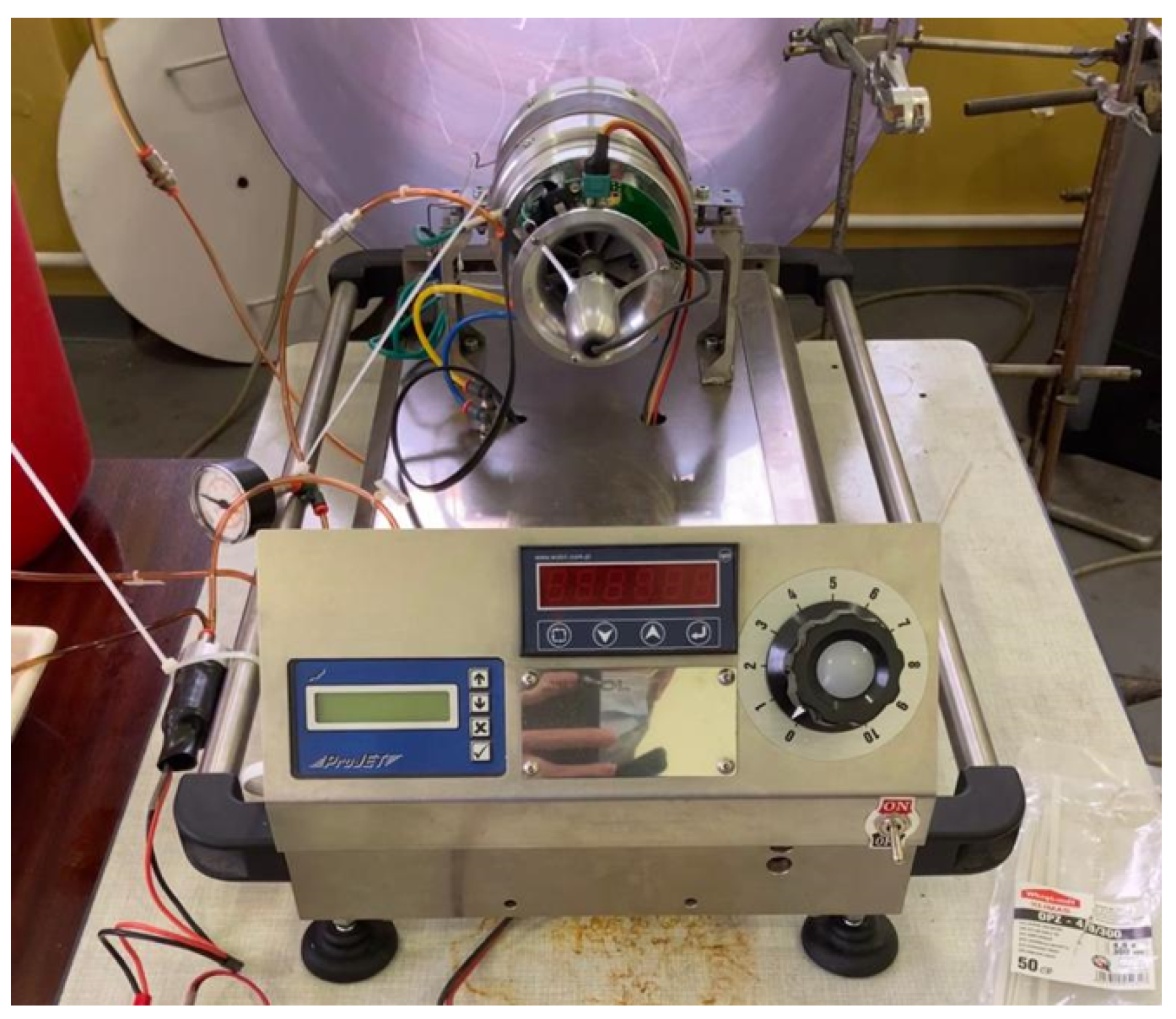
2.2. Test Rig Data
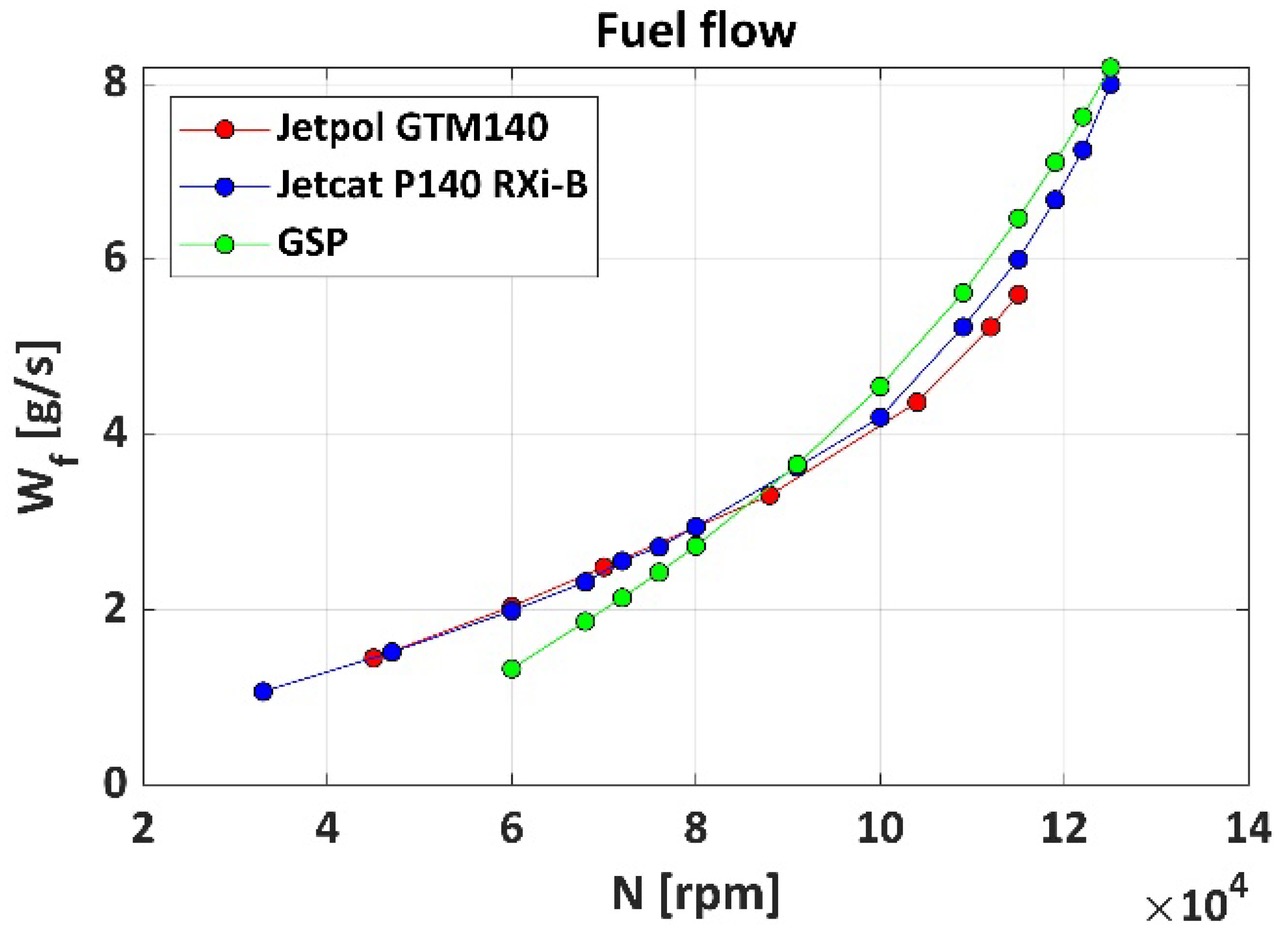
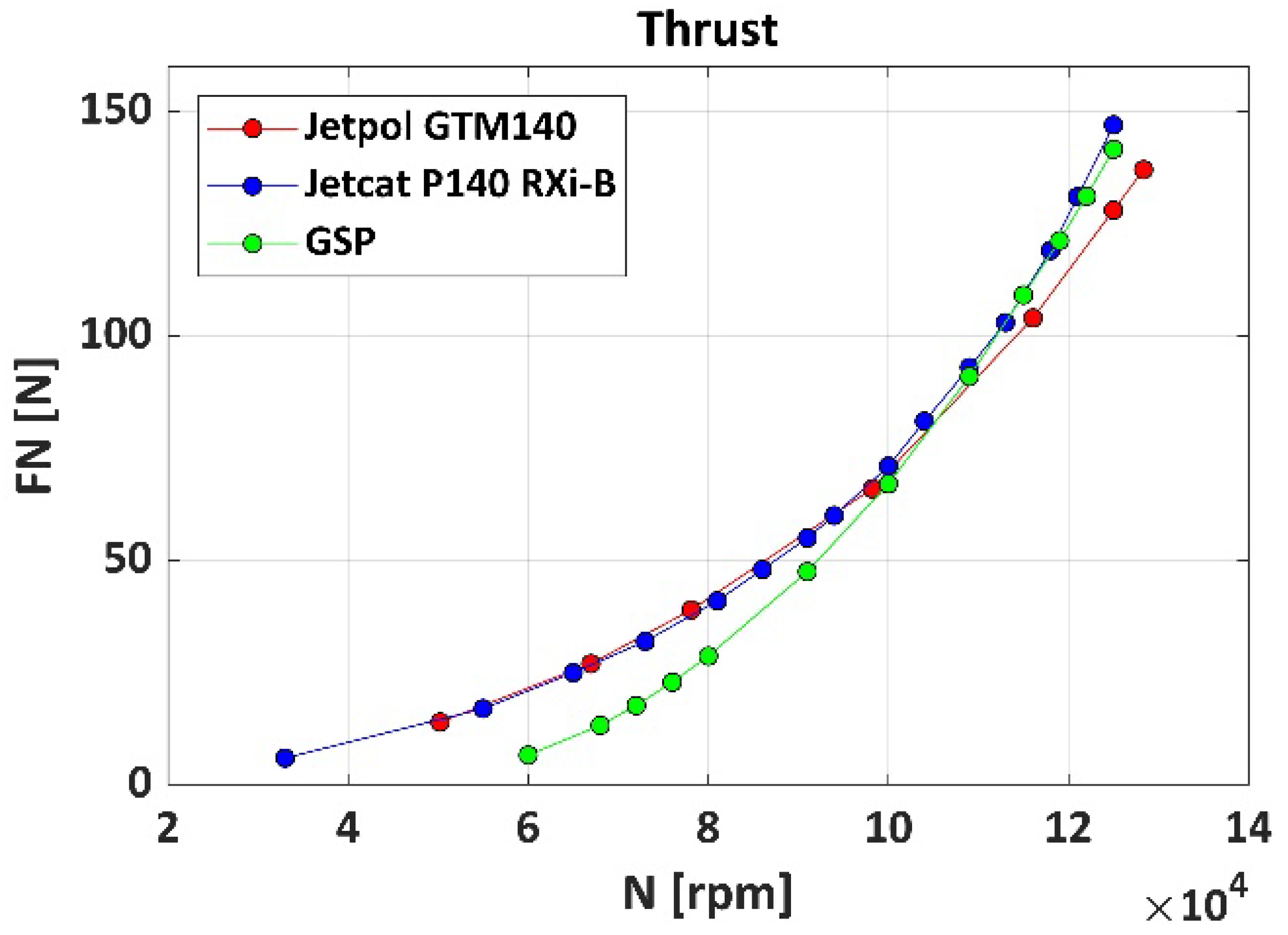
For JETPOL GTM 140, test rig measurements [
59] of temperatures and pressures at various engine stations, Exhaust Gas Temperature, air and fuel mass flow rate, and thrust were made at several shaft speeds (
Figure 1). For JetCat P140 Rxi-B, a bench test measurement [
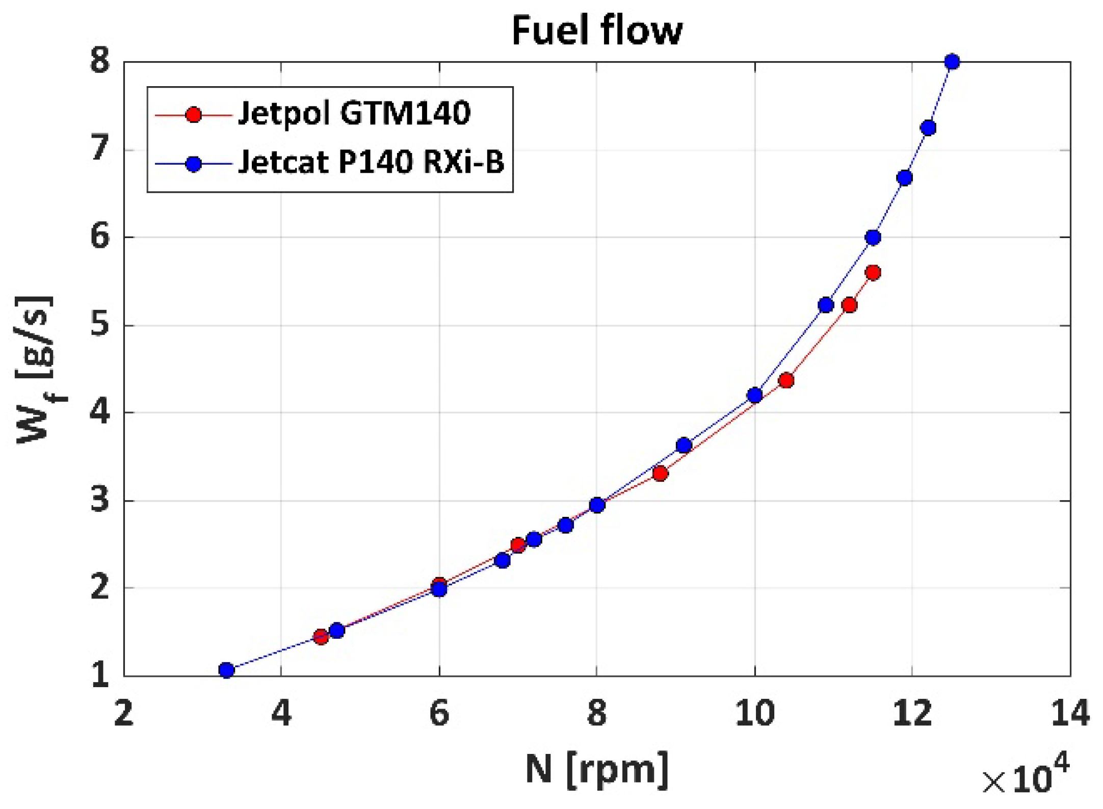
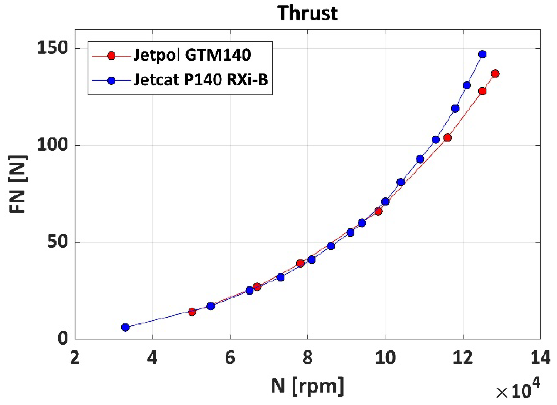
60] of thrust and fuel flow was provided at different shaft speeds. When comparing these two last parameters (
Figure 2 and
Figure 3), it is noticeable that the performance of the two engines is in good agreement. These two engines are not identical but their key components have the same geometry. There are significant differences in engine accessories, controls and instrumentation.
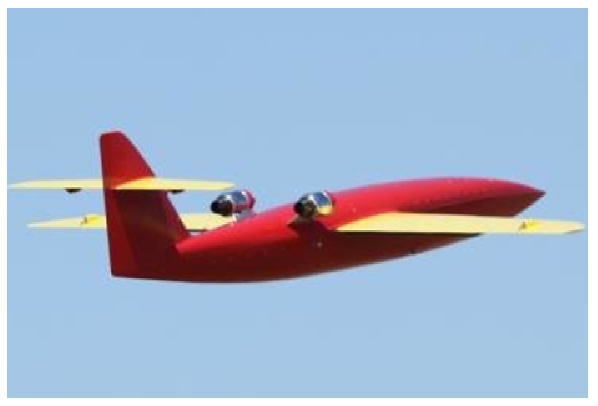
2.3. Flight Data
A prototype aerial target (
Table 2,
Figure 4) propelled by two JetCat P140 Rxi-B engines was flight-tested by the Air Force Institute of Technology (ITWL) in Poland [
60,
61]. In this work, flight data with a diverse mission profile were selected. The datasets represent a wide range of engine operations, so are well-suited for the effective validation of the engine transient model.
The following parameters were sampled with the rate of 50 Hz and were acquired via a telemetry system [
62]:
Air speed
Ambient temperature
Altitude
Shaft speed
EGT
Fuel flow
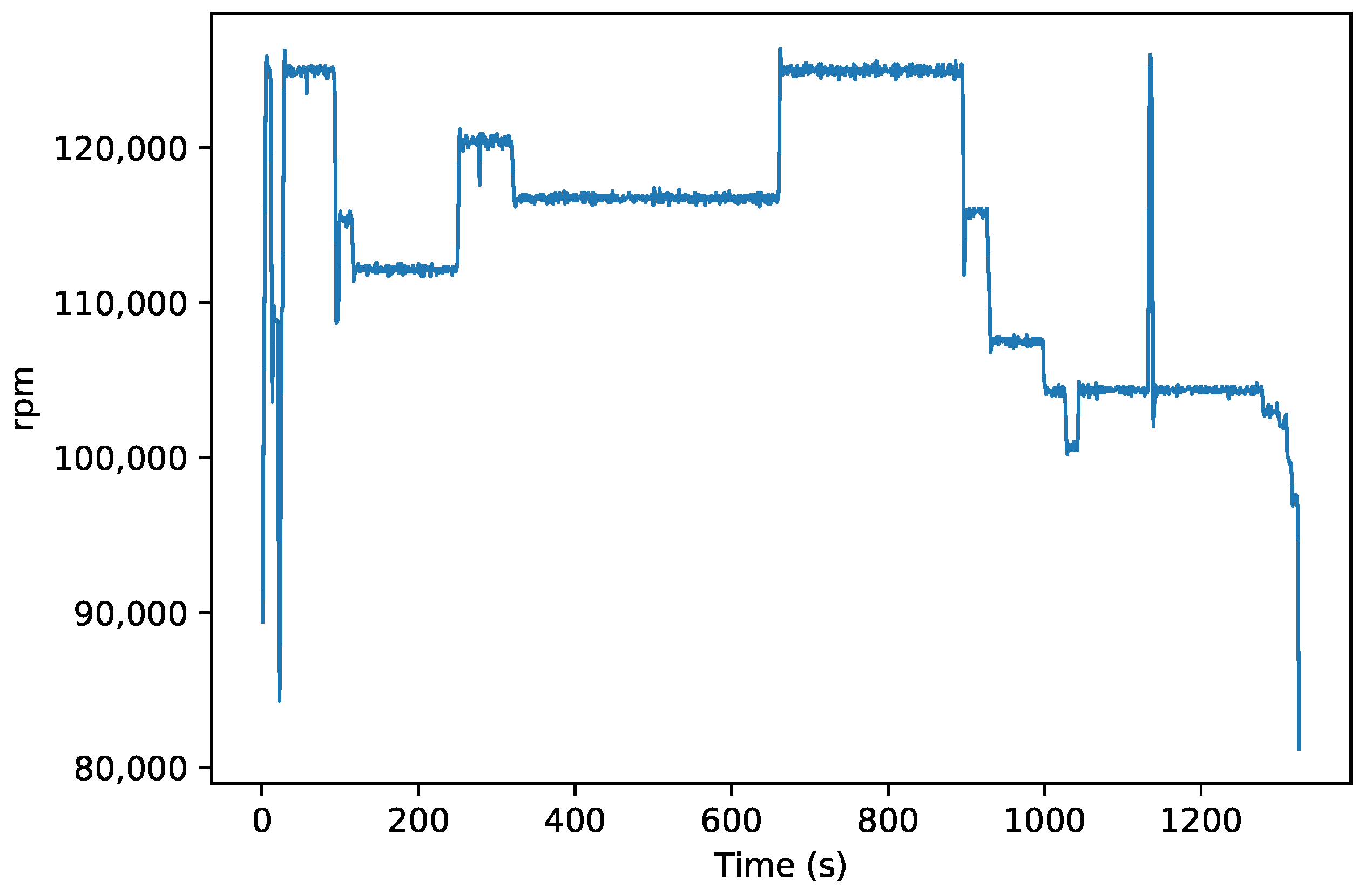
For a 30-min flight, the dataset is a table of about 90,000 rows, each of them representing a time step for which solving the system of equations, leads to prolonged computation in GSP. Furthermore, the recorded data included long intervals before the start and after the end of each flight. Those portions of the dataset, if included in the input, could completely invalidate a simulation process. Two approaches were used to reduce this amount of data: (1) bringing the sample rate down to 1 Hz; (2) considering only the data with engine speed greater than 80,000 rpm because it never went below this threshold during flight operations. Consequently, the irrelevant records were removed from the dataset that corresponded to the moments:
before take-off, when the engine idled but the aircraft had not been launched yet;
after the end of the mission, when the parachute opened, the engine idled and was shut down after a while. The recording ended either when the telemetry was turned off or when the target drone was recovered.
The data reduction was considerable (
Table 3).
2.4. Compressor and Turbine Maps
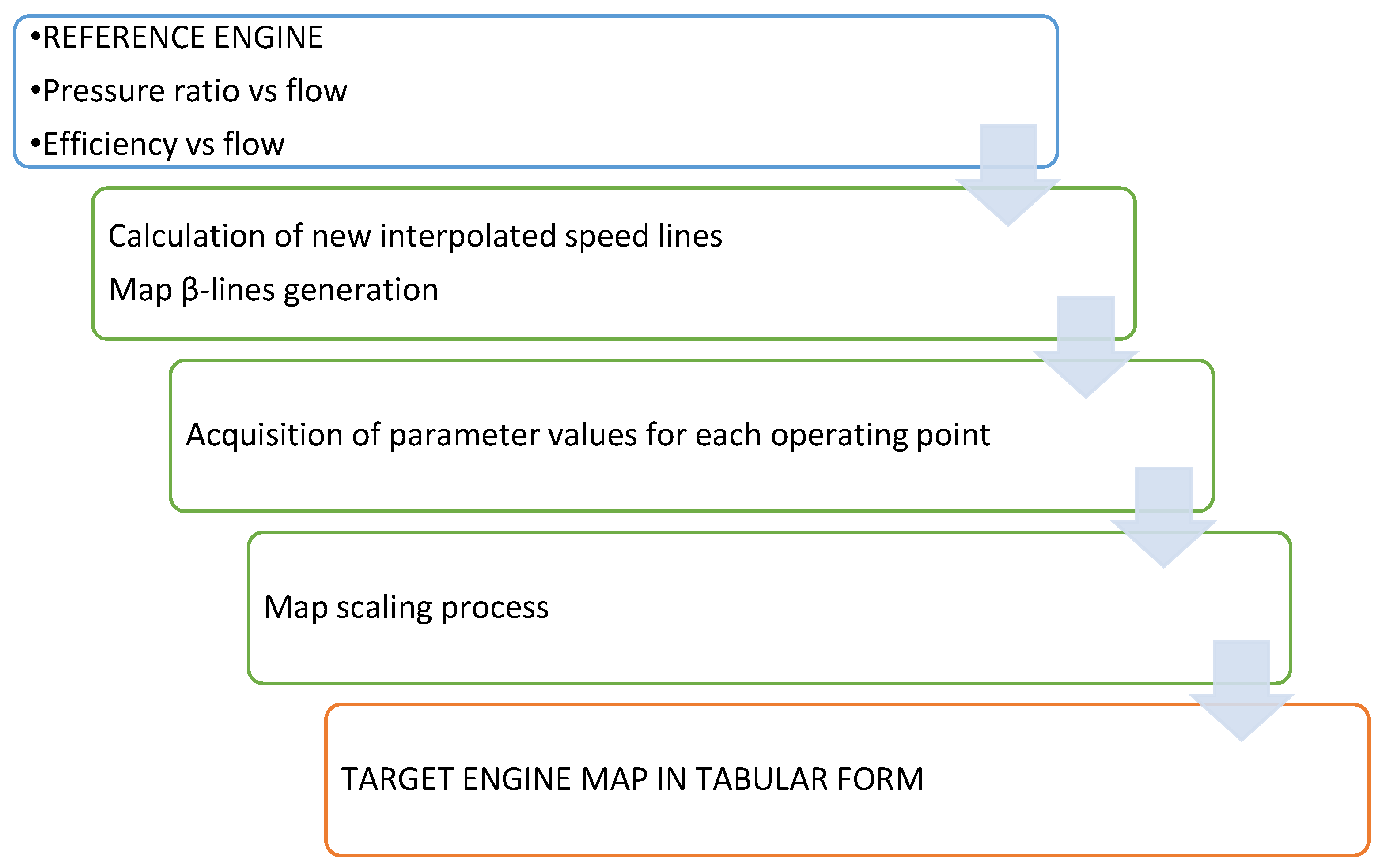
It was necessary to build new compressor and turbine maps in this work since the generic maps included in the libraries of GSP and GasTurb were not appropriate. This process is presented in
Figure 5. Our maps were generated using performance plots of a compressor and turbine provided by Rzeszow University of Technology, produced with CFD for a microturbine of similar geometry. For each component, there are two maps in the form of a bitmap: (1) Pressure ratio versus Mass Flow and (2) Efficiency vs Mass Flow. Then Smooth-C and Smooth-T tools from the GasTurb package were used, to digitize the plots, generate new interpolated speed lines, and create
-lines. The source maps and MATLAB scripts for their transformation are documented in thesis [
63].
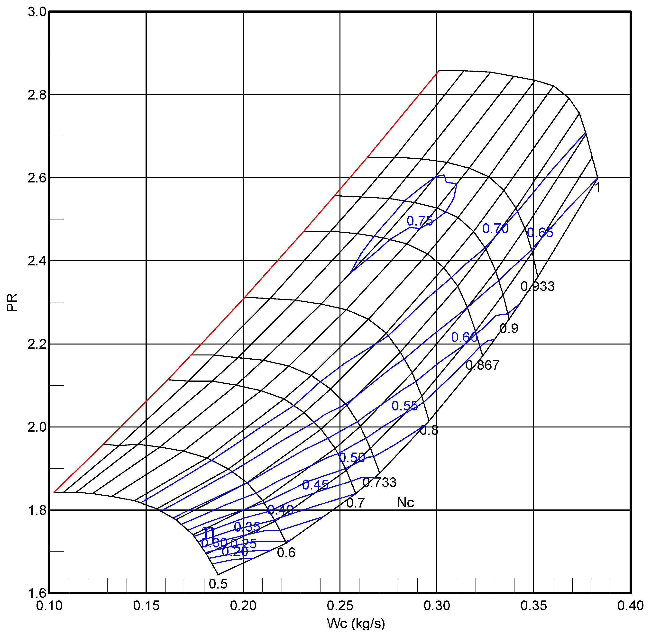
There are four parameters that are represented on a component map: (1) rotational speed; (2) mass flow; (3) pressure ratio (compression ratio for a compressor or expansion ratio for a turbine, respectively); and (4) efficiency. In addition, maps include -lines, which are a family of curves that do not have a physical meaning but they make it possible to uniquely define an operating point when speed lines in the graph are parallel to either the pressure ratio or the mass flow rate axis. The compressor map also includes the surge line which limits the area of its stable operation.
For the compressor, the Smooth-C tool was used, to digitize the plots, generate new interpolated speed lines, and create
-lines. In this way, for each operating point of the component, values of rotational speed, mass flow, pressure ratio and efficiency were found, defining them univocally. Some numbers regarding the results of the point acquisition can be found in
Table 4.
Then, single-point map scaling was attempted using the ratio of the design point value of the target engine and the design point value of the reference map. This was aimed at matching the values at the design point of the target engine without considering the differences on the other operating points. Unfortunately, this scaling failed since the model errors were above 40%, even when using radial compressor maps of similar sizes. Therefore, the alternative method known as applying factors and deltas was implemented. The least squares regression was employed to calculate scaling factors
and deltas
[
64], fed by a number of operating points obtained experimentally. The factors and deltas were then used to find the values of the scaled map:
For each map parameter, the values of more than two (four) operating points were considered, so that each of Equations (1)–(3) was an overdetermined system of equations with the scaling factor and delta as unknowns. Hence, as the name of the method suggests, these factors and deltas were obtained in a least square error sense. Although the scaled map does not exactly match the reference map, even at the design point, this method has the advantage of minimising the error between the different operating point data in the least square sense. The final target map can be found in
Figure 6.
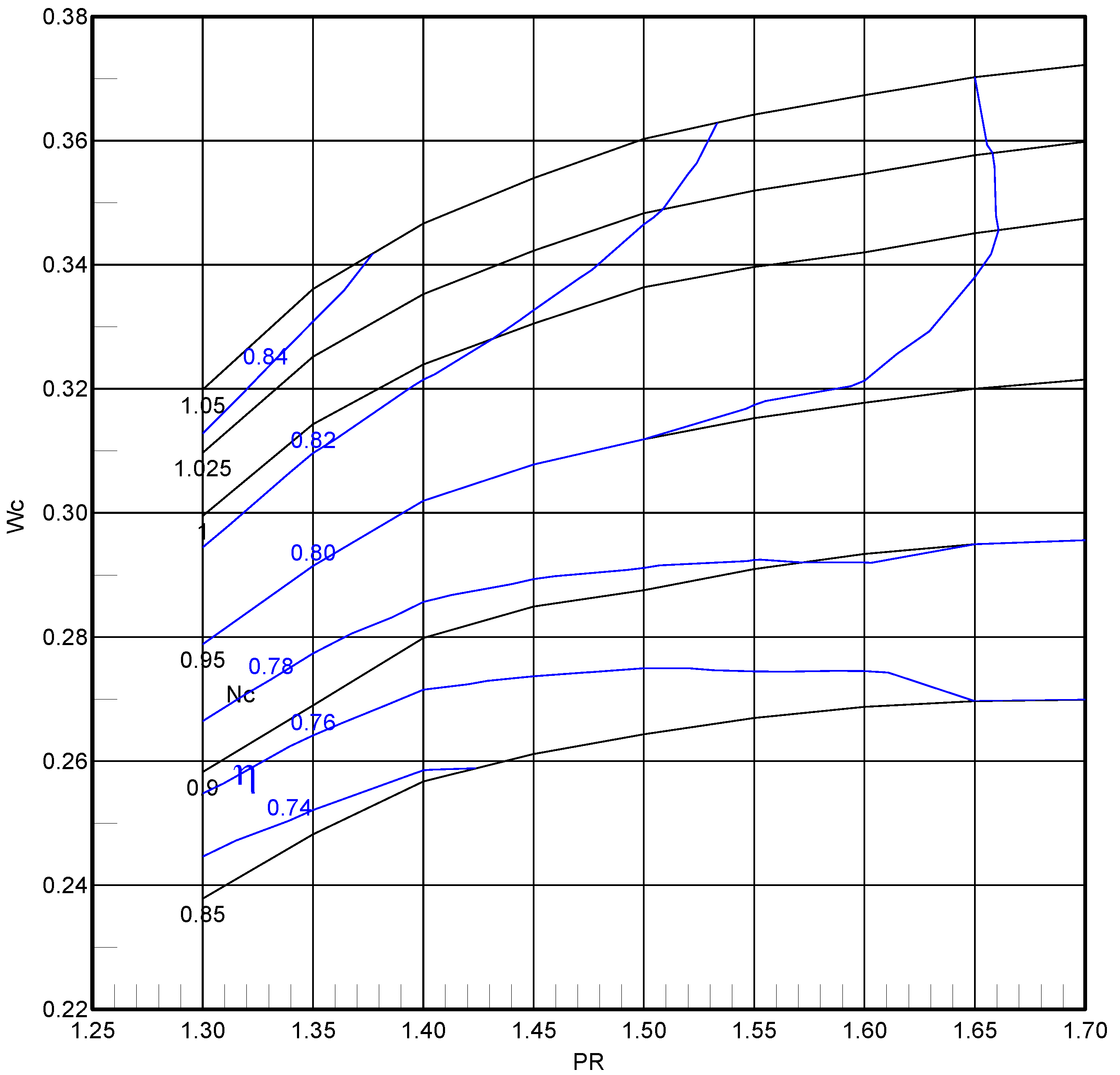
For the turbine, the Smooth-T tool was used to digitize the plots and generate new interpolated speed lines. However, in this case, instead of creating new
-lines, PR-constant lines were used as
-lines, because these were perpendicular to speed lines in the operating region of interest. Furthermore, no scaling process was required because the reference plots already had dimensionless parameters. The result can be seen in
Figure 7, and some numbers regarding the results of the point acquisition can be found in the third column of
Table 4. Finally, both maps written in the GasTurb tabular format [
63] were loaded into GSP.
2.5. GSP Model
The engine model was implemented in GSP, which is an object-oriented 0-D simulation environment [
57] in which averaged flow properties are calculated only at the inlet and exit of components while the flow field inside them is not analysed. GSP implements and integrates a set of non-linear differential equations describing the thermodynamic cycle and rotor dynamics [
65]. In particular, the acceleration or deceleration of the engine is the effect of power imbalance between the turbine and compressor:
where
and
are turbine and compressor power,
I is rotor’s moment of inertia and
is rotor angular speed.
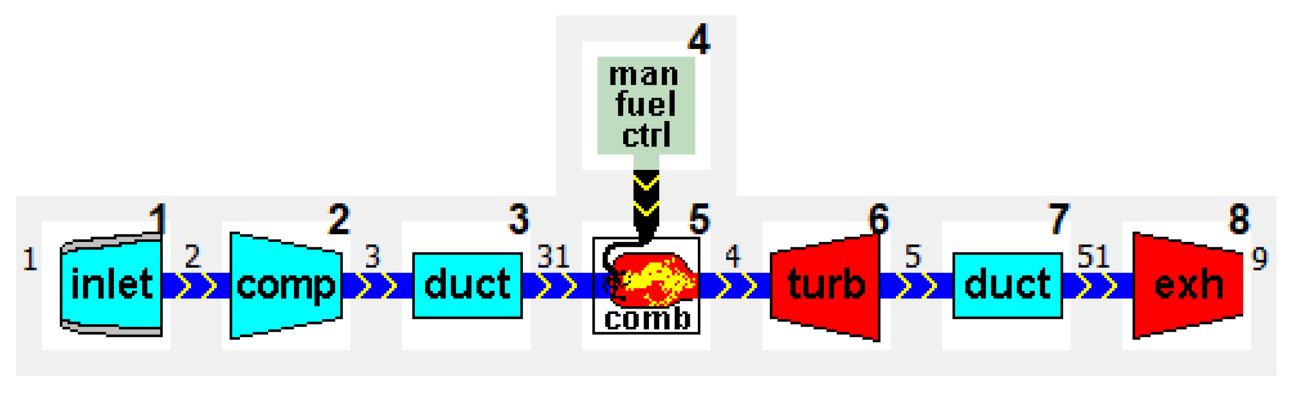
The adopted structure of the engine model (
Figure 8) follows the standard turbojet template with two Duct components added after the compressor and turbine, which was necessary for transient simulation. All the components were configured to accurately model the engine behaviour by setting their design parameters, such as the maximum speed, pressure ratio, mass flow rate, fuel flow rate, efficiencies and so forth.
4. Discussion
The performance modelling of full-scale engines has well-established methodologies and tools. However, they are not perfectly suited for micro turbojets, so their modelling may pose a challenge despite the basic structure of these engines. A full-size turbojet model cannot be simply scaled-down to a microturbine due to significant differences in efficiency and completely different dynamic response. Here, it was confirmed that library maps scaled at design point led to large model errors. Other minor issues were encountered e.g., the rotor’s moment of inertia was close to the minimum value allowed by GSP (10
kg m
). Due to very low inertia of the microturbine, the dynamics of transient responses observed in the experimental data were highly affected by sensors and the engine control system, which were not modelled here. The acceleration visible in
Figure 12 at t = 1135 s took only a second, which is a negligible time when compared to a full-scale turbojet.
The correct simulation of off-design and transient operation needs compressor and turbine maps that accurately describe the performance of the component over a wide operating range. To describe the component without significant errors, the reference map must refer to a component that is quite similar to the one under analysis, especially in terms of geometry; furthermore, the number of operating points and the scaling method must be sufficient. The maps and model implemented here better describe the engine in the upper speed range used in flight but they are less precise in the low speed region. The reason for this was the low detail of source map plots there i.e., low number of speed lines, related to the general difficulty of modelling compressors and turbines at low speeds. The problem of map extension to zero speed was recently addressed by Kurzke [
66] and Ferrer-Vidal et al. [
67].
Scaling the maps based on the least squares regression was sufficient and much simpler and faster than the adaptation of maps using the nonlinear optimization method [
68,
69]. Adaptive modelling methods [
70,
71,
72] will, however, be necessary for monitoring a fleet of engines with significant manufacturing tolerances or varying degrees of wear.
Considering that:
Measurement uncertainty at a microturbine is not as low as the uncertainty at a full-scale engine due to the small size of sensors and lack of space for them;
Performance can vary significantly from one engine to another due to its low cost that implies higher manufacturing tolerances of components;
Model is zero-dimensional (0D) and does not take into account the geometry of engine components;
Component maps were produced by CFD analysis for another micro turbojet because the actual geometry or experimental compressor and turbine maps were not available for both analysed engines;
the created GSP engine model showed satisfying results when compared to real flight data, with an average error of each output parameter under 5%. Therefore, it can be concluded that the model was validated.
Although it is not generally recommended, developing one model for two different designs was successful here because both compressors and turbines were almost identical. Thanks to this similarity, the difference in performance between JETPOL GTM 140 and JetCat P140 RXi-B was negligible, similar to the one related to manufacturing tolerances. For this reason, the developed model satisfactorily simulated the steady-state and transient operation of both engines. Its validation was a first step to implement a Digital Twin of the microturbine.
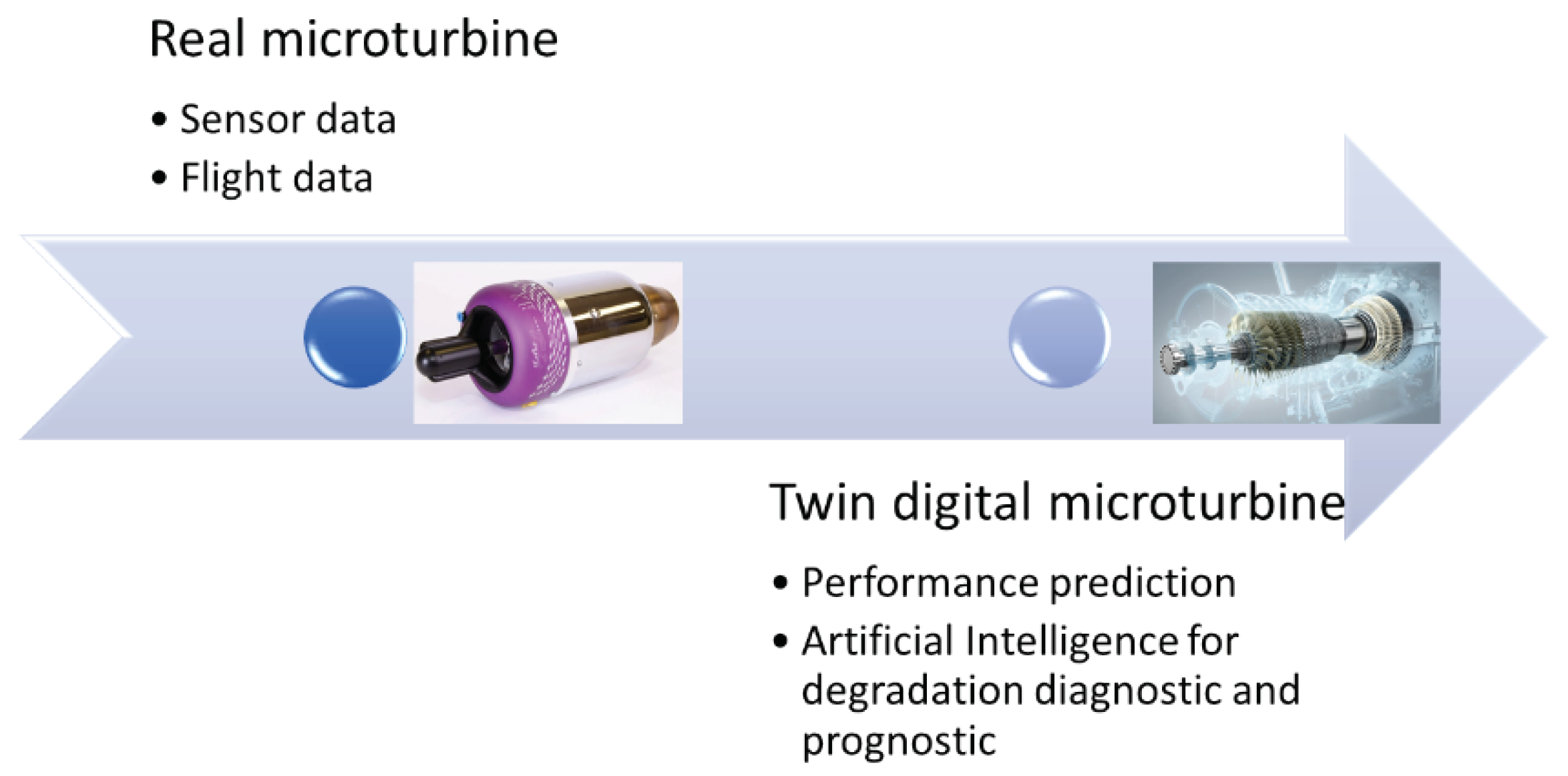
The digital twin model includes three parts: engine entity in physical space, digital engine in digital space, and data/information exchange between physical space and digital space (
Figure 15). This virtual engine is a high-fidelity integrated model that dynamically modifies its digital model in real time with the help of real-time data to ensure that its prediction accuracy is close to the reality. Model-based and data-driven fusion methods are essential for the core technology of digital twin model.
The digital engine model will accurately predict the engine performance such as thrust, fuel consumption and emissions, as well as will have the ability of degradation and fault diagnostic and prognostic based on operational data. Engine degradation will be implemented by setting a variation of the isentropic efficiency, the mass flow capacity and the pressure ratio for each level of degradation severity [
47]. Then the corresponding change of measurable variable (pressure and temperature) will be estimated. In this way a machine learning algorithm can be applied that based on operating conditions and measurable parameters such as pressure, temperature and rotational speeds can predict the health state conditions of each engine component. The algorithm will predict the component deterioration parameters and the level of degradation by a comparison with the healthy (no degradation) engine values, as well as the degraded performance in terms of thrust and specific fuel consumption.
The physics-based approach based on numerical simulation methods, such as 3D CFD calculations, can be expensive in terms of computing resources and time. Hence the 0D model, as the one implemented in this work, has advantages in computational time and can be used to simulate the engine in real time. The model-based approach has the advantage of being able to reflect physical processes. However, the implementation of physics-based engine model is complex and it is not perfectly suited for the prediction of slow degradation. In this case the data-driven method is more suitable and make it possible to estimate the engine performance according to the sensor data, even if the physical constraints and interpretability are weak. By using an hybrid approach employing physics-based and data-driven models [
52], the digital twin model of the microturbine based on 0D performance model and flight data will lead to accurate performance monitoring and life prediction. Furthermore, the model will permit a self-optimization ability to reduce fuel consumption when cruise and increase thrust when climb.


