1. Introduction
Reducing anthropogenic climate change is one of the most significant existential challenges that we face, and it requires a strong global response to, e.g., avoid tipping points [
1]. Aviation, for instance, contributed to 3.5% of anthropogenic climate change in terms of Effective Radiative Forcing when contrail-cirrus effects were included [
2] and 5% in terms of temperature change [
3]. Aviation climate impact is expected to grow rapidly due to the growth of the air transport sector in most regions of the world. The 4.3 billion airline passengers carried in 2018 are expected to grow to about 10 billion by 2040, and the number of departures is projected to rise to some 90 million in 2040 [
4]. Airbus [
5], in its Global Market Forecast, predicts a continued annual growth rate of 4.4% in revenue passenger kilometres for the next two decades. Boeing [
6], in its Commercial Market Outlook, expects an annual growth rate of 4.6% per year. The effects of the COVID-19 pandemic are expected to only have a temporary effect on this growth [
3].
Although efforts have been made to reduce fuel consumption (and hence reduce the CO
emissions) with technological, operational and regulatory measures, they are not sufficient to tackle the overall climate impact of aviation. This is because non-CO
emissions from engine fuel combustion contribute to about 2/3 of the warming [
2] in terms of Radiative Forcing (RF) with large uncertainties for contrail-cirrus effects. The most important non-CO
emissions include persistent line-shaped contrails, contrail-induced cirrus clouds and nitrogen oxide (NO
= NO + NO
) emissions that alter the O
and CH
concentrations, both of which are greenhouse gases, and the emission of water vapour (H
O).
It is important to understand the fundamental differences between CO
and non-CO
effects in order to predict the overall climate impact of aviation. The climate impact of CO
is proportional to the quantity of CO
released during the flight and, as CO
is a long-lived and relatively well-mixed gas, the impact is independent of the emission location. Additionally, the climate impact of CO
has been determined with a high confidence level. On the contrary, non-CO
emissions and contrail cirrus have shorter atmospheric residence times and are heterogeneously distributed. For each non-CO
emission, it is not just the individual concentration that is important but also the location of the emission, the associated timescale, chemical background condition, etc. [
7,
8,
9]. Consequently, the confidence levels are much lower and associated uncertainties are much higher for these non-CO
effects (Figure 3 of [
2]).
Because non-CO
effects show strong spatial and temporal variations, the weather situation and subsequent transport pathways play a major role in their climate impact. Accordingly, operational measures such as climate-optimised flight planning can be enforced to avoid regions where these impacts are substantial. This was the primary motivation behind the Reducing Emissions from Aviation by Changing Trajectories for the benefit of Climate (REACT4C,
https://www.react4c.eu/, accessed on 20 October 2021) project [
10]. The project led to the development of Climate Change Functions (CCFs, [
9,
11]) that can quantify the climate impact for a unit emission at a given longitude, latitude, altitude and time. The effects take into account the CO
emissions and non-CO
effects from the NO
and H
O emissions and contrail formation. The CCFs describe “climate sensitive regions” which are 4D regions in space-time, indicating where aviation emissions have a larger impact on climate change in comparison to other regions. The CCFs were used in an air traffic optimisation routine to avoid climate-sensitive regions and quantitatively showed a reduction potential of up to 25% in climate impact for a small increase in cost (0.5%, [
12]). However, these results were computationally intensive to generate in the first place and also restricted to the Trans-Atlantic airspace. This makes the practical use of these tools in climate-optimised flight planning a major obstacle. As a following step, a more general and practical tool was sought while making use of the vast amount of CCFs data, which was one of the objectives of the Air Traffic Management 4 Environment (ATM4E,
https://www.atm4e.eu/, accessed on 20 October 2021) project. Among other things, this project explored the feasibility of a concept for environmental assessment of ATM operations working towards environmental optimisation of air traffic operations in the European airspace [
13]. The project led to the development of algorithmic Climate Change Functions (aCCFs) separately for the NO
effect on O
(NO
-O
) and methane (NO
-CH
) (Sections 4.3 and 4.5 of [
14], respectively), water vapour (H
O) (Section 3.3 of [
14]) and contrail cirrus [
15], and the aCCFs are implemented as a submodel [
16] in the ECHAM5/MESSY Atmospheric Chemistry (EMAC) model [
17]. These formulas, obtained using regression techniques, are computationally inexpensive, fairly general and provide the climate impact based on meteorological inputs, in terms of a metric called F-ATR20 which gives the Average Temperature Response over a time horizon of 20 years given future increasing emissions (e.g., Fa1 scenario, [
18]). With these salient properties, the prototype aCCFs are expected to be used to optimise flight trajectories (in real time) with respect to its overall climate impact (CO
and non-CO
) and also to estimate the climate impact of individual flight trajectories. A general comparison between the characteristics of the CCFs and aCCFs is listed in
Table 1.
The quality of the aCCFs are expressed in terms of the adjusted
[
19]. This value is large for H
O aCCFs, but for O
aCCFs and CH
aCCFs, it is much smaller [
14]. A strict verification process for the aCCFs is required in general and this study focuses specifically on the O
aCCFs evaluation.
NO
(=NO + NO
) is an indirect greenhouse gas that leads to a short-term increase in tropospheric O
production (warming) and a long-term increase in CH
oxidation (cooling) in the atmosphere. Because CH
is a precursor for changes in O
, a long-term reduction in O
called the primary mode ozone (PMO) effect [
20] occurs due to CH
oxidation, resulting in cooling. Additionally, less CH
enters the stratosphere, where it is decomposed into CO
and H
O. Eventually, this reduces the stratospheric water vapour (SWV), resulting in cooling [
21]. However, the net climate effect for this chain of reactions is warming [
22,
23,
24]. The short-term O
production from NO
starts with the formation of NO
from NO through the reaction with HO
. Through photolysis of NO
, O(
P) is formed which in turn forms O
. Therefore, the following reactions are included:
For further details on the chain of chemical reactions relating to CH
, the reader is referred to Rosanka et al. [
25]. The NO
effects are characterised by significant seasonal and spatial variability due to the dependence on incoming solar radiation and background chemical (especially NO
) concentrations [
26]. Frömming et al. [
9] found that not only the emission region is relevant; in fact, the main driver for the enhanced climate sensitivity is the transport pathways of emissions within the first week(s) after emissions are released. The transport pathways are in turn driven by the meteorological situation. The detailed impact of weather patterns and related transport processes on aviation’s contribution to O
is also reported by Rosanka et al. [
25].
Preliminary results by Yin et al. [
27] showed that climate-optimised flight trajectories considering only O
aCCFs reduce the NO
-induced O
RF. Here, we are aiming to extend it by following a more detailed optimisation procedure (treating lateral and vertical shifts) involving a large variability of O
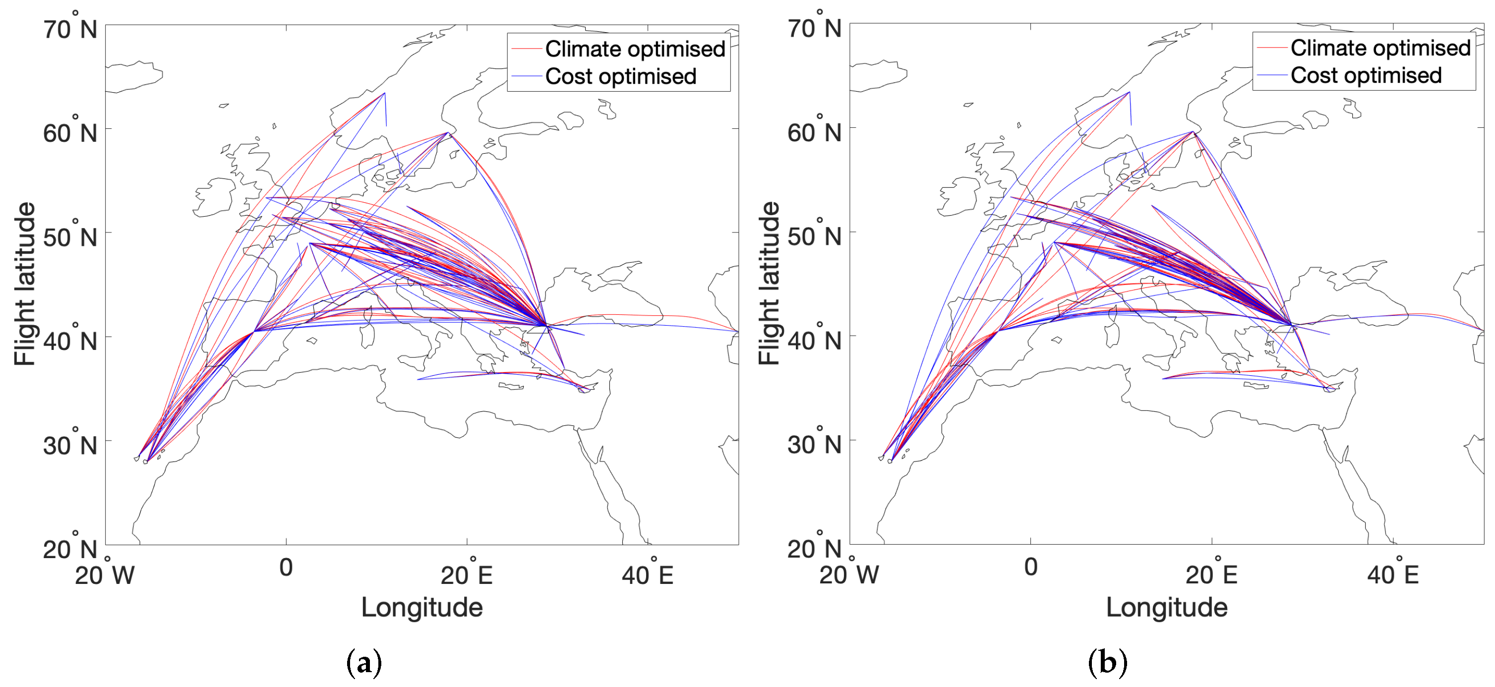
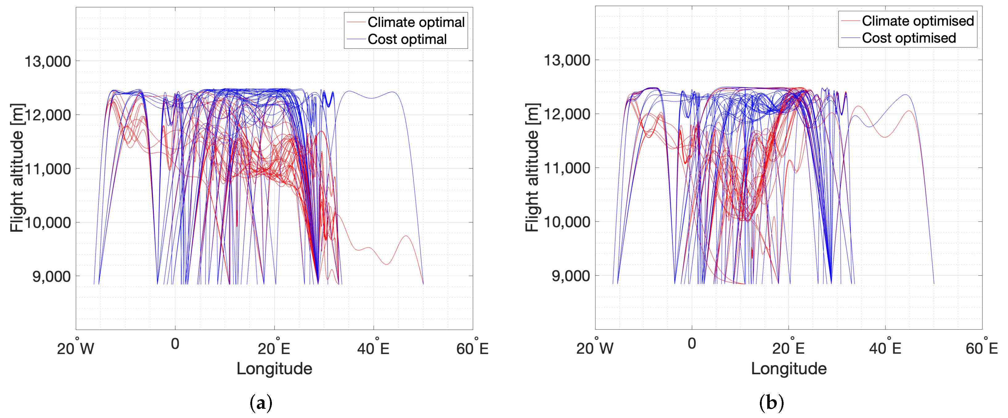
aCCFs. Hartjes et al. [
28] determined three-dimensional aircraft trajectories while minimizing contrail formation. They found vertical trajectory adjustments to be preferable over horizontal trajectory changes. This is an additional motivation to separately investigate the impact of lateral re-routing and vertical re-routing in relation to NO
-O
effects. As a result, it is possible to analyse different NO
emission profiles emerging from cost and climate-optimised simulations on days characterised by a large variability of O
impact. In order to test the ability to use the O
aCCFs for a reduction in O
-RF by trajectory optimisation, a summer day and a winter day characterised by a large variability of O
impact are selected. Subsequently, the atmospheric transport subject to meteorology and climate impact is analysed for all cases which are discussed in
Section 3. This leads to information on the viability of the O
aCCFs as a tool for obtaining climate-friendly trajectories as well as the impact of lateral and vertical re-routing.
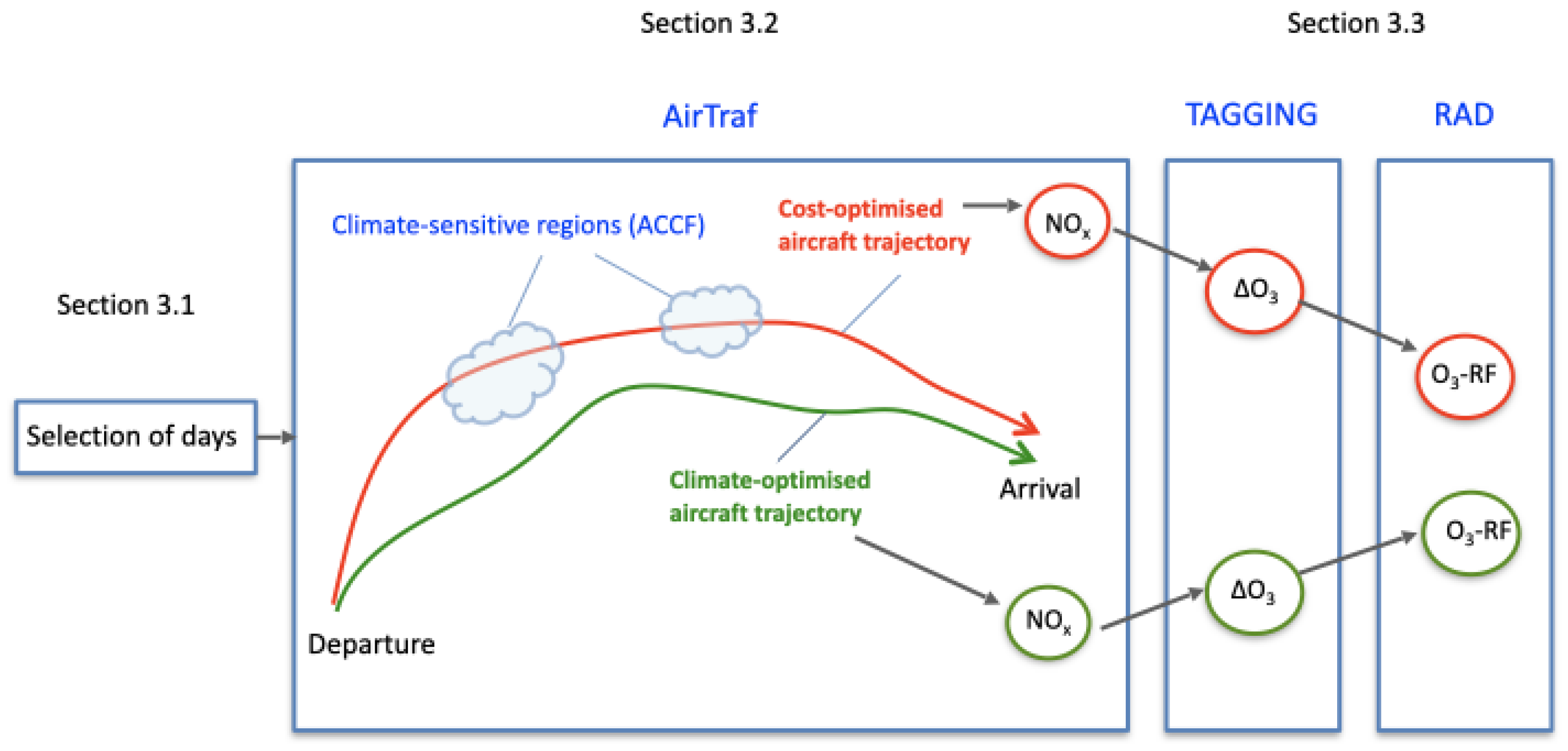
The present study is organised as follows: In
Section 2, we give an overview of the model system used and describe the applied setup in
Section 3. In
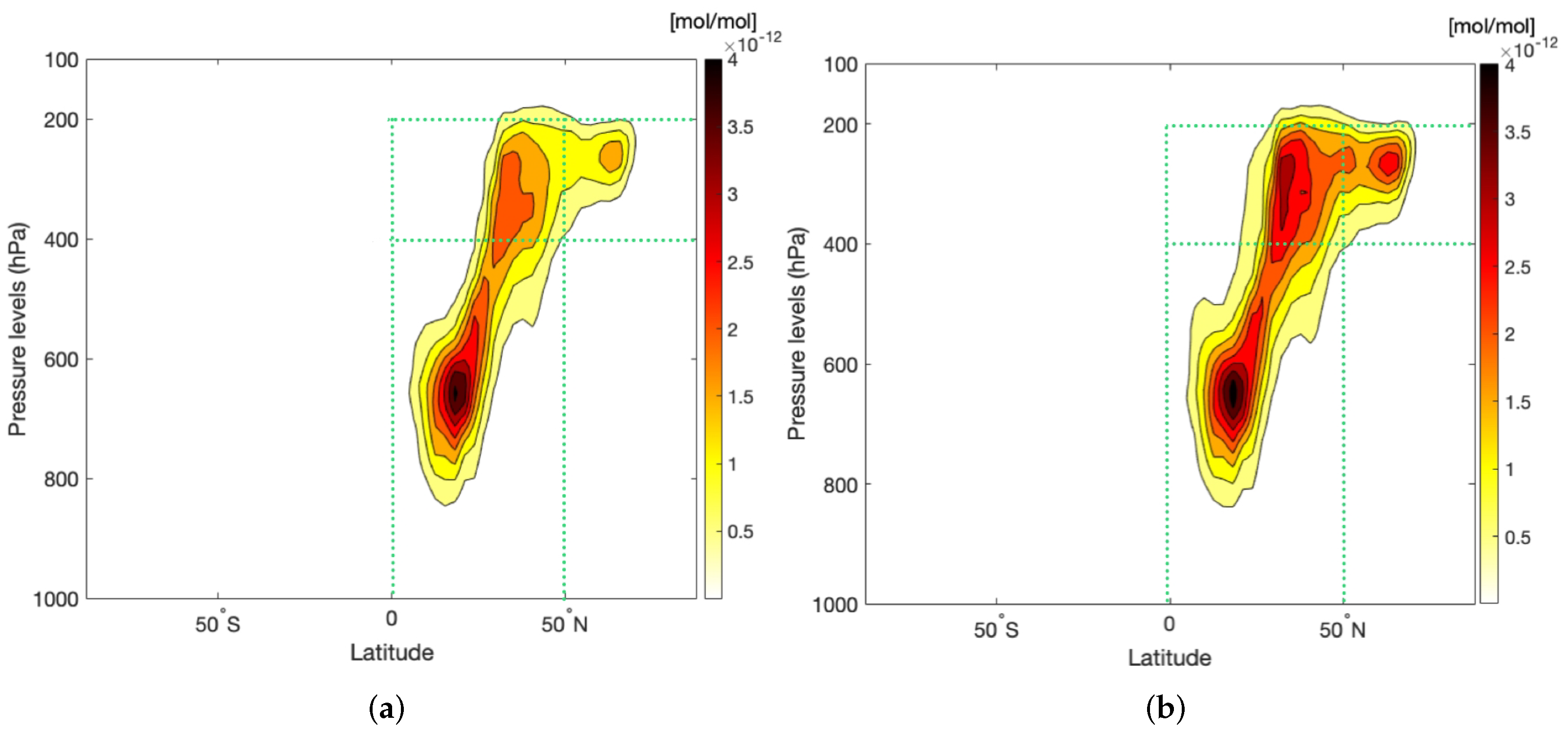
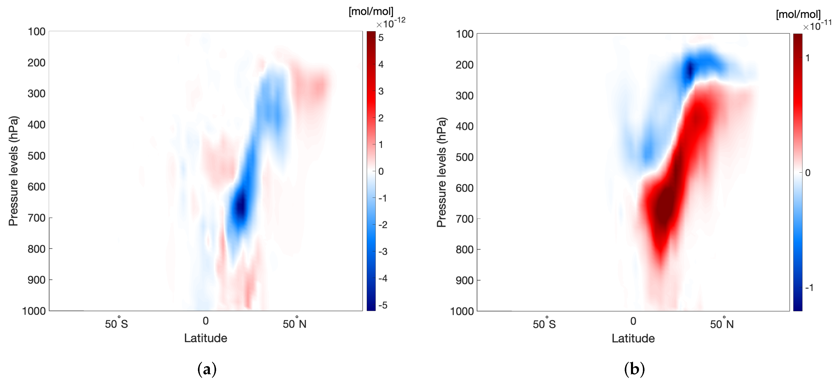
Section 4, we analyse our simulation results with respect to the contribution of NO
emissions from lateral re-routing and vertical re-routing on two selected days to tropospheric O
production and the resulting climate impact in terms of O
-RF. Here, a direct comparison of the climate impact from cost-optimised and O
aCCFs-optimised trajectories is made. In
Section 5, we discuss and conclude the present study.
5. Discussions and Conclusions
The possibility of reducing aviation’s overall climate impact requires us to take into account various non-CO effects such as HO, contrails, aerosols and NO effects on O and CH. This study looked specifically into short-term NO effects on O production, a phenomenon that is governed by several competing factors, such as emission location and time, synoptic situation, transport pathways and photochemical activity. The prototype O aCCFs were introduced as a tool to facilitate the prediction of O CCFs by means of instantaneous weather data (temperature and geopotential) without the need for the computationally expensive procedure of recalculating CCFs. However, this comes at a cost of larger uncertainties and lower accuracy, which necessitates a study to test its validity. Hence, the hypothesis was that O aCCFs can mitigate short-term aviation NO-O effects compared to cost-optimised flights for days characterised by a large spatial variability of O aCCFs.
It was shown that under large weather variability (
Section 4.1), O
aCCFs were able to generate more climate-friendly flights than the cost-optimised flights for the two specific weather patterns, thereby complying with findings by Yin et al. [
27]. The impact of the weather situation on the selected winter and summer days and the subsequent transport pathways proved to be very crucial in the climate impact of flights as was discussed in earlier studies (e.g., [
9,
12,
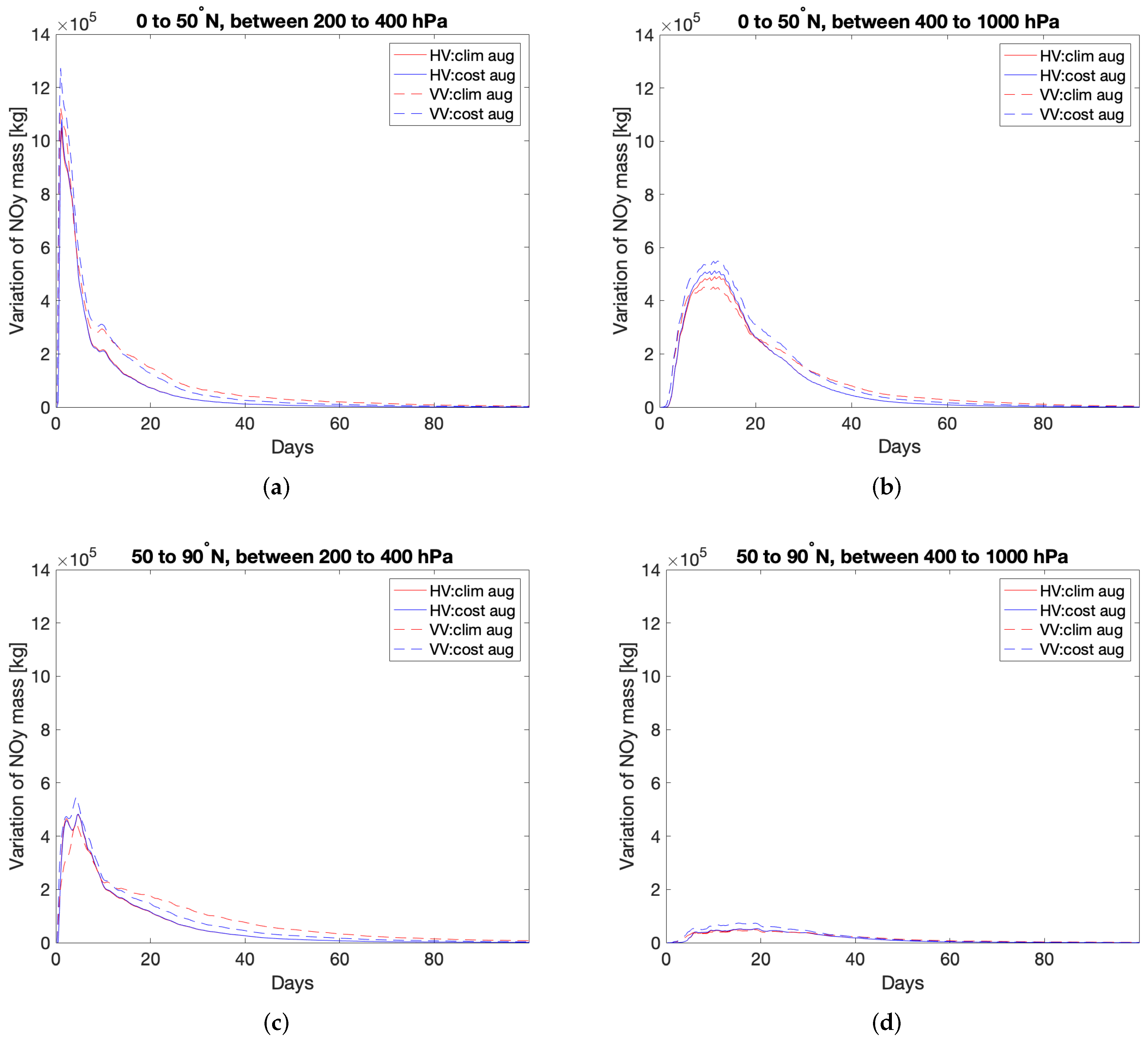
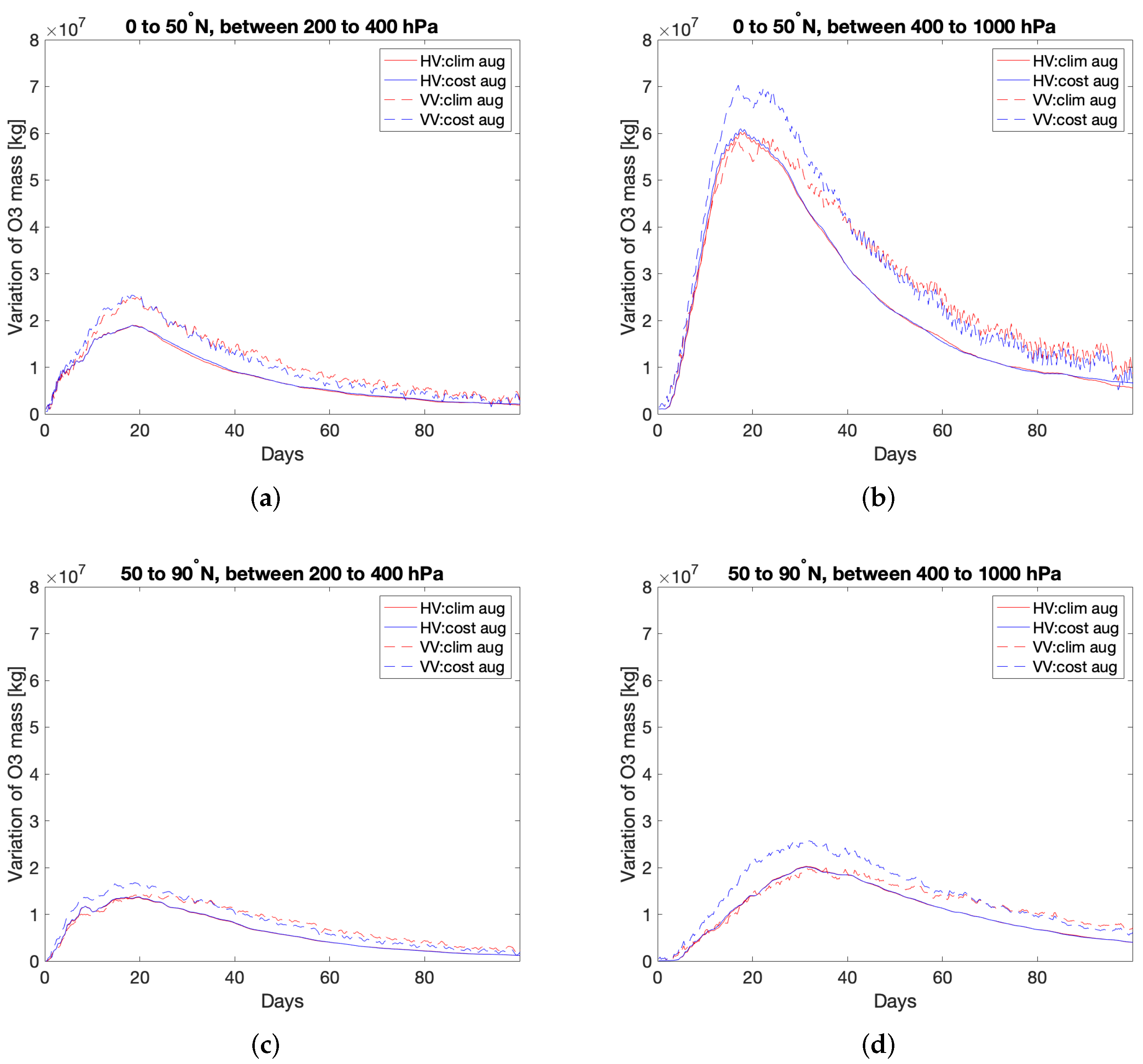
25]). While looking into detailed 1-day air traffic optimisation, it was found that, on average, for climate-optimised flights, there was a much larger deviation in vertical re-routing compared to lateral re-routing. Although laterally re-routed flights consumed more fuel and emitted more NO
than vertically re-routed flights, the climate impact was still lower. This can be attributed to the location and spread of NO
emissions and possibly the choice of cruise level. It would help extending the analysis to other cruise levels to test the sensitivity of O
production and the subsequent RF, as the corresponding findings can also be compared with other studies (e.g., [
57,
58,
59]). For vertically re-routed flights, the difference in the O
-RF between climate- and cost-optimised flights (and hence climate mitigation potential) was found to be larger than for laterally re-routed flights. Because the flight altitude was variable in this case of vertical re-routing, the NO
emissions were subjected to different chemical regimes. Additionally, the emissions were also driven by the transport pathway, causing a larger difference in O
production and, hence, RF. The NO
-O
effects were found to be stronger in the summer period than in winter, which also agrees with previous studies (e.g., [
25,
60]). Although those findings in general might apply to other seasons, future studies could check if there are any special features due to various photochemical regimes for NO
-O
effects. Additionally, NO
emitted at lower altitudes has a shorter residence time (e.g., [
56,
57]), resulting in a further reduction in climate impact for vertically re-routed flights for the selected summer day.
For the RF calculation for an O
perturbation, a more advanced radiation flux change is required than instantaneous RF at the tropopause, because it is not a reliable predictor for expected resulting temperature change [
61]. On the other hand, the simulation set-up employing pulse emissions is not well suited to derive stratospheric-adjusted RFs or effective RFs. To overcome this discrepancy, Grewe et al. [
11] and Frömming et al. [
9] applied a post-processing to their instantaneous RF values, converting them into stratospheric-adjusted RFs on the basis of a range of pre-calculated scenarios. However, a revision for this procedure might be necessary [
14]. Therefore, here, we decided to consistently apply the adjusted RF calculation (this value covers only a part of the stratospheric temperature adjustment, as a full adjustment could not be covered due to a simulation length of just four months) for the cost- and O
aCCFs-optimised air traffic, using the RAD submodel (
Section 4.4).
In the present study, we looked at flight optimisation in the European airspace, but it might help extending the analysis to the North Atlantic region where there is more freedom for routing to change: longer distances allowing detours and identifiable weather patterns [
53]. Finally, Frömming et al. [
9] took into account the influence of the weather on the total NO
CCFs. This total effect includes not just the short-term increase in O
but also a long-term decrease in CH
and a CH
-induced decrease in O
(PMO and stratospheric water vapour decrease). In order to take this total effect into account for arbitrary situations using aCCFs, the current CH
aCCFs need to be carefully evaluated [
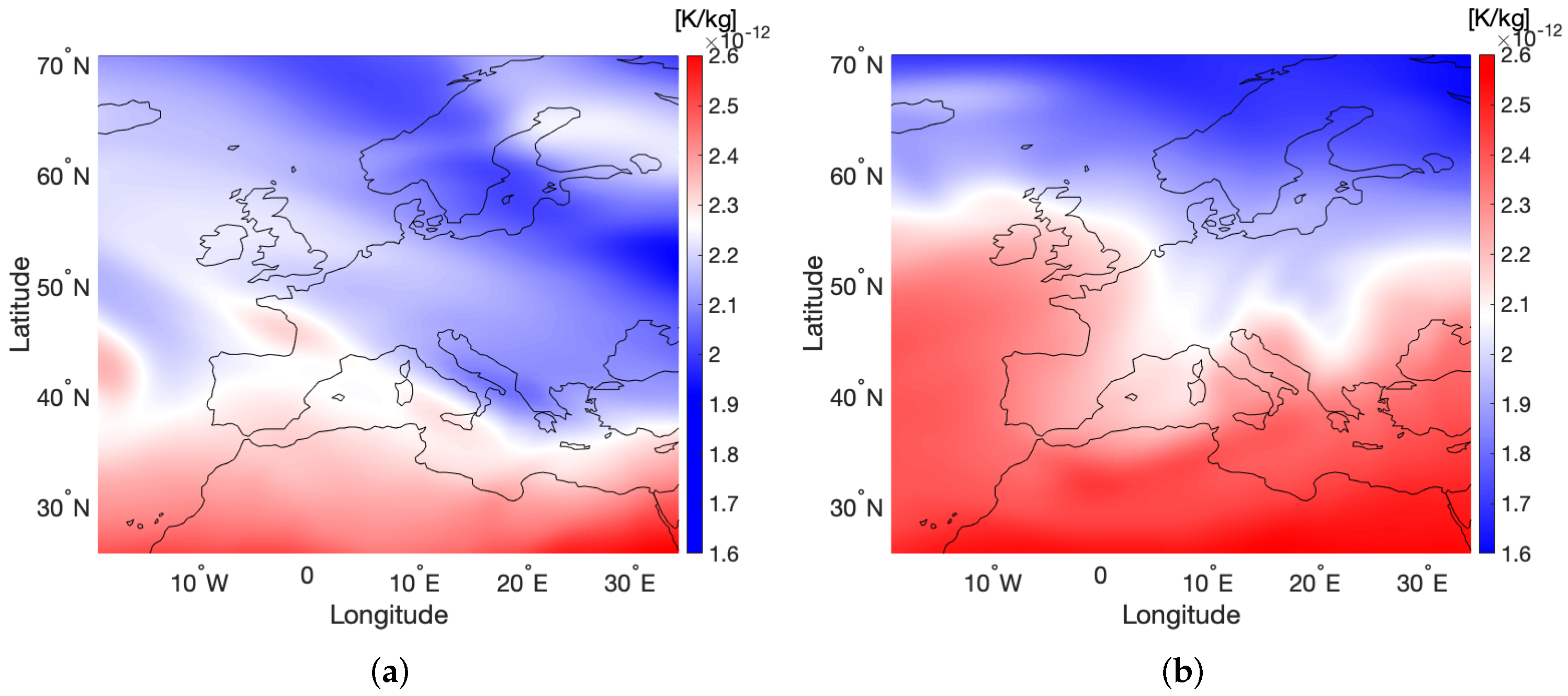
14]. Note also that there was a strong connection between the weather situation and O
CCFs as shown by Frömming et al. [
9], but the O
aCCFs do not capture all features equally well (
Figure 8b and
Figure 9). Hence, while the aCCFs in general are useful in calculating real-time flight trajectories for the sake of climate impact mitigation, looking at ways of improving them will lead to much needed improved predictions of climate impact from non-CO
effects of aviation, which are highly needed. We intend to do this by extending the CCFs and the consequent aCCFs to more regions, e.g., Africa, Australasia, Eurasia, North and South America, and to use more powerful statistical techniques. The use of the concept in daily operations seems to be feasible; however, it requires several steps to make it operational. Roadmaps have been outlined in
Figure 4 of Grewe et al. [
62] and
Figure 9 of Matthes et al. [
63] that comprise an investigation of uncertainties and robustness of such aCCFs concepts (see also Matthes et al. [
64]), impacts on air traffic densities and hot spots and the exploration of economic measures. As a result, climate-optimised flight planning could be practically feasible.


 ,
, 


