Abstract
Understanding the mechanism of the aeroelastic stability improvement induced by mistuning is essential for the design of bladed disks in aero-engines. In this paper, a quantitative interpretation is given. It starts by projecting the mistuned aeroelastic modes into the space spanned by the tuned modes. In this way, the mistuned aeroelastic damping can be expressed by the superposition of the tuned damping. Closed-form expressions are found, providing clear interpretations of several frequently reported trends in the literature. Further, a prediction approach is proposed, where the analysis of aeroelastic coupling only needs to be performed once, and it is decoupled from the analysis of the mistuning effect. The advantages are two-fold. First, the design of the mistuning pattern is accelerated. Second, this allows one to introduce more accurate data or models of aeroelastic damping. An empirical bladed disk with NASA-ROTOR37 profile is used as an example, and the alternate, wave, and random patterns are considered.
1. Introduction
Avoiding flutter is among the critical tasks in the design phase of bladed disks for modern turbomachinery. Although bladed disks are preliminarily designed to be tuned (with identical mechanical properties at each blade sector), in reality they are always slightly mistuned due to manufacturing error and in-service wear. Despite the risk of response amplification [1], mistuning is beneficial to the aeroelastic stability of bladed disks [2,3]. Since the aforementioned intrinsic sources of mistuning are almost random and uncontrollable, it is commonly suggested to intentionally impose a certain degree of mistuning to maximize the enhancement of aeroelastic stability. Experimental evidence can be found in the open literature, where researchers imposed mistuning by milling groove [4], heavy paint [5], and tip mass [6,7].
The deviation rule of mechanical properties among blade sectors, also known as the mistuning pattern, plays an important role in the enhancement of aeroelastic stability. The most frequently investigated mistuning pattern is the one in which the odd and even numbered blades have different modal frequencies for the same modal shape (e.g., bending or torsional). This is known as alternate mistuning [1], and its performance is better than randomly choosing a group of blade frequencies [8,9,10]. Despite that, Crawley and Hall [11] pointed out that alternate mistuning is not necessarily the optimal pattern for a given bladed disk in certain working conditions. The latter can be found by relatively complex optimization routines [12]. Compared with the optimal pattern, alternate mistuning is less sensitive to the secondary error induced by implementing the pattern [11]. The pure wave (sinusoidal) mistuning pattern has also received research attention [13,14,15,16]. Despite an increased implementation difficulty compared to alternate mistuning, good performance can be obtained if the wavenumber of the pure wave pattern is properly chosen. There is no clear conclusion as to which mistuning pattern is always better than the others. As mentioned, the alternate pattern may be a good candidate for the sole purpose of increasing aeroelastic stability. If we also want to reduce the side effect of causing vibration amplification, the mistuning pattern is better obtained by an optimization process that considers multiple objects [3,11,17]. Overall, one of the common challenges for these techniques is the accurate realization of the required small frequency deviation on each blade. An electromechanical approach is proposed by the authors of [18] to address this issue.
There is always a need to understand the link between mistuning and the change of flutter boundaries. To do that, a dynamic model is required, and the most mature one uses the linearized aeroelastic force [1]. Namely, the force generated by the deformation of the blade is assumed to be proportional to the blade displacement, weighted by the aeroelastic influence coefficients (AICs). Modal aeroelastic damping ratios are used to determine the statuses of the bladed disk, where a negative value indicates that the system is unstable. This framework has been used alongside simplified [3,8,9,10,11] and high-fidelity [13,19,20,21] structural models of bladed disks. In this paper, we will also follow this framework.
Most studies on the mechanism of mistuning for aeroelastic stability enhancement are based on such a linearized one-way fluid–structure interaction model. In particular, reduced models are developed for analyzing geometric mistuning and its effect on flutter boundaries [20,22]. Panovsky et al. [23] proposed a stability parameter based on AICs of only the reference blade and its two closest neighbours. This parameter gives a clear picture of the sensitivity of the blade stability to the design parameters. They found that the reduced frequency is extremely sensitive to the precise location of the torsion axis. Therefore, they proposed avoiding flutter by controlling the modal shape rather than the reduced frequency. However, mistuning is not considered in their research. Campobasso et al. [24] proposed an asymptotic model to access the aeroelastic damping of a rather simplified structural model, with alternate and random mistuning. Their derivation clearly showed that mistuning alters the flutter boundaries by coupling otherwise orthogonal modes of the tuned system. Martel et al. [19,21] proposed a reduced model, termed the asymptotic mistuning model (AMM), and successfully explained the trend of the smallest and largest aeroelastic damping with respect to the mistuning strength.
The aforementioned studies imply that we can project the mistuned modal shapes with aeroelastic effects to the space spanned by the tuned modal shapes, and use the contribution of the modes with higher aeroelastic damping to qualitatively explain the performance of a given mistuning pattern. This idea was used in the literature [13,17]. However, such an interpretation is insufficient at the following two levels. First, a quantitative expression of the estimated aeroelastic damping is lacking; thus, the accuracy of such an interpretation is unknown (level 1). Second, it is more favorable to use the mistuned modal shapes without aeroelastic effects to underlay the interpretation, so as to decouple analysis of the mistuning and aeroelastic effects (level 2). Namely, we can predict the performance of a mistuning pattern before the full aeroelastic analysis on the mistuned bladed disk. In this way, the design of mistuning patterns can be accelerated.
In this paper, a quantitative interpretation for the aeroelastic stability enhancement of mistuned bladed disks is proposed, to address the aforementioned two levels. Thus, the conducted work provides a solid basis for the existing research [13,17] to interpolate their respective results. An empirical bladed disk with NASA-ROTOR37 profile is used as an example. The alternate, wave, and random patterns are considered.
2. Materials and Methods
2.1. Problem Formulation
The bladed disk shown in Figure 1 is used to illustrate the proposed approach. It consists of 36 blades with NASA-Rotor37 blade profile and a dummy disk designed by the authors. The material parameters are as follows: Young’s modulus , mass density , and Poisson’s ratio . The fluid working conditions under which the aerodynamic influence factors are computed are given in Table 1. Note that this blade profile is aeroelastically stable at the design point. Therefore, we choose another working point with higher pressure ratio. As will be shown later, this ’working point’ is aeroelastically unstable. Unless otherwise stated, the parameters of this point are used in this paper.
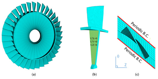
Figure 1.
Finite element model of the considered bladed disk: (a) overall mesh, (b) blade sector, (c) periodic boundaries.

Table 1.
Fluid working parameters of NASA-ROTOR37 blades.
The modal characteristics of the tuned bladed disk are shown in Figure 2. In this case, the bladed disk is a perfect cyclic periodic structure; thus, the modal shapes are also periodic along the circumferential direction [25]. The number of nodal lines along the circumferential direction for a given modal shape is referred to as the nodal diameter index (NDI). Note that NDI also represents the number of periods along the circumferential direction within a modal shape, as shown in Figure 3. Figure 2 is obtained by the following steps. First, we compute several tens of modes with the lowest modal frequencies. Second, we compute the NDI of each mode. This can be done by directly setting the NDI value if one uses the sector model (Figure 1b) with the periodic boundary condition imposed on the wheel (Figure 1c). Alternatively, if a full-scale model is used (Figure 1a), NDI can be obtained by DFT analysis of the distribution of displacement at the same blade location. In this work, we use the first approach based on ANSYS, and the results shown in Figure 3 can be obtained by post-processing. Third, we sort the modes with the same NDI and link all the modes with the lowest natural frequencies from NDI = 0 to NDI = 18. This gives us the first modal family shown in Figure 2. Linking all the modes with the second lowest natural frequencies from NDI = 0 to NDI = 18 yields the second modal family. Likewise, modal families 3, 4, and 5 are obtained, as shown in Figure 2.
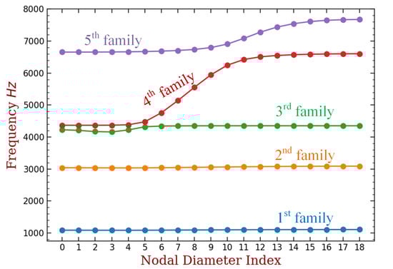
Figure 2.
Natural frequencies of the bladed disk, sorted by nodal diameter index (NDI).
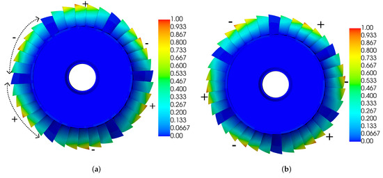
Figure 3.
A pair of double-root modal shapes of the first modal family. The colour represents the absolute value of the overall displacement (to highlight nodal diameters). The areas marked by ‘−’ are out-of-phase with the areas marked by ’+’. (a) NDI = 3, (b) the repeated mode, NDI = 3.
The considered bladed disk has 36 blades. Thus, we can have modes with NDI ranging from 0 (all the blades vibrate in-phase) to 18 (every adjacent blades vibrate out-of-phase), according to the sampling theorem. Except for NDI = 0 and NDI = 18, there is a pair of double-root modes corresponding to each NDI ranging from 1 to 17. Figure 3 shows the pair of double-root modes corresponding to NDI = 3 in the first family. They have the same natural frequencies, and their modal shapes are the same if we rotate Figure 3b by degrees along the clockwise direction. We can roughly understand them as the pair of a sin() and a cos() function with the same frequency in Fourier expansion. The double-root modes are represented by the same point in Figure 2. In summary, the number of modes in a modal family is equal to the number of blades N, and in this paper .
Modes in the same family have similar blade deformation if the frequency-NDI curve is flat, as in the 1st, 2nd, and 3rd families in Figure 2. In this case, we can also deduce that most of the strain energy is on the blades. Otherwise, if a significant proportion of energy is distributed on the disk, when NDI increases, the disk deforms more dramatically, and its strain energy will also increase, thus increasing the natural frequencies. Generally, the modes on the flat part in a frequency-NDI curve are referred to as the ’blade-dominated’ modes. The 1st, 2nd, and 3rd modal families are dominated by the first bending, first torsion, and second bending deformations of the blades, as shown in Figure 4a–c, respectively. The natural frequencies in the 4th family start from the neighbour of the 3rd family to a value very close to the starting of the 5th family. From NDI = 5 to NDI = 10, the frequency significantly increases with NDI; this means that the disk is also involved in the modal vibration. The 4th family presents a typical ‘veering’ phenomenon. We can see that its modal shape is close to the 3rd family at the beginning (Figure 4c,d), and it will finally shift to another type of deformation close to the 5th family (Figure 4e,f). More detailed knowledge of the dynamics of bladed disks can be found in the literature [25,26,27,28].
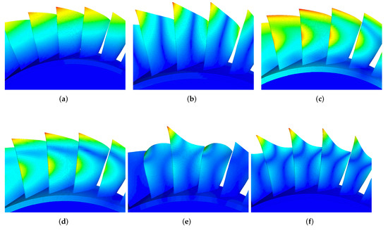
Figure 4.
Blade deformation of different modal families. The colour represents the absolute value of the overall displacement. (a) 1st family, NDI = 2; (b) 2nd family, NDI = 2; (c) 3rd family, NDI = 2; (d) 4th family, NDI = 2; (e) 4th family, NDI = 14; (f) 5th family, NDI = 2.
In this work, we use the aeroelastic stability of the first modal family to illustrate the proposed approaches. Note that the natural frequency is around 1000 Hz because we constrain all the degrees-of-freedom (DOFs) on both sides of the disk surface, as shown in Figure 1b. We intentionally impose this strong boundary condition so that the modes of this family have a similar frequency, because they are all dominated by the blade bending deformation as presented and discussed. Thus, we can use a single fluid field analysis with moving mesh on the blade surface to obtain the required aeroelastic influence coefficients, as will be shown later. The choice of boundary conditions does not change the findings and conclusions of this paper.
In the following, mechanical mistuning with different patterns and levels will be imposed to the bladed disk. The varying of the least modal damping ratio will be used as the performance criterion of the aeroelastic stability enhancement. Our aims are (1) to find an interpretation to quantitatively understand the computed results and (2) to find a way to predict the performance of a mistuning pattern before the full aeroelastic analysis.
2.2. Dynamic Model of the Mistuned Bladed Disk
With the mesh presented in Figure 1, the full dynamic equation of the mistuned bladed disk can be obtained by finite element method, as follows:
where is the displacement vector; , , and are the nominal stiffness, mass, and structural damping matrices, respectively; and are the deviation of stiffness and mass matrices due to mistuning, respectively; is the excitation force vector; and is the aerodynamic force vector. In the analysis of aeroelastic stability, the structural damping and excitation force are neglected, and this gives and .
Because all the modes in the first families have nearly the same frequencies (Figure 3), we can use an approach termed the fundamental model of mistuning (FMM) [29] to reduce the size of the problem. The basic idea is to use all the tuned modal shapes of the targeting family as the reduced basis to express the displacement of the bladed disk, namely:
where N is the overall number of blades and also the number of modes in one modal family; is the reduced displacement vector with only N degrees-of-freedom; and are the (mass normalized) modal shapes from the same family, obtained by the following eigenvalue problem:
In this paper, we assemble matrix by the following order:
where superscripts + and - refer to double-root modes with the same NDI, and subscript refers to the NDI of the modal shape. The order of modes in the columns of does not affect the conclusions, but knowing it is beneficial for interpolating and reproducing the presented results.
Introducing Equation (2) into (1), and left-multiplying both sides of the equation by , the reduced dynamic equation can be obtained:
where , and is the eigenvalue associated with in the solutions of Equation (3). The cyclic periodicity of each (represented by NDI, as illustrated in Figure 2 and Figure 3) is used, and this leads to:
where is the average frequency of the modal family. Matrix is written as follows:
where coefficients for are determined by
where is the frequency deviation of the blade in sector s and . Please refer to the original paper [29] for the detailed derivation.
Note that the for constitute the mistuning pattern. The alternate, pure wave, and random patterns are given by Equations (9), (10), and (11), respectively.
where A, B, C, and D are constants; h is the harmonic index and represents the repetitions of the pattern along the circumference direction; and is the sampling function of the underlying distribution. In this paper, we only investigate one mistuning pattern at one time; we do not investigate their combinations.
Vector represents the fluid force applied on the blades caused by the vibration of blades (). Here, aerodynamic influence coefficient (AIC) [30] is employed to express the aeroelastic force:
where is the aerodynamic influence coefficient matrix, and it contains complex values. AIC represents the aeroelastic force acting on a certain blade, induced by the steady-state deformation of the reference blade (numbered as the 1st blade in this paper), and projected to the same modal coordinate (the first bending mode in this paper). Specifically, the AIC of the jth blade is computed by
where a is the amplitude of the reference blade following modal shape , is the corresponding natural frequency of , is the vector of force amplitude acting on the jth blade generated by the deformation of the reference blade, and is the projection of to modal shape . Note that are are determined by a, , and , but their exact expressions are not yet found. Here, we use the CFD software ANSYS/CFX to compute for a given blade deformation. The moving grid technique is used to introduce the vibration of the reference blade. Only the reference blade is deforming according to the targeted modal shape and frequency. The other blades are not deformed, and their surface pressure will be obtained by CFD analysis. Initially, CFD analysis yields the steady-state time series of pressure acting on blades. Then, we convert the pressure field to nodal force vector by element integration. A DFT analysis is performed on the time series of the force acting on each node, to extract as the amplitude of the harmonic component with frequency . In this way, we can obtain a row of matrix by Equation (13). Due to cyclic symmetry, all the remaining rows of matrix can be generated by shifting the components in the first row. This method is relatively mature and details can be found in the literature [16,30]. For the sake of brevity, we do not dive into details of the technique.
Substituting Equations (5)–(12) leads to a linearized dynamic equation. The free vibration of the bladed disk with aeroelastic coupling can be accessed by the following eigenvalue problem:
where natural frequencies and modal shapes can have complex values, for . Generally, is not symmetric, and the eigenvalues are no longer double roots. The aeroelastic damping ratio of the jth mode can be given by
The system becomes unstable if there are negative values of aerodynamic damping ratio. Therefore, we will use the minimum value of aerodynamic damping ratio among all the modes, denoted by , as an indicator for the aeroelastic stability of the system. Namely,
If , the system is unstable. If increases after some treatment, maybe the value is still negative, but the system is easier to stabilize by material or structural damping, so we can also conclude that the aeroelastic stability is improved.
2.3. Interpretation to the Aerodynamic Damping of the Mistuned Bladed Disk
Normally, one should first solve Equation (14) many times, with a different mistuning pattern each time. Then, the best mistuning pattern can be selected. We have seen in the literature, and will see in the following sections, that some mistuning patterns can lead to a significant improvement of aeroelastic stability, while others cannot. However, this phenomenon cannot be well understood by pure numerical analysis. In this section, we present an interpretation to understand such a performance difference.
First, we obtain the eigensolutions of the tuned bladed disk by solving Equation (14) with , namely:
where is the jth eigenvalue, and is the associated eigenvector. Overall, N linearly independent eigenvectors will be obtained, and they can be used as a basis to express any vectors with N components.
Second, we expand the ith eigenvector of Equation (14) by a linear combination of all the , written as follows:
where is the array of coefficients. In this way, we can have
if eigenvectors are normalized by and . Equation (18) also provides a way to compute the projection coefficients . When the tuned modal basis is known by Equation (17), is then obtained by solving a linear equation with the right-hand side of the given mistuned modal shape . Iterating i from 1 to N, all the mistuned modes can be projected to the space spanned by the tuned modal basis.
Third, let us recall from Equation (14) that and its associated eigenvalue have the following relationship:
Likewise, Equation (17) endows and its associated eigenvalue with the following relationship:
Substituting Equation (18) into (20), and using Equation (21), we can get
where is neglected, as it is much smaller than and .
Eventually, we rewrite Equation (22) into
This equation shows that each mistuned aeroelastic eigenvalue is the linear superposition of all the tuned eigenvalues, and the weight coefficients are determined by projecting the associated mistuned eigenvector (modal shape) to the space spanned by all the tuned eigenvectors (Equation (18)). On this basis, we can further extend the equation to the following levels: (1) interpreting the mechanism of aeroelastic stability enhancement induced by mistuning; and (2) predicting the aeroelastic stability enhancement of a given mistuning pattern.
2.3.1. Level 1: Interpret the Mistuned Aeroelastic Damping
Eigenvalues of the bladed disk are complex numbers when the aeroelastic effect is considered. The aeroelastic damping ratio, as the fraction between the imaginary and real parts of , varies from 0.1% to 3%, as frequently reported in the literature [6,7,16,17]. This means that the imaginary part of is much smaller than the real part. Accordingly, we can find some approximated expressions:
According to Equation (15), the aeroelastic damping can be approximated:
Introducing Equations (15)–(23), we can have a good approximation of the aeroelastic damping ratio associated with :
where
is the aeroelastic damping ratio associated with . Normally, slight mistuning will not introduce significant deviation of natural frequencies; therefore, we can let , and Equation (27) becomes
Equation (29) shows that each mistuned aeroelastic damping is also the linear superposition of all the tuned damping ratios, and the weight coefficients are determined by projecting the associated mistuned eigenvector (modal shape) to the space spanned by all the tuned eigenvectors (Equation (18)). This is the first contribution of this paper.
2.3.2. Level 2: Evaluate a Given Mistuned Pattern
With the method presented in the previous section, the aeroelastic damping ratio of each mode from a mistuned bladed disk can be fully understood by expanding the modal shape (Equation (18)) and superposing the tuned damping ratios according to the expanding weights (Equation (29)). The premise is that we have already obtained the mistuned aeroelastic modes. In this regard, it can only be called an interpretation approach.
It is worthy to investigate whether we can use the mistuned modal shapes without aeroelastic effects to estimate the aeroelastic damping. If applicable, the analysis of bladed disks with mistuning and aeroelastic effects can be done separately. The aeroelastic damping results can come from numerical models with higher accuracy or experiments. Moreover, the full aeroelastic analysis on the mistuned bladed disk is avoided, and the design of mistuning pattern can be accelerated.
To do so, we can first solve the following eigenvalue problem:
where is the ith eigenvalue, and is the associated eigenvector. Overall, N pairs of solutions will be obtained, and each corresponds to a natural frequency and the associated modal shape of the mistuned bladed disk without aeroelastic effects. We can also project into the space spanned by N eigenvectors of Equation (17), which is written as follows:
With unknown, we can use as an approximation to proceed with the derivation from Equations (21) to (29). Eventually, we can use to replace in Equation (29), namely:
This equation provides a way to predict the aeroelastic enhancement of a given mistuning pattern prior to the full aeroelastic analysis. This is the second contribution of this paper. We will discuss its accuracy in the following sections.
3. Results
3.1. Aeroelastic Damping of the Tuned Blade Disk
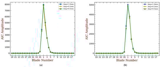
The aeroelastic damping of the tuned blade disk is obtained by solving Equation (17). To do so, matrix , containing the aerodynamic influence coefficients (AICs), should be computed in advance. AICs computed with amplitude mm, mm, and mm are compared in Figure 5, where both conditions shown in Table 1 are computed. Results show that AICs are nearly independent with the amplitude of blade in the computing routine; thus, the linear relationship between the modal displacement and aeroelastic force is verified. The blade with larger distance to the reference (1st) blade has smaller aerodynamic force, and this is expected. Because of the blade torsion, the AICs are not symmetric with respect to blade index 1. For example, the AIC of blade 2 is not equal to that of blade 36. This means that is not a symmetric matrix and the eigenvalues with aeroelastic effects are no longer double roots. In the following analysis, the AICs obtained with modal amplitude 1.0 mm at the unstable working point will be used.
The aerodynamic damping is computed and shown in Figure 6. The modes still have similar frequencies around 1080–1094 Hz, which are also close to the results shown in Figure 2. However, the corresponding aeroelastic damping is significantly different, and unstable modes with negative aeroelastic damping can be found (with NDI 14–21). These observations indicate that matrix does not significantly change the overall stiffness of the system but mainly affects the damping properties. These results also support the assumption we made in Equation (22).
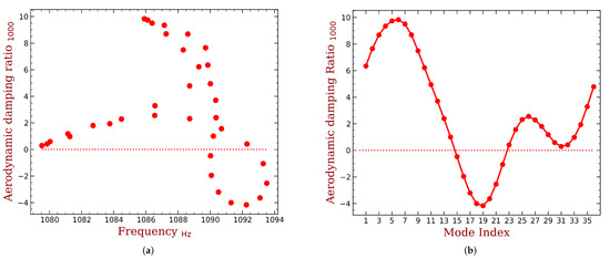
Figure 6.
Aerodynamic damping ratios of the tuned bladed disk. The mapping between the modal index and NDI is shown in Equation (4). (a) Sorted by frequency, (b) sorted by modal index.
3.2. Interpreting the Aeroelastic Damping of Mistuned Bladed Disk
With the results presented in the previous section, we can now use the proposed method to understand the aeroelastic damping of a mistuned blade disk. First, let us consider mistuning of the wave and alternate patterns. Note that the alternate pattern is equivalent to the wave pattern with , as illustrated in Figure 7.
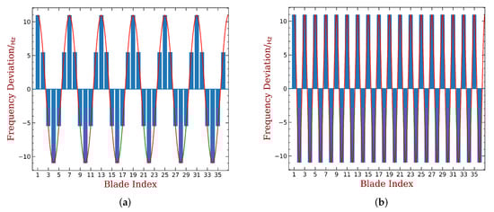
Figure 7.
Illustration of some mistuning patterns. (a) Wave with h = 6, (b) alternate, also wave with h = 18.
The results of the h = 6 wave pattern are shown in Figure 8a, where two groups of data are compared. The first group is the data directly obtained by solving the full aeroelastic problem shown in Equation (14). The other group of results (labelled ’Appro Data’) is obtained by (1) expanding the modal shapes with Equation (18), and (2) reconstructing the damping ratio by superposing the tuned results according to Equation (29). These two groups of results are very close to each other, verifying the correctness of the derivations shown in Section 2.3. Compared with Figure 6b, the least aeroelastic damping has been improved from around −0.4% to −0.2%. This can be interpreted by expanding the least damped mode into the tuned modal space, as shown in Figure 8b. The least damped mode is mainly contributed by the tuned mode with NDI = 19, whose aeroelastic damping ratio is around −0.4%. However, the mistuned mode also has contributions from modes with NDI 13 (damping ratio 0%) and 25 (damping ratio 0.2%). Their contributions eventually improve the damping of the mistuned mode.
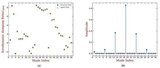
Figure 8.
Interpreting the aeroelastic damping with h = 6 wave mistuning. The mistuning modes are sorted by natural frequencies in ascending order. The mapping between the tuned modal index and NDI is shown in Equation (4). (a) Damping ratio reconstructed by Equation (29), (b) the weight of tuned modes to the least damping mistuning mode.
Results of the alternate pattern are shown in Figure 9, organized in the same way as Figure 8. Good agreements can also be observed in Figure 9a. Figure 9b indicates that the least damped mode now has the secondary contribution from tuned mode with NDI = 1, whose damping ratio is 0.6% (Figure 6b). Thus, the least aeroelastic damping is improved further.
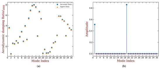
Figure 9.
Interpreting the aeroelastic damping with alternate (also h = 18 wave) mistuning. The mistuning modes are sorted by natural frequencies in ascending order. The mapping between the tuned modal index and NDI is shown in Equation (4). (a) Damping ratio reconstructed by Equation (29), (b) the weight of tuned modes to the least damping mistuning mode.
Figure 10 summarizes the least aeroelastic damping ratio of wave patterns with all the h values. Once again, good agreements are observed. This verifies that the proposed method is applicable for the wave and alternate patterns.
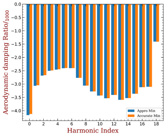
Figure 10.
Reconstructing the least aeroelastic damping with wave mistuning, from h = 0 to h = 18.
Let us continue to verify the proposed approach with the random pattern. The results are summarized in Figure 11, where random mistunings with standard deviations of 0.3%, 0.5%, and 0.8% are considered. For each case, 1000 samples are generated from uniform distribution with zero mean and the given standard deviation. For each sample, we extract its least aeroelastic damping by two means. One is the data directly obtained by solving the full aeroelastic problem shown in Equation (14). The other data (labeled ’Appro Data’) is obtained by (1) expanding the modal shapes with Equation (18), and (2) reconstructing the damping ratio by superposing the tuned results according to Equation (29). Eventually, we divide the results into 40 intervals and count their appearance frequency. We also choose 30 out of 1000 samples to provide point-to-point comparisons, as shown in Figure 12. Good agreements can be observed in both figures. This verifies that the proposed method is also applicable for the random (arbitrary) patterns. We can further understand the samples with higher aeroelastic stability by the same method presented in Figure 8b and Figure 9b. It can also be confirmed that a higher aeroelastic damping is always associated with more contributions of the tuned modes with higher damping ratio. For the sake of brevity, these results for the random mistuning are omitted.
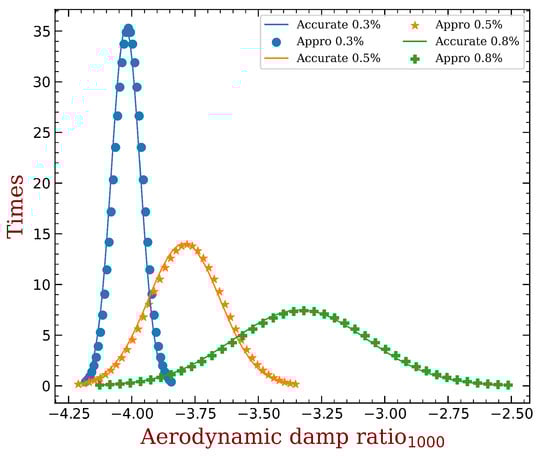
Figure 11.
Reconstructing the frequency graph of aeroelastic damping with random mistuning, with standard deviation 0.3%, 0.5%, and 0.8%. Each time, 1000 samples are computed.
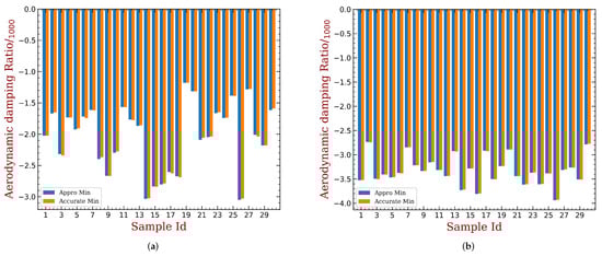
Figure 12.
Reconstructing the least aeroelastic damping with random mistuning, with 30 of 1000 samples shown for each case. (a) Standard deviation 0.2%, (b) standard deviation 0.8%.
3.3. Predicting the Aeroelastic Enhancement of a Given Mistuning Pattern
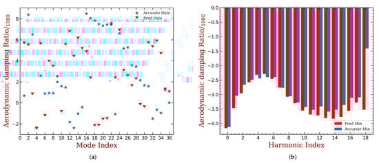
As presented in Section 2.3.2, we can also use Equations (31) and (32) to predict the enhancement of aeroelastic stability of a given mistuning pattern. Figure 13a compares the predicted results with the accurate data, showing a dramatic point-to-point difference. This is due to the approximation made in Equation 32, by replacing the damped eigenvector by the undamped one. However, the least damping ratio is well predicted, and this is the critical performance indicator of a mistuning pattern. We compare the predicted least damping ratios of the wave pattern with h = 1 to h = 18 (alternate pattern) with the accurate data in Figure 13b. Despite a minor error, good agreements can be found in the overall trend from h = 1 to h = 17. This means that the correlation in terms of the least damping ratio found in Figure 13a is not a coincidence. The prediction fails only for the alternate mistuning (h = 18), which has the best performance in our investigation. This is not to say that we failed to find the ’final’ answer to designing an intentionally mistuned bladed disk. On one hand, mistuning can improve the aeroelastic damping. On the other hand, it may lead to severe vibration amplification. In this regard, the designer should also conduct analysis on the forced response, and make a compromised decision for the final mistuning pattern. At this level, the designer needs to know the least aeroelastic damping of each mistuning pattern, and this can be well predicted by the proposed method with ease.
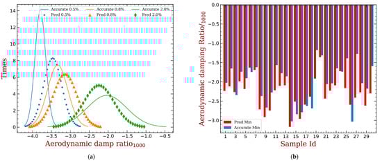
We also consider random mistuning and conduct statistical analysis. Figure 14a compares the frequency graphs of the predicted results with the accurate data, at several standard deviation levels, each with 20,000 samples. At lower mistuning strength, the predicted data has significant error, but this error is reduced when mistuning strength becomes higher. In addition, Equations (31) and (32) fail to provide a point-to-point prediction, as shown in Figure 14b. At the design phase, it is more important to know the mathematical expectation, namely the mean value of each frequency graph. In this regard, the predicted results have satisfying accuracy and constitute useful references to the designers.
4. Discussion
With the results presented from Figure 8 to Figure 11, the accuracy of Equations (18) and (29), which underlie the proposed interpretation approach, is validated. Here, we provide some further remarks. Let us recall that the sum of is constrained to 1, as shown in (19). Therefore, we can have the following interpolations concerning the mechanism of aeroelastic stability enhancement induced by mistuning:
- Mistuning cannot increase and would rather decrease the largest aeroelastic damping ratio. It can be demonstrated that if the kth tuned mode has the largest aeroelastic damping ratio. This happens only when and . It is unlikely to perfectly satisfy this condition if mistuning is presented. However, when the mistuning strength is slight, it is more likely to have mistuned modal shapes dominated by the kth tuned mode, namely . In this case, the difference between and is minor. However, with the increase of mistuning strength, the mistuned modes tend to have a more significant contribution from multiple tuned modes. In this case, the difference between and will also be enlarged.
- Mistuning cannot further decrease the smallest aeroelastic damping ratio; thus, it is always beneficial to the aeroelastic stability. It can be demonstrated that if the lth tuned mode has the smallest aeroelastic damping ratio. This happens only when and . As noted earlier, will always be larger than with the presence of mistuning, and this gap is enlarged by the increase of mistuning strength. This remark is illustrated by comparing Figure 8a and Figure 9a with Figure 6b.
- A mistuned mode has higher aeroelastic damping ratio than another, only if its modal has more contribution from the tuned modes with higher aeroelastic damping ratio. The best mistuning pattern is the one who tends to produce modal shapes constructed by the tuned modes with relatively high aeroelastic damping ratio. This remark is illustrated by comparing Figure 8b and Figure 9b with Figure 6b.
Such trends are also frequently reported in the literature [14,15,16,18,31] by numerical analysis. Now, we can confirm that they are general.
5. Conclusions
- (1)
- The aeroelastic damping ratio of a mode in the mistuned bladed disk can be interpreted as follows: it is determined by the contribution of each tuned mode in the associated modal shape. Derivations are given in detail, and the accuracy is validated by numerical investigation. The proposed interpretation is applicable for various mistuning patterns, including the alternate, wave, and random patterns.
- (2)
- Several general conclusions are drawn, confirming the frequently reported trends in the literature [14,15,16,18,31]. First, mistuning cannot increase and would rather decrease the largest aeroelastic damping ratio. Second, mistuning cannot further decrease the smallest aeroelastic damping ratio; thus, it is always beneficial to the aeroelastic stability. Third, a mistuned mode has higher aeroelastic damping ratio than another only if its modal has more contribution from the tuned modes with higher aeroelastic damping ratio.
- (3)
- A prediction method is also proposed, providing an acceptable approximation of the least aeroelastic damping of a given mistuning pattern. This is done with the mistuning and aeroelastic effects analyzed separately. The advantages are two-fold. First, the design of mistuning pattern is accelerated. Second, this allows one to introduce more accurate data or models of aeroelastic damping.
Author Contributions
Conceptualization, Y.F. and L.L.; methodology, X.L. and X.Y.; validation, X.L. and Y.F.; writing—original draft preparation, X.L.; writing—review and editing, Y.F.; supervision, L.L.; funding acquisition, Y.F. and L.L. All authors have read and agreed to the published version of the manuscript.
Funding
This work was funded by Major Projects of Aero-Engines and Gas Turbines (2017-IV-0002-0039 and J2019-IV-0023-0091), Aeronautical Science Foundation of China (2019ZB051002), and Advanced Jet Propulsion Creativity Center (Projects HKCX2020-02-013 and HKCX2020-02-016).
Institutional Review Board Statement
Not applicable.
Informed Consent Statement
Not applicable.
Data Availability Statement
The data presented in this study is available on request from the corresponding author.
Conflicts of Interest
The authors declare no conflict of interest. The funders had no role in the design of the study; in the collection, analyses, or interpretation of data; in the writing of the manuscript, or in the decision to publish the results.
References
- Srinivasan, A.V. Flutter and Resonant Vibration Characteristics of Engine Blades: An IGTI Scholar Paper. In Proceedings of the ASME 1997 International Gas Turbine and Aeroengine Congress and Exhibition, Orlando, FL, USA, 2–5 June 1997. [Google Scholar] [CrossRef]
- Whitehead, D.S. Effect of Mistuning on the Vibration of Turbo-Machine Blades Induced by Wakes. J. Mech. Eng. Sci. 1966, 8, 15–21. [Google Scholar] [CrossRef]
- Bendiksen, O.O. Flutter of mistimed turbomachinery rotors. J. Eng. Gas Turbines Power 1984, 106, 25–33. [Google Scholar] [CrossRef]
- Groth, P.; Mårtensson, H.; Andersson, C. Design and Experimental Verification of Mistuning of a Supersonic Turbine Blisk. J. Turbomach. 2010, 132, 011012. [Google Scholar] [CrossRef]
- Figaschewsky, F.; Kuhhorn, A.; Beirow, B.; Nipkau, J.; Giersch, T.; Power, B. Design and analysis of an intentional mistuning experiment reducing flutter susceptibility and minimizing forced response of a jet engine fan. In Proceedings of the ASME Turbo Expo 2017: Turbomachinery Technical Conference and Exposition, Charlotte, NC, USA, 26–30 June 2017; Volume 7B-2017, pp. 1–13. [Google Scholar] [CrossRef]
- Biagiotti, S.; Pinelli, L.; Poli, F.; Vanti, F.; Pacciani, R. Numerical Study of Flutter Stabilization in Low Pressure Turbine Rotor with Intentional Mistuning. Energy Procedia 2018, 148, 98–105. [Google Scholar] [CrossRef]
- Corral, R.; Khemiri, O.; Martel, C. Design of mistuning patterns to control the vibration amplitude of unstable rotor blades. Aerosp. Sci. Technol. 2018, 80, 20–28. [Google Scholar] [CrossRef]
- Kaza, K.R.V.; Kielb, R.E. Flutter and response of a mistuned cascade in incompressible flow. AIAA J. 1982, 20, 1120–1127. [Google Scholar] [CrossRef]
- Kielb, R.E.; Kaza, K.R.V. Aeroelastic Characteristics of a Cascade of Mistuned Blades in Subsonic and Supersonic Flows. J. Vib. Acoust. 1983, 105, 425–433. [Google Scholar] [CrossRef]
- Kielb, R.E.; Kaza, K.R.V. Effects of Structural Coupling on Mistuned Cascade Flutter and Response. J. Eng. Gas Turbines Power 1984, 106, 17–24. [Google Scholar] [CrossRef]
- Crawley, E.F.; Hall, K.C. Optimization and Mechanisms of Mistuning in Cascades. J. Eng. Gas Turbines Power 1985, 107, 418–426. [Google Scholar] [CrossRef]
- Shapiro, B. Symmetry approach to extension of flutter boundaries via mistuning. J. Propuls. Power 1998, 14, 354–366. [Google Scholar] [CrossRef][Green Version]
- Kielb, R.E.; Hall, K.C.; Hong, E.; Pai, S.S. Probabilistic Flutter Analysis of a Mistuned Bladed Disks. In Proceedings of the ASME Turbo Expo 2006: Power for Land, Sea, and Air, Barcelona, Spain, 8–11 May 2006; pp. 1145–1150. [Google Scholar] [CrossRef]
- Li, L.; Yu, X.; Wang, P. Research on aerodynamic damping of bladed disk with random mistuning. In Proceedings of the ASME Turbo Expo 2017: Turbomachinery Technical Conference and Exposition, Charlotte, NC, USA, 26–30 June 2017; Volume 7B-2017, p. V07BT36A010. [Google Scholar] [CrossRef]
- Liu, X.; Li, L.; Fan, Y.; Deng, P. Improving the Aero-Elastic Stability of Bladed Disks through Parallel Piezoelectric Network. In Proceedings of the 2018 Joint Propulsion Conference, Cincinnati, OH, USA, 9–11 July 2018. [Google Scholar] [CrossRef]
- Zhang, X.; Wang, Y. Mistuning Effects on Aero-elastic Stability of Contra-Rotating Turbine Blades. Int. J. Aeronaut. Space Sci. 2019, 20, 100–113. [Google Scholar] [CrossRef]
- Fang, M.; Wang, Y. Intentional Mistuning Effect on the Blisk Vibration with Aerodynamic Damping. AIAA J. 2022, 1–10. [Google Scholar] [CrossRef]
- Liu, X.; Fan, Y.; Li, L.; Yu, X. Improving Aeroelastic Stability of Bladed Disks with Topologically Optimized Piezoelectric Materials and Intentionally Mistuned Shunt Capacitance. Materials 2022, 15, 1309. [Google Scholar] [CrossRef] [PubMed]
- Martel, C.; Corral, R.; Llorens, J.M. Stability Increase of Aerodynamically Unstable Rotors Using Intentional Mistuning. J. Turbomach. 2008, 130, 011006. [Google Scholar] [CrossRef]
- Bleeg, J.M.; Yang, M.T.; Eley, J.A. Aeroelastic Analysis of Rotors With Flexible Disks and Alternate Blade Mistuning. J. Turbomach. 2009, 131, 1–9. [Google Scholar] [CrossRef]
- Martel, C.; Sánchez, J.J. Intentional Mistuning with Predominant Aerodynamic Effects. In Proceedings of the ASME Turbo Expo 2018: Turbomachinery Technical Conference and Exposition, Oslo, Norway, 11–15 June 2018; Volume 7C, pp. 1–11. [Google Scholar] [CrossRef]
- Hsu, K.; Hoyniak, D. A fast influence coefficient method for aerodynamically mistuned disks aeroelasticity analysis. J. Eng. Gas Turbines Power 2011, 133, 1–10. [Google Scholar] [CrossRef]
- Panovsky, J.; Kielb, R.E. A design method to prevent low pressure turbine blade flutter. In Proceedings of the ASME 1998 International Gas Turbine and Aeroengine Congress and Exhibition, Stockholm, Sweden, 2–5 June 1998; Volume 5. [Google Scholar] [CrossRef]
- Campobasso, M.S.; Giles, M.B. Analysis of The Effect of Mistuning on Turbomachinery Aeroelasticity. In Proceedings of the 9th International Symposium on Unsteady Aerodynamics, Aeroacoustics and Aeroelasticity of Turbomachines, Lyon, France, 4–8 September 2000; pp. 885–896. [Google Scholar]
- Ewins, D.J. Vibration Modes of Mistuned Bladed Disks. J. Eng. Power 1976, 98, 349–355. [Google Scholar] [CrossRef]
- Slater, J.C.; Minkiewicz, G.R.; Blair, A.J. Forced Response of Bladed Disk Assemblies—A Survey. Shock Vib. Dig. 1999, 31, 17–24. [Google Scholar] [CrossRef]
- Castanier, M.P.; Pierre, C. Modeling and Analysis of Mistuned Bladed Disk Vibration: Current Status and Emerging Directions. J. Propuls. Power 2006, 22, 384–396. [Google Scholar] [CrossRef]
- Srinivasan, A.V. Vibrations of Bladed-Disk Assemblies—A Selected Survey (Survey Paper). J. Vib. Acoust. 1984, 106, 165–168. [Google Scholar] [CrossRef]
- Feiner, D.M.; Griffin, J.H. A Fundamental Model of Mistuning for a Single Family of Modes. J. Turbomach. 2002, 124, 597. [Google Scholar] [CrossRef]
- Hanamura, Y.; Tanaka, H.; Yamaguchi, K. A Simplified Method to Measure Unsteady Forces Acting on the Vibrating Blades in Cascade. Bull. JSME 1980, 23, 880–887. [Google Scholar] [CrossRef]
- Fu, Z.; Wang, Y. Aeroelastic Analysis of a Transonic Fan Blade with Low Hub-to-Tip Ratio including Mistuning Effects. J. Power Energy Eng. 2015, 3, 362–372. [Google Scholar] [CrossRef]


Publisher’s Note: MDPI stays neutral with regard to jurisdictional claims in published maps and institutional affiliations. |
© 2022 by the authors. Licensee MDPI, Basel, Switzerland. This article is an open access article distributed under the terms and conditions of the Creative Commons Attribution (CC BY) license (https://creativecommons.org/licenses/by/4.0/).