Observer-Based Backstepping Adaptive Force Control of Electro-Mechanical Actuator with Improved LuGre Friction Model

Abstract

A dynamic load simulator, which can reproduce on-ground aerodynamic hinge moment of control surface, is an essential rig for the performance and stability test of an aircraft actuation system. In this paper, an observer-based backstepping adaptive control (OBAC) strategy with an improved friction model is proposed to deal with the force tracking problem of an electro-mechanical actuator under the influence of nonlinear friction and lumped disturbances. First, The LuGre friction model is improved by introducing the load effect of electrical linear load simulator (ELLS), and both dynamic and static parameters are identified with experimental data. Then, the ELLS system is divided into a loading subsystem and actuation subsystem for backstepping controller deign. The estimation of the position disturbance is obtained using an extended state observer and used for feedforward compensation for the loading subsystem. To reject the disturbance of friction parameter uncertainties for actuation subsystem, a friction scale factor with a reasonable adaptive updating law is introduced during the friction compensation process. Finally, the stability of the whole closed-loop system is demonstrated using a Lyapunov-based method, and experiments are performed to validate the effectiveness of the developed algorithm.

1. Introduction

With the development of power-by-wire (PBW) technology in aerospace field, the flight actuation system is gradually replaced from hydraulic power to the electrical [1,2]. The electro-mechanical actuator, which belongs to one of the PBW actuator and is capable of direct conducting the transform from electric to mechanical power, is advantageous for power management, integration and maintenance [2]. Currently, EMAs have come to service in the partial systems of civil and military aircrafts, including ram air inlet system, B787 wheel brake, A350 horizontal stabilizer, etc. [1,3,4].

A great deal of work related to laboratory tests as well as flight tests of EMA has been conducted to establish the credibility of electric actuation for primary or crucial aircraft system. NASA conducted the flight test of the EMA performance on the F-18 aileron for the comparison with the origin hydraulic actuator [5]. At the Covadis project, the researchers succeeded in introducing EMA for a flight test on an aileron of A320, where a series of ground tests were finished in advance on an iron bird test bench [6]. The laboratory or flight tests of EMA for landing gear, spoiler, etc. have already made progress [7,8].

Qualification of EMAs relying on pure fight test is a high-cost, high-risk and time-consuming process. Therefore, it is essential to develop an on-ground load simulator to verify the performance of the PBW actuator [9,10]. This is an effective way to foresee and detect the potential problems of the whole actuation system. Due to the development of high-performance power electronics, motors and mechanical transmission, electro-mechanical actuators are suitable for low-power position control applications and cover different domains [11,12].

The utilization of an electro-mechanical actuator as a dynamic load generator, which is normally known as an electric linear load simulator (ELLS), has gradually received increasing attention. Compared to the widely used electro-hydraulic load simulators, electro-mechanical actuators are advantageous for durability, reliability and suitable application on light load simulators [12].

ELLS is generally expected to provide loading force for tested actuator by tracking the command signal. Its loading accuracy is mainly influenced by the external position disturbance and internal nonlinear friction [13]. Research on how to eliminate these influences and improve the dynamic loading performance has attracted increasing attentions. For ELLS, the active motion from tested actuator causes strong position disturbance, which can seriously reduce the tracking accuracy.

To reject this external disturbance, structure invariance compensation approach based on speed feedforward compensation is widely utilized and recognized as one of the most effective methods [14]. Additionally, in the situations of low speed or frequently varied speed directions, the friction nonlinearity may cause dead zone, creep and large steady state error [15,16]. Its negative effect is more apparent for ELLS, which is usually applied for simulating light loads. The relevant research can be divided into two categories: model-based and model-free friction compensation strategies, and the former is based on various friction models.

Kang et al. conducted friction modelling and identification based on GMS friction model and designed an adaptive terminal sliding model force control strategy by estimating the disturbance boundary [3]. Yao et al. proposed a robust LuGre-model-based friction compensation strategy in which the unmeasurable state is estimated by a dual state observer for a hydraulic load simulator [17].

Alleyne et al. adopted a novel friction model by combining the Karnopp and Stribeck friction models and designed an adaptive controller to eliminate the friction influence for hydraulic load simulator [18]. Wang et al. used the hyperbolic tangent function to describe the stick-slip friction phenomenon in the backstepping controller development process [19]. The obvious advantage is to successfully obtain the differential calculation of the virtual control, whereas this friction model cannot sufficiently consider the friction variations in the pre-slip stage.

The model-based friction compensation approach generally includes parameter identification, which requires abundant post-experiment data and complex optimization algorithm. In addition, the option of different friction models and parameter identification accuracy seriously impact the effective of proposed controller. Therefore, some researchers focus on the model-free method, the overall consideration of which is to treat the friction nonlinearity as unknown disturbance. Wang et al. designed a proportional resonant controller for electric torque load simulator based on Nyquist diagram and adopted phase angle compensation technology to optimize the bandwidth [20].

Zhao et al. developed a feedforward inverse model controller to enhance the load bandwidth without destroying the stability, the key of which is to solve the inverse model of the system transfer function [21]. Jing et al. designed dual extended state observers to estimate the friction and position disturbances for compensation for hydraulic load simulator [22]. Other robust control approaches, including quantality feedback theory control [23], intelligent control [24,25] and H-Infinity control [26], have been used for load simulator.

With above overall investigations, the model-based control approach is more attractive on its less complexity and convenience for engineering practice. At the pre-slip stage, a minor displacement occurs due to approximate elastic deformation [27]. The load amplitude may show significant influence on friction. However, the mainly dependent friction model, such as Stribeck model or traditional LuGre model [27], cannot evaluate these factors simultaneously. Therefore, an improved friction model will be proposed and used for friction compensation. Considering the position disturbance, parameter uncertainties and unknown disturbance for ELLS, the extended state observer and adaptive control law will be simultaneously utilized to achieve high accuracy and strong robustness.

The rest of this article is organized as follows: Section 2 presents the system description and mathematical model of ELLS. Then, in Section 3, an improved LuGre based friction model is established and the friction parameters are identified. Section 4, an observer-based backstepping adaptive control strategy is proposed to achieve high dynamic tracking performance. Section 5 conducts the experiment validation to prove the effective of the propose control algorithm. Finally, conclusions summarize the main contributions of this study.

2. System Description and Mathematical Model

The concerned object in this paper is shown in Figure 1. The left side is the electro-mechanical actuator under test, whereas the right side is another electro-mechanical actuator functioning as the ELLS. The servo drive modulus accepts the control output signal from controller and drive the motor. The linear force is transformed from the motor torque the via the screw-nut mechanism and applied on the tested actuator. In normal operation, the actuator under test is responsible for active motion by tracking the desired position command. For the ELLS, the same time as the servo loading is conducted, a passive pursuit movement is required along with tested actuator.

The torque equilibrium and force equilibrium functions are, respectively, expressed as:

$$T_{\mathrm{m}}=J_{\mathrm{m}}\frac{\mathrm{d}{\omega }_{\mathrm{m}}}{\mathrm{d}t}+T_{\mathrm{fm}}+T_{\mathrm{Le}}$$

(1)

$$F_{\mathrm{e}}=M_{\mathrm{e}}{\ddot{x}}_{\mathrm{e}}+F_{\mathrm{f}}+F_{\mathrm{L}}$$

(2)

where T_m is the motor output torque, T_Le is the load torque for motor, J_m is the inertia of motor, ω_m is the motor shaft angular velocity, F_e is the driving force of screw-nut mechanism, F_L is the loading force, M_e is the translational mass of ELLS, x_e is the translational displacement of ELLS, and T_Le and F_f are frictions inside the motor and screw-nut mechanism, respectively.

Considering an ideal screw-nut mechanism with lead l_s, which converts the rotary motion into linear movement:

$${\theta }_{\mathrm{m}}=k_{\mathrm{s}}{x}_{\mathrm{e}}, {\omega }_{\mathrm{m}}={\dot{\theta }}_{\mathrm{m}}=k_{\mathrm{s}}{\dot{x}}_{\mathrm{e}}, F_{\mathrm{e}}=k_{\mathrm{s}}{T}_{\mathrm{Le}}$$

(3)

where k_s = (2π)/l_s is defined as the transform coefficient of screw-nut mechanism.

Remark 1.

The maximum desired loading frequency are generally within 10 Hz, whereas the current loop natural frequency tuned inside motor servo drive can be up to 500 Hz. Therefore, the current loop can be represented as pure gain element:

$$T_{\mathrm{m}}=k_{\mathrm{t}}i\approx k_{\mathrm{t}}{i}_{\mathrm{ref}}$$

(4)

where i and i_ref are actual motor current and current command; k_t is the torque constant.

The force senor is used for loading force measurement, and its deformation is theoretically linear with the force amplitude:

$$F_{\mathrm{L}}=k_{\mathrm{p}}(x_{\mathrm{e}}-x_{\mathrm{p}})$$

(5)

where k_p is the stiffness coefficient of the force sensor, and x_p is the translational displacement of the actuator under test.

Combining Equation (1) to Equation (5), the space-state description of ELLS is:

$$\{\begin{array}{l}{\dot{x}}_1=\frac{k_{\mathrm{p}}}{k_{\mathrm{s}}}{x}_2-k_{\mathrm{p}}{\dot{x}}_{\mathrm{p}}+d_0\\ {\dot{x}}_2=\frac{k_{\mathrm{t}}}{J}u-\frac{T_{\mathrm{f}}}{J}-\frac{x_1}{J{k}_{\mathrm{s}}}\\ {\left[x_1 x_2\right]}^{\mathrm{T}}={\left[F_{\mathrm{L}} {\omega }_{\mathrm{m}}\right]}^{\mathrm{T}}, u=i_{\mathrm{ref}}\end{array}$$

(6)

where $J=J_{\mathrm{m}}+M_{\mathrm{e}}/k_{\mathrm{s}}^2$ is the ELLS total equivalent inertia, $T_{\mathrm{f}}=T_{\mathrm{fm}}+F_{\mathrm{f}}/k_{\mathrm{s}}$ is the lumped friction of ELLS. d₀ represents the parameter uncertainties and unknown disturbances, which are temporarily neglected in above mathematical modelling process for ELLS. ${\dot{x}}_{\mathrm{p}}$ is the position disturbance from tested actuator for ELLS.

From Equation (6), the active motion of tested actuator leads to strong position disturbance. Additionally, there exists nonlinearities in ELLS, including friction and parameters uncertainties. The design goal of control strategy is to achieve high dynamic performance tracking of the loading force, when the loaded electro-mechanical actuator is subjected to these disturbances.

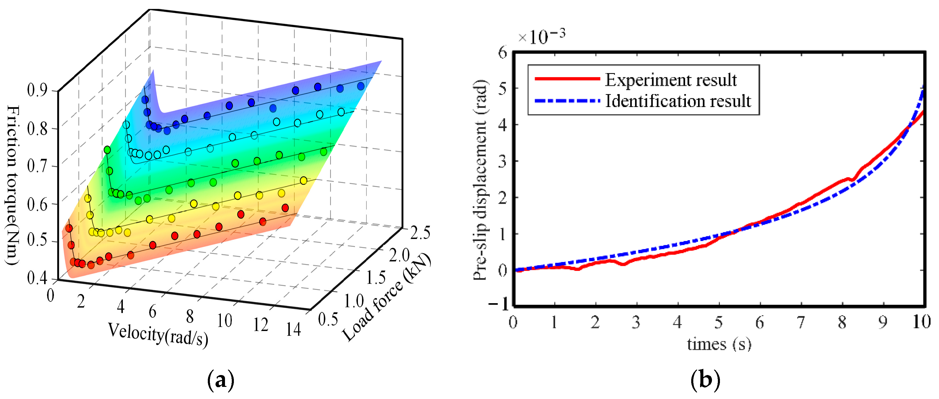
3. Friction Model Improvement and Parameter Identification

To adopt the model-based method to compensate the friction T_f, the widely used LuGre friction model is referred for subsequent work [27]:

$$\{\begin{array}{l}{T}_{\mathrm{f}}={\sigma }_{0}z+{\sigma }_1\frac{\mathrm{d}z}{\mathrm{d}t}+{\sigma }_2{\omega }_{\mathrm{m}}\\ \frac{\mathrm{d}z}{\mathrm{d}t}={\omega }_{\mathrm{m}}-\frac{{\sigma }_0\left|{\omega }_{\mathrm{m}}\right|}{g({\omega }_{\mathrm{m}})}z\\ g({\omega }_{\mathrm{m}})=T_{\mathrm{c}}+(T_{\mathrm{s}}-T_{\mathrm{c}})e^{-{\left({\omega }_{\mathrm{m}}/{\omega }_{\mathrm{st}}\right)}^2}\end{array}$$

(7)

where z is the average deformation of bristles; σ₀ and σ₁ are, respectively, the coefficients of stiffness and damping; σ₂ is the viscous friction coefficient; g(ω_m) represents the Stribeck effect; T_c is the coulomb friction; T_s is the maximum static friction; and ω_st is the Stribeck angular velocity constant.

Unlike traditional hydraulic load mechanism, the loading force is transmitted by screw-nut mechanism for ELLS. The variation of loading force magnitude will directly influence the normal load between the contact surfaces inside screw-nut mechanism, which lead to the approximately linear change of coulomb friction torque and maximum static friction torque [28]. The following functions can be used to describe this relationship:

$$\{\begin{array}{l}{T}_{\mathrm{c}}=a_{\mathrm{c}}\left|F_{\mathrm{L}}\right|+b_{\mathrm{c}}\\ T_{\mathrm{s}}=a_{\mathrm{s}}\left|F_{\mathrm{L}}\right|+b_{\mathrm{s}}\end{array}$$

(8)

where a_s and a_c are the respective gradients of static and coulomb friction torques with respect to load force. b_c and b_s are the respective static and coulomb friction torques on unload occasion.

Substituting Equation (8) into Equation (7), the improved LuGre model considering load effect is:

$$\{\begin{array}{l}{T}_{\mathrm{f}}={\sigma }_{0}z+{\sigma }_1\frac{\mathrm{d}z}{\mathrm{d}t}+{\sigma }_2{\omega }_{\mathrm{m}}\\ \frac{\mathrm{d}z}{\mathrm{d}t}={\omega }_{\mathrm{m}}-\frac{{\sigma }_0\left|{\omega }_{\mathrm{m}}\right|}{g({\omega }_{\mathrm{m}},F_{\mathrm{L}})}z\\ g({\omega }_{\mathrm{m}},F_{\mathrm{L}})=a_{\mathrm{c}}\left|F_{\mathrm{L}}\right|+b_{\mathrm{c}}+\left[(a_{\mathrm{s}}-a_{\mathrm{c}})\left|F_{\mathrm{L}}\right|+b_{\mathrm{s}}-b_{\mathrm{c}}\right]e^{-{\left({\omega }_{\mathrm{m}}/{\omega }_{\mathrm{st}}\right)}^2}\end{array}$$

(9)

where [a_c, b_c, a_s, b_s, ω_st, σ₂] and [σ₀, σ₁] are the static and dynamic parameters vectors, respectively. The differential evolution algorithm will be used for parameter identification, the algorithm implementation process of which was detailed described in our previous contribution [29].

The identification of static friction parameter is based on experimental results under a series of speed and loading force. The actuator under test is commanded to move with steady speed bidirectionally. The ELLS is controlled to follow the active motion and apply constant load force at the same time. To more precisely catch the Stribeck curve of ELLS friction torque, the speed command is more densely distributed at the low speed region.

When the tested actuator moves with different direction, the loading force will present different load performances, i.e., aiding or opposing. Therefore, the friction parameters may be dependent on the operation quarters in identification process. Taking position direction motion as example, the expected static parameter vector is defined as I_p = [a_c⁺, b_c⁺, a_s⁺, b_s⁺, σ₂⁺, ω_st⁺]. With the static parameters identification results, a three-dimensional surface involving friction torque, speed and load force based on the improved LuGre model can be drawn in Figure 2a.

The fitting surface shows good agreement with the actual test data. The intersection between a determined load force cross-section and this surface becomes Stribeck curve, while the intersection between a given velocity cross-section and the surface demonstrates that the friction torque shows an approximately linear relationship with the load force. Similarly, the static parameters identification results in the negative direction can be obtained.

The dynamic parameters are mainly relevant with the immeasurable internal state z at the pre-slip stage. The open-loop experiments are carried out with very slow ramp input current under no-load condition to enhance the effects of dynamic parameters. The expected dynamic parameter vector is defined as I_d = [σ_0,σ₁], and the static friction parameters, which have been already available from previous identification, will be applied for dynamic parameters identification. In Figure 2b, the identification result of pre-slip displacement with identified dynamic and static parameters shows great consistence with the experiment result.

It is noted that the identification process, which has been detailed addressed in literature [30], will not be repeated here. The identification results of both static and dynamic parameters are collected in

Table 1. Parameter identification results of the improved friction model.

	Static Parameters						Dynamic Parameters
	ac (N·m/N)	bc (N·m)	as (N·m/N)	bs (N·m)	σ2 (N·m·s/rad)	ωst (rad/s)	σ0 (N·m/rad)	σ1 (N·m·s/rad)
P.D.	1.01 × 10−4	0.3317	1.13 × 10−4	0.5189	0.0173	0.3468	351.03	0.9014
N.D.	1.07 × 10−4	0.2755	1.46 × 10−4	0.5006	0.0234	0.3431

P.D.: positive direction; N.D.: negative direction.

.

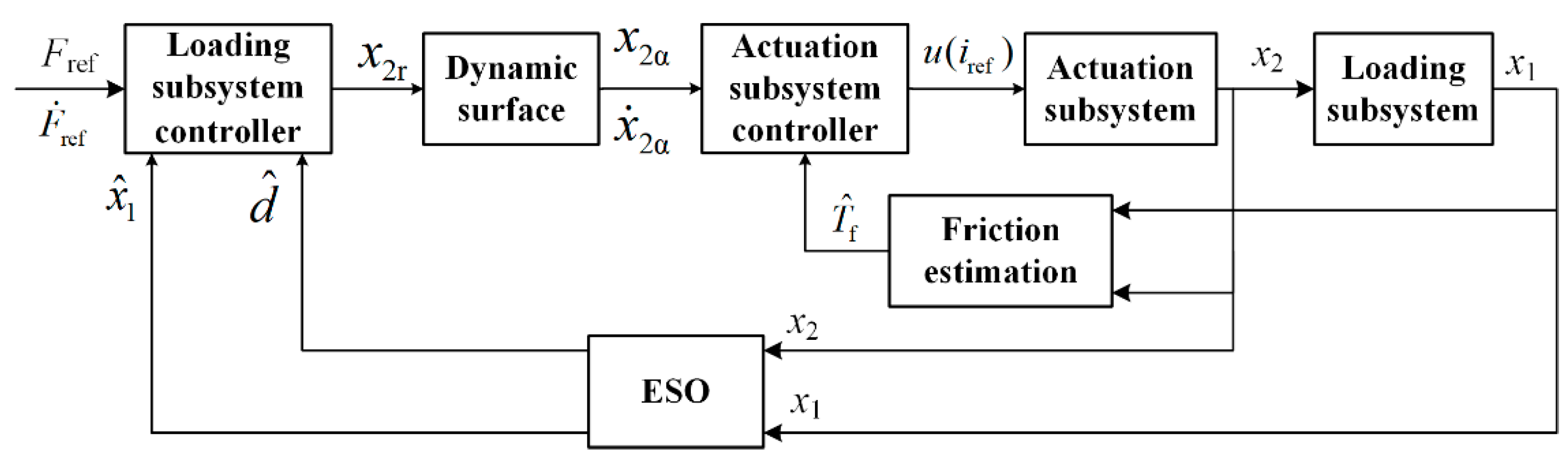
4. Observer-Based Adaptive Backstepping Control

The architecture of the proposed observer-based adaptive backstepping controller is shown in Figure 3. Considering the state functions in Equation (6) and based on the backstepping design concept, the ELLS can be divided into two subsystems to simplify the algorithm development process. The first and second differential equations are, respectively, defined as the ‘loading’ subsystem and ‘actuation’ system. The state variable x₂ is treated as the virtual control input of ‘loading’ subsystem. Corresponding control laws are individually designed for each subsystem. The adaptive friction estimation will be used for friction compensation for ‘actuation’ subsystem, whereas the disturbance observation obtained by extender state observer (ESO) will be utilized for disturbance compensation for ‘loading’ subsystem. The detailed design process will be presented subsequently.

For the purpose of subsequent controller design and analysis, the following assumptions are given:

Assumption 1.

The desired tracking signal F_ref and its derivatives ${\dot{F}}_{\mathrm{ref}}, {\ddot{F}}_{\mathrm{ref}}$are continuous, smooth and bounded.

Assumption 2.

The lumped disturbance and friction disturbance, as well as their first-order derivative are bounded. It is clear that the friction parameters in Equation (9) and their first-order derivatives are bounded.

4.1. ‘Loading’ Subsystem

Considering the ‘loading’ subsystem of ELLS:

$${\dot{x}}_1=\frac{k_{\mathrm{p}}}{k_{\mathrm{s}}}{x}_2-k_{\mathrm{p}}{\dot{x}}_{\mathrm{p}}+d_0, x_1=F_{\mathrm{L}}, x_2={\omega }_{\mathrm{m}}$$

(10)

The state variable x₂ is treated as the virtual control input of ‘loading’ subsystem. The object of control law is to make x₁ track the desired loading command F_ref with high dynamic performance.

Define the tracking error and its time derivative:

$${\mathrm{e}}_1=x_1-F_{\mathrm{ref}}$$

(11)

$${\dot{\mathrm{e}}}_1={\dot{x}}_1-{\dot{F}}_{\mathrm{ref}}$$

(12)

4.1.1. Disturbance Estimation

To eliminate the influence of position and unknown disturbances, an extender state observer (ESO) can be established to obtain the lumped disturbance for feedforward compensation. Therefore, define the lumped disturbance d:

$$d=-k_{\mathrm{p}}{\dot{x}}_{\mathrm{p}}+d_0$$

(13)

As the force sensor quantized by analog voltage will inevitably couple high frequency noise signal, which may cause ESO unstable if the origin force signal is utilized for ESO design. Therefore, a low-pass filter is often recommended in engineering practice:

$$x_{1\mathrm{f}}(s)=\frac{{\omega }_{\mathrm{c}}}{s+{\omega }_{\mathrm{c}}}{x}_1(s)$$

(14)

where x_1f is the filter output, and ω_c is the cut-off frequency.

The updated state-space form of ‘load’ subsystem is:

$$\{\begin{array}{l}{\dot{x}}_{1\mathrm{f}}={\omega }_{\mathrm{c}}{x}_1-{\omega }_{\mathrm{c}}{x}_{1\mathrm{f}}\\ {\dot{x}}_1=k_{\mathrm{p}}{x}_2/k_{\mathrm{s}}+d\end{array}$$

(15)

A three-stage ESO is designed as:

$$\{\begin{array}{l}{E}_1=Z_1-x_{1\mathrm{f}}\\ {\dot{Z}}_1={\omega }_{\mathrm{c}}{Z}_2-{\omega }_{\mathrm{c}}{Z}_1-{\beta }_1{E}_1\\ {\dot{Z}}_2=Z_3-{\beta }_2{E}_1+b{x}_2\\ {\dot{Z}}_3=-{\beta }_3{E}_1\end{array}$$

(16)

where $b=k_{\mathrm{p}}/k_{\mathrm{s}}$; ${\beta }_1$, ${\beta }_2$ and ${\beta }_3$ are positive gain coefficients; $Z_1$, $Z_2$ and $Z_3$ are the estimations of x_1f, x₁ and disturbance d.

Define estimation errors: E₂ = Z₂ − x₁, E₃ = Z₃ − d. Denote $h_{\mathrm{d}}=|\dot{d}|$, and h_d is bounded by positive constant L under Assumption 2. Combining Equation (16), the state-space description of observation error is:

$${\dot{E}}_{\mathrm{e}}=A_{\mathrm{e}}{E}_{\mathrm{e}}+B_{\mathrm{e}}{h}_{\mathrm{d}}$$

(17)

where $E_{\mathrm{e}}=\left(\begin{array}{l}\begin{array}{c}{E}_1\\ E_2\end{array}\\ E_3\end{array}\right),A_{\mathrm{e}}=\left(\begin{array}{ccc}-({\omega }_{\mathrm{c}}+{\beta }_1)& {\omega }_{\mathrm{c}}& 0\\ -{\beta }_2& 0& 1\\ -{\beta }_3& 0& 0\end{array}\right),B_{\mathrm{e}}=\left(\begin{array}{c}\begin{array}{l}0\\ 0\end{array}\\ -1\end{array}\right)$.

The method of pole assignment is utilized to tune the ESO gain coefficients [31]. All eigenvalues of matrix A_e is imposed to −ω₀:

$$\lambda (s)=\left|sI-A_{\mathrm{e}}\right|={(s+{\omega }_0)}^3$$

(18)

where ω₀ is the bandwidth of ESO. The gain coefficients can be obtained:

$${\beta }_1=3{\omega }_0-{\omega }_{\mathrm{c}}, {\beta }_2=3{\omega }_0^2/{\omega }_{\mathrm{c}}, {\beta }_3={\omega }_0^3/{\omega }_{\mathrm{c}}$$

(19)

Theorem 1.

For the ESO designed as Equation (16) and Equation (19), all the estimation errors will be ultimately bounded by proper choosing the bandwidth parameter ω₀.

Proof of Theorem 1.

As the real parts of all eigenvalues of A_e are negative, there exists a positive definite matrix P such that the following equation holds:

$$A_{\mathrm{e}}^{\mathrm{T}}P+P{A}_{\mathrm{e}}=-Q$$

(20)

where Q is a positive definite matrix.

A positive-semi definite Lyapunov function is defined:

$$V=E_{\mathrm{e}}^{\mathrm{T}}P{E}_{\mathrm{e}}$$

(21)

From Equation (17), the time derivative of V is:

$$\begin{array}{l}\dot{V}={\dot{\mathit{E}}}_{\mathrm{e}}^{\mathrm{T}}P{E}_{\mathrm{e}}+E_{\mathrm{e}}^{\mathrm{T}}P{\dot{\mathit{E}}}_{\mathrm{e}}={(A_{\mathrm{e}}{E}_{\mathrm{e}}+B_{\mathrm{e}}{h}_{\mathrm{d}})}^{\mathrm{T}}P{E}_{\mathrm{e}}+E_{\mathrm{e}}^{\mathrm{T}}P(A_{\mathrm{e}}{E}_{\mathrm{e}}+B_{\mathrm{e}}{h}_{\mathrm{d}})\\ =E_{\mathrm{e}}^{\mathrm{T}}(A_{\mathrm{e}}^{\mathrm{T}}P+P{A}_{\mathrm{e}})E_{\mathrm{e}}+2E_{\mathrm{e}}^{\mathrm{T}}P{B}_{\mathrm{e}}{h}_{\mathrm{d}}=-E_{\mathrm{e}}^{\mathrm{T}}Q{E}_{\mathrm{e}}+2E_{\mathrm{e}}^{\mathrm{T}}P{B}_{\mathrm{e}}{h}_{\mathrm{d}}\\ \le -{\lambda }_{\min }(Q){\Vert E_{\mathrm{e}}\Vert }^2+2L\Vert P{B}_{\mathrm{e}}\Vert \Vert E_{\mathrm{e}}\Vert =-\Vert E_{\mathrm{e}}\Vert \left({\lambda }_{\min }(Q)\Vert E_{\mathrm{e}}\Vert -2L\Vert P{B}_{\mathrm{e}}\Vert \right)\end{array}$$

(22)

Therefore, $\dot{V}\le 0$ if $\Vert E_{\mathrm{e}}\Vert \ge \frac{2L\Vert P{B}_{\mathrm{e}}\Vert }{{\lambda }_{\min }(Q)}$. Thus, $\Vert E_{\mathrm{e}}\Vert$ is ultimately bounded, and all the estimation errors can grow smaller by proper adjusting the bandwidth parameter ω₀. □

4.1.2. Control Law Design

Design a Lyapunov function for ‘load’ subsystem:

$$V_1=\frac{1}{2}{e}_1^2$$

(23)

From Equations (10) and (12):

$${\dot{V}}_1=e_1{\dot{e}}_1=e_1({\dot{x}}_1-{\dot{F}}_{\mathrm{ref}})=e_1(\frac{k_{\mathrm{p}}}{k_{\mathrm{s}}}{x}_2+d-{\dot{F}}_{\mathrm{ref}})$$

(24)

To guarantee the subsystem stable and the error bounded, the control law can be designed to make the ${\dot{V}}_1$ negative definite. Therefore, choose the command value x_2r for virtual control input x₂:

$$x_{2\mathrm{r}}=-\frac{k_{\mathrm{s}}}{k_{\mathrm{p}}}(-{\dot{F}}_{\mathrm{ref}}+k_1{e}_1+Z_3)$$

(25)

where k₁ is the positive constant, and Z₃ is the disturbance estimation obtained from ESO.

Define another track error e₂ = x₂ − x_2r. Substitute Equation (25) into Equation (24):

$${\dot{V}}_1=-k_1{e}_1^2+\frac{k_{\mathrm{p}}}{k_{\mathrm{s}}}{e}_1{e}_2-E_3{e}_1$$

(26)

4.2. ‘Actuation’ Subsystem

Considering ‘actuation’ subsystem for ELLS:

$$\{\begin{array}{l}{\dot{x}}_2=\frac{k_{\mathrm{t}}}{J}u-\frac{T_{\mathrm{f}}}{J}-\frac{x_1}{J{k}_{\mathrm{s}}}\\ {\left[x_1 x_2\right]}^{\mathrm{T}}={\left[F_{\mathrm{L}} {\omega }_{\mathrm{m}}\right]}^{\mathrm{T}}, u=i_{\mathrm{ref}}\end{array}$$

(27)

The design object for control output u is to guarantee that tracking error e₂ of the virtual control input of ‘loading’ subsystem can converge to a small neighborhood. Considering the friction nonlinearity and parameter uncertainties disturbance, this controller should possess stability and robustness at the same time.

From Equation (27), the time derivative of tracking error for ‘actuation’ system is:

$${\dot{\mathrm{e}}}_2={\dot{x}}_2-{\dot{x}}_{2\mathrm{r}}=\frac{k_{\mathrm{t}}}{J}u-\frac{x_1}{J{k}_{\mathrm{s}}}-\frac{1}{J}{T}_{\mathrm{f}}-{\dot{x}}_{2\mathrm{r}}$$

(28)

4.2.1. Modified Observer for LuGre Model

Section 3 has finished the identification of nominal friction parameters. However, friction is time-varying with the position and operation duration, and the stability and robustness of the controller are difficult to ensure, if the nominal parameters are directed used for control law design. Consequently, the estimation value of parameters can be considered instead with proper adaptive update laws. However, the proposed improved friction model includes eight parameters. This is why the traditional approach, which establishes an observer for each parameter, will seriously increase the complexity. Based on synthetical considerations, a scale factor ζ is introduced into friction model, the estimation of which will be updated with designed adaptive law. The friction torque and its observation value can be, respectively, expressed as:

$$T_{\mathrm{f}}=\zeta \left({\sigma }_{0}z+{\sigma }_1\left(x_2-\frac{{\sigma }_0\left|x_2\right|}{g(x_1,x_2)}z\right)+{\sigma }_2{x}_2\right), x_2={\omega }_{\mathrm{m}}$$

(29)

$${\widehat{T}}_{\mathrm{f}}=\widehat{\zeta }\left({\sigma }_0\widehat{z}+{\sigma }_1\left(x_2-\frac{{\sigma }_0\left|x_2\right|}{g(x_1,x_2)}\widehat{z}\right)+{\sigma }_2{x}_2\right)$$

(30)

where ${\widehat{T}}_{\mathrm{f}}$ and $\widehat{\zeta }$ are respective estimations of ELLS friction torque and scale factor; $\widehat{z}$ is the estimation of the immeasurable internal state z. The proposed observer for z is:

$${\dot{\widehat{z}}}_{\mathsf{\Delta }}=x_2-\frac{1}{k_3}\frac{{\sigma }_0\left|x_2\right|}{g(x_1,x_2)}\widehat{z}-e_2\left({\sigma }_0-\frac{{\sigma }_0{\sigma }_1\left|x_2\right|}{g(x_1,x_2)}\right)$$

(31)

where k₃ is the observer gain coefficient with positive magnitude.

Considering the boundedness of adaptive parameters in practical application, a projection-based adaptive law is used to modify the observer in Equation (31):

$$\dot{\widehat{z}}=\mathrm{Pr}{\mathrm{oj}}_{\widehat{z}}({\dot{\widehat{z}}}_{\mathsf{\Delta }})$$

(32)

The projection-based function is defined as:

$$\mathrm{Pr}{\mathrm{oj}}_{\widehat{z}}({\dot{\widehat{z}}}_{\mathsf{\Delta }})=\{\begin{array}{l}0,\mathrm{if} \widehat{z}=z_{\max } \mathrm{and} {\dot{\widehat{z}}}_{\mathsf{\Delta }}>0\\ 0,\mathrm{if} \widehat{z}=z_{\min } \mathrm{and} {\dot{\widehat{z}}}_{\mathsf{\Delta }}<0\\ {\dot{\widehat{z}}}_{\mathsf{\Delta }},\mathrm{otherwise}\end{array}$$

(33)

Lemma 1.

Denote the parameter estimation error $\tilde{\ast }$as $\tilde{\ast }=\widehat{\ast }-\ast$and choose the adaptive law as$\dot{\widehat{\ast }}=\mathrm{Pr}{\mathrm{oj}}_{\widehat{\ast }}({\dot{\widehat{\ast }}}_{\mathsf{\Delta }})$, then a projection-based adaptive observer possesses the following properties [32]:

$$\{\begin{array}{l}\widehat{\ast }\in {\mathsf{\Omega }}_{\ast }\triangleq \left\{\widehat{\ast }:{\ast }_{\min }\le \widehat{\ast }\le {\ast }_{\max }\right\}\\ \tilde{\ast }\left[\mathrm{Pr}{\mathrm{oj}}_{\widehat{\ast }}({\dot{\widehat{\ast }}}_{\mathsf{\Delta }})-{\dot{\widehat{\ast }}}_{\mathsf{\Delta }}\right]\le 0\end{array}$$

(34)

where ${\dot{\widehat{\ast }}}_{\mathsf{\Delta }}$ is a designed adaptive function.

4.2.2. Control Law Design

Define a positive-semi definite Lyapunov function:

$$V_2=V_1+\frac{1}{2}{e}_2^2$$

(35)

Combining Equations (26), (28) and (29), its time derivative can be written as:

$${\dot{V}}_2={\dot{V}}_1+e_2{\dot{e}}_2=-k_1{e}_1^2-E_3{e}_1+e_2\left[\frac{k_{\mathrm{t}}}{J}u+\frac{k_{\mathrm{p}}}{k_{\mathrm{s}}}{e}_1-\frac{1}{J{k}_{\mathrm{s}}}{x}_1-\frac{1}{J}\zeta \left({\sigma }_{0}z+{\sigma }_1\left(x_2-\frac{{\sigma }_0\left|x_2\right|}{g(x_1,x_2)}z\right)+{\sigma }_2{x}_2\right)-{\dot{x}}_{2\mathrm{r}}\right]$$

(36)

By using the friction estimation in Equation (30), chose the control output u as:

$$u=-\frac{J}{k_{\mathrm{t}}}\left[-k_2{e}_2+\frac{k_{\mathrm{p}}}{k_{\mathrm{s}}}{e}_1-\frac{1}{J{k}_{\mathrm{s}}}{x}_1-\frac{1}{J}\widehat{\zeta }\left({\sigma }_0\widehat{z}+{\sigma }_1\left(x_2-\frac{{\sigma }_0\left|x_2\right|}{g(x_1,x_2)}\widehat{z}\right)+{\sigma }_2{x}_2\right)-{\dot{x}}_{2\mathrm{r}}\right]$$

(37)

Substituting Equation (37) into Equation (36):

$$\begin{array}{l}{\dot{V}}_2=-k_1{e}_1^2-k_2{e}_2^2+\frac{1}{J}{e}_2\left({\sigma }_0\zeta \tilde{z}+{\sigma }_0\tilde{\zeta }\widehat{z}+{\sigma }_1\tilde{\zeta }{x}_2-\frac{{\sigma }_0{\sigma }_1\left|x_2\right|}{g(x_1,x_2)}\tilde{\zeta }\widehat{z}-\frac{{\sigma }_0{\sigma }_1\left|x_2\right|}{g(x_1,x_2)}\zeta \tilde{z}+{\sigma }_2\tilde{\zeta }{x}_2\right)\\ -E_3{e}_1=-k_1{e}_1^2-k_1{e}_2^2+\frac{1}{J}{e}_2\left((\zeta \tilde{z}+\tilde{\zeta }\widehat{z})\left({\sigma }_0-\frac{{\sigma }_0{\sigma }_1\left|x_2\right|}{g(x_1,x_2)}\right)+\left({\sigma }_1+{\sigma }_2\right)\tilde{\zeta }{x}_2\right)-E_3{e}_1\end{array}$$

(38)

4.2.3. Dynamic Surface Control

To avoid direct differential calculation of x_2r in Equation (37), which may lead to so-called differential explosion, the dynamic surface control technique can be employed. Introducing a first-order filter and letting x_2r pass through it to obtain the new command value x_2α of virtual control input [33]:

$$\tau {\dot{x}}_{2\mathsf{\alpha }}+x_{2\mathsf{\alpha }}=x_{2\mathrm{r}}, x_{2\mathsf{\alpha }}(0)=x_{2\mathrm{r}}(0)$$

(39)

where x_2α is the filter output, and τ is first time constant of filter.

By denoting the filter error as η = x_2α − x_2r:

$$x_{2\mathsf{\alpha }}=\eta +x_{2\mathrm{r}}, {\dot{x}}_{2\mathsf{\alpha }}=-\eta /\tau$$

(40)

The time derivative of filter error η is given as:

$$\dot{\eta }={\dot{x}}_{2\mathsf{\alpha }}-{\dot{x}}_{2\mathrm{r}}=-\eta /\tau -{\dot{x}}_{2\mathrm{r}}$$

(41)

As the desired value of virtual control input is replaced from x_2r into x_2α, the tracking errors and ultimate control output are updated:

$$e_2=x_2-x_{2\mathsf{\alpha }}=x_2-(\eta +x_{2\mathrm{r}})$$

(42)

$${\dot{e}}_1={\dot{x}}_1-{\dot{F}}_{\mathrm{ref}}=\frac{k_{\mathrm{p}}}{k_{\mathrm{s}}}{x}_2+d-{\dot{F}}_{\mathrm{ref}}=\frac{k_{\mathrm{p}}}{k_{\mathrm{s}}}\left(\eta +x_{2\mathrm{r}}+e_2\right)+d-{\dot{F}}_{\mathrm{ref}}$$

(43)

$$u=-\frac{J}{k_{\mathrm{t}}}\left[-k_2{e}_2+\frac{k_{\mathrm{p}}}{k_{\mathrm{s}}}{e}_1-\frac{1}{J{k}_{\mathrm{s}}}{x}_1-\frac{1}{J}\widehat{\zeta }\left({\sigma }_0\widehat{z}+{\sigma }_1\left(x_2-\frac{{\sigma }_0\left|x_2\right|}{g(x_1,x_2)}\widehat{z}\right)+{\sigma }_2{x}_2\right)-{\dot{x}}_{2\mathsf{\alpha }}\right]$$

(44)

where the derivative of virtual control command x_2α is obtained from filter design in Equation (40), instead of direct differential calculation.

Combining Equations (25), (27) and (42) to Equation (44), both Lyapunov functions are rewritten as:

$${\dot{V}}_1=e_1{\dot{e}}_1=e_1\left(\frac{k_{\mathrm{p}}}{k_{\mathrm{s}}}\left(e_2+x_{2\mathrm{r}}+\eta \right)+d-{\dot{F}}_{\mathrm{ref}}\right)=-k_1{e}_1^2+\frac{k_{\mathrm{p}}}{k_{\mathrm{s}}}{e}_1{e}_2+\frac{k_{\mathrm{p}}}{k_{\mathrm{s}}}{e}_1\eta -E_3{e}_1$$

(45)

$$\begin{array}{l}{\dot{V}}_2={\dot{V}}_1+e_2{\dot{e}}_2={\dot{V}}_1+e_2\left({\dot{x}}_2-{\dot{x}}_{2\mathsf{\alpha }}\right)={\dot{V}}_1+e_2\left[\frac{k_{\mathrm{t}}}{J}u-\frac{1}{J{k}_{\mathrm{s}}}{x}_1-\frac{1}{J}\zeta \left({\sigma }_{0}z+{\sigma }_1\left(x_2-\frac{{\sigma }_0\left|x_2\right|}{g(x_1,x_2)}z\right)+{\sigma }_2{x}_2\right)-{\dot{x}}_{2\mathsf{\alpha }}\right]\\ ={\dot{V}}_1-k_2{e}_2^2-\frac{k_{\mathrm{p}}}{k_{\mathrm{s}}}{e}_1{e}_2+\frac{1}{J}{e}_2\left({\sigma }_0\zeta \tilde{z}+{\sigma }_0\tilde{\zeta }\widehat{z}+{\sigma }_1\tilde{\zeta }{x}_2-\frac{{\sigma }_0{\sigma }_1\left|x_2\right|}{g(x_1,x_2)}\tilde{\zeta }\widehat{z}-\frac{{\sigma }_0{\sigma }_1\left|x_2\right|}{g(x_1,x_2)}\zeta \tilde{z}+{\sigma }_2\tilde{\zeta }{x}_2\right)\\ =-k_1{e}_1^2-k_2{e}_2^2+\frac{k_{\mathrm{p}}}{k_{\mathrm{s}}}{e}_1\eta +\frac{1}{J}{e}_2\left((\zeta \tilde{z}+\tilde{\zeta }\widehat{z})\left({\sigma }_0-\frac{{\sigma }_0{\sigma }_1\left|x_2\right|}{g(x_1,x_2)}\right)+\left({\sigma }_1+{\sigma }_2\right)\tilde{\zeta }{x}_2\right)-E_3{e}_1\end{array}$$

(46)

4.3. Stability Analysis

Considering the force control system of Electro-mechanical actuator including improved LuGre friction model, dynamic surface control, parameter observers with adaptive laws, design a Lyapunov function for proposed observer-based backstepping adaptive controller (OBAC):

$$V_3=V_2+\frac{1}{2}{\eta }^2+\frac{1}{2J}\zeta {\tilde{z}}^2+\frac{1}{2}{\tilde{\zeta }}^2$$

(47)

Its time derivative is:

$$\begin{array}{l}{\dot{V}}_3={\dot{V}}_2+\eta \dot{\eta }+\frac{1}{J}\zeta \tilde{z}\dot{\tilde{z}}+\tilde{\zeta }\dot{\tilde{\zeta }}=-k_1{e}_1^2-k_2{e}_2^2+\frac{k_{\mathrm{p}}}{k_{\mathrm{s}}}{e}_1\eta +\frac{1}{J}{e}_2\left((\zeta \tilde{z}+\tilde{\zeta }\widehat{z})\left({\sigma }_0-\frac{{\sigma }_0{\sigma }_1\left|x_2\right|}{g(x_1,x_2)}\right)+\left({\sigma }_1+{\sigma }_2\right)\tilde{\zeta }{x}_2\right)\\ +\eta \left(-\frac{\eta }{\tau }-{\dot{x}}_{2\mathrm{r}}\right)+\frac{1}{J}\zeta \tilde{z}\dot{\tilde{z}}+\tilde{\zeta }\dot{\tilde{\zeta }}-E_3{e}_1=-k_1{e}_1^2-k_2{e}_2^2-\frac{{\eta }^2}{\tau }+\frac{k_{\mathrm{p}}}{k_{\mathrm{s}}}{e}_1\eta +\frac{e_2}{J}\zeta \tilde{z}\left({\sigma }_0-\frac{{\sigma }_0{\sigma }_1\left|x_2\right|}{g(x_1,x_2)}\right)\\ +\frac{e_2}{J}\tilde{\zeta }\left(\left({\sigma }_1+{\sigma }_2\right)x_2+\widehat{z}\left({\sigma }_0-\frac{{\sigma }_0{\sigma }_1\left|x_2\right|}{g(x_1,x_2)}\right)\right)+\frac{1}{J}\zeta \tilde{z}\dot{\tilde{z}}+\tilde{\zeta }\dot{\widehat{\zeta }}-\eta {\dot{x}}_{2\mathrm{r}}-E_3{e}_1=-k_1{e}_1^2-k_2{e}_2^2-\frac{{\eta }^2}{\tau }+\frac{k_{\mathrm{p}}}{k_{\mathrm{s}}}{e}_1\eta \\ +\frac{\zeta \tilde{z}}{J}\left(\dot{\tilde{z}}+e_2\left({\sigma }_0-\frac{{\sigma }_0{\sigma }_1\left|x_2\right|}{g(x_1,x_2)}\right)\right)+\tilde{\zeta }\left[\dot{\widehat{\zeta }}+\frac{e_2}{J}\left(\left({\sigma }_1+{\sigma }_2\right)x_2+\widehat{z}\left({\sigma }_0-\frac{{\sigma }_0{\sigma }_1\left|x_2\right|}{g(x_1,x_2)}\right)\right)\right]-\eta {\dot{x}}_{2\mathrm{r}}-E_3{e}_1\end{array}$$

(48)

Substitute Equation (7) into the relationship $\dot{\tilde{z}}=\dot{\widehat{z}}-\dot{z}$:

$$\tilde{z}\dot{\tilde{z}}=\tilde{z}\left(\dot{\widehat{z}}-\left(x_2-\frac{{\sigma }_0\left|x_2\right|}{g(x_1,x_2)}z\right)\right)=\tilde{z}\left(\dot{\widehat{z}}-\left(x_2-\frac{{\sigma }_0\left|x_2\right|}{g(x_1,x_2)}\widehat{z}\right)-\frac{{\sigma }_0\left|x_2\right|}{g(x_1,x_2)}\tilde{z}\right)$$

(49)

Design the projection-based adaptive law for ζ as:

$$\dot{\widehat{\zeta }}=\mathrm{Pr}{\mathrm{oj}}_{\widehat{\zeta }}\left({\dot{\widehat{\zeta }}}_{\mathsf{\Delta }}\right), {\dot{\widehat{\zeta }}}_{\mathsf{\Delta }}=\left(\frac{-e_2}{J}\left(\left({\sigma }_1+{\sigma }_2\right)x_2+\widehat{z}\left({\sigma }_0-\frac{{\sigma }_0\left|x_2\right|}{g(x_1,x_2)}\right)\right)\right)-\frac{\widehat{\zeta }}{{\lambda }_0}$$

(50)

where λ₀ is adaptive gain coefficient.

According to Lemma 1, $\tilde{\ast }\dot{\widehat{\ast }}=\tilde{\ast }\mathrm{Pr}{\mathrm{oj}}_{\widehat{\ast }}({\dot{\widehat{\ast }}}_{\mathsf{\Delta }})\le \tilde{\ast }{\dot{\widehat{\ast }}}_{\mathsf{\Delta }}, \ast =z, \zeta$. Therefore, combining Equations (49), (31) and (50):

$$\begin{array}{l}\tilde{z}\left(\dot{\tilde{z}}+e_2\left({\sigma }_0-\frac{{\sigma }_0{\sigma }_1\left|x_2\right|}{g(x_1,x_2)}\right)\right)\le \tilde{z}\left({\dot{\widehat{z}}}_{\mathsf{\Delta }}-\left(x_2-\frac{{\sigma }_0\left|x_2\right|}{g(x_1,x_2)}\widehat{z}\right)-\frac{{\sigma }_0\left|x_2\right|}{g(x_1,x_2)}\tilde{z}+e_2\left({\sigma }_0-\frac{{\sigma }_0{\sigma }_1\left|x_2\right|}{g(x_1,x_2)}\right)\right)\\ =-\frac{{\sigma }_0\left|x_2\right|}{g(x_1,x_2)}{\tilde{z}}^2-\left(\frac{1}{k_3}-1\right)\frac{{\sigma }_0\left|x_2\right|}{g(x_1,x_2)}\tilde{z}\widehat{z}\end{array}$$

(51)

$$\tilde{\zeta }\left[\dot{\widehat{\zeta }}+\frac{e_2}{J}\left(\left({\sigma }_1+{\sigma }_2\right)x_2+\widehat{z}\left({\sigma }_0-\frac{{\sigma }_1\left|x_2\right|}{g(x_1,x_2)}\right)\right)\right]\le -\frac{\tilde{\zeta }\widehat{\zeta }}{{\lambda }_0}$$

(52)

Substituting inequality (51), inequality (52) and relationship $\widehat{z}=z+\tilde{z}$ into Equation (48), the following inequality holds:

$$\begin{array}{l}{\dot{V}}_3\le -k_1{e}_1^2-k_2{e}_2^2-\frac{{\eta }^2}{\tau }-\frac{\zeta }{J}\frac{{\sigma }_0\left|x_2\right|}{g(x_1,x_2)}{\tilde{z}}^2-\frac{\zeta }{J}\left(\frac{1}{k_3}-1\right)\frac{{\sigma }_0\left|x_2\right|}{g(x_1,x_2)}\tilde{z}\widehat{z}-\frac{\tilde{\zeta }\widehat{\zeta }}{{\lambda }_0}+\frac{k_{\mathrm{p}}}{k_{\mathrm{s}}}{e}_1\eta -\eta {\dot{x}}_{2\mathrm{r}}-E_3{e}_1\\ =-k_1{e}_1^2-k_2{e}_2^2-\frac{{\eta }^2}{\tau }-\frac{\zeta }{J{k}_3}\frac{{\sigma }_0\left|x_2\right|}{g(x_1,x_2)}{\tilde{z}}^2-\frac{{\tilde{\zeta }}^2}{{\lambda }_0}-\frac{k_{\mathrm{p}}}{k_{\mathrm{s}}}{e}_1\eta -\eta {\dot{x}}_{2\mathrm{r}}-\frac{\zeta }{J}\left(\frac{1}{k_3}-1\right)\frac{{\sigma }_0\left|x_2\right|}{g(x_1,x_2)}\tilde{z}z-\frac{\tilde{\zeta }\zeta }{{\lambda }_0}-E_3{e}_1\end{array}$$

(53)

Define ε₁ and ε₂ are respective upper bound of observation error E₃ and derivative of x_2r, according to Young’s inequality:

$$\begin{array}{l}{\dot{V}}_3\le -k_1{e}_1^2-k_2{e}_2^2-\frac{{\eta }^2}{\tau }-\frac{\zeta }{J{k}_3}\frac{{\sigma }_1\left|x_2\right|}{g(x_1,x_2)}{\tilde{z}}^2-\frac{{\tilde{\zeta }}^2}{{\lambda }_0}+\frac{k_{\mathrm{p}}}{2k_{\mathrm{s}}}\left(e_1^2+{\eta }^2\right)+\frac{1}{2}\left({\epsilon }_2^2+{\eta }^2\right)\\ +\frac{\zeta }{2J}\left(\frac{1}{k_3}-1\right)\frac{{\sigma }_1\left|x_2\right|}{g(x_1,x_2)}({\tilde{z}}^2+z^2)+\frac{1}{2{\lambda }_0}\left({\tilde{\zeta }}^2+{\zeta }^2\right)+\frac{1}{2}\left(e_1^2+{\epsilon }_1^2\right)\\ =-\left(k_1-\frac{k_{\mathrm{p}}}{2k_{\mathrm{s}}}-\frac{1}{2}\right)e_1^2-k_2{e}_2^2-\left(\frac{1}{\tau }-\frac{k_{\mathrm{p}}}{2k_{\mathrm{s}}}-\frac{1}{2}\right){\eta }^2-\frac{\zeta }{J}\left(\frac{1}{2}+\frac{1}{2k_3}\right)\frac{{\sigma }_1\left|x_2\right|}{g(x_1,x_2)}{\tilde{z}}^2-\frac{{\tilde{\zeta }}^2}{2{\lambda }_0}+\gamma \end{array}$$

(54)

where

$$\gamma =\frac{{\epsilon }_1^2}{2}+\frac{{\zeta }^2}{2{\lambda }_0}+\frac{{\epsilon }_2^2}{2}+\frac{\zeta }{2J}\left(\frac{1}{k_3}-1\right)\frac{{\sigma }_1\left|x_2\right|}{g(x_1,x_2)}{z}^2$$

(55)

Define ${\overline{k}}_i(i=1,2,3,4)$ and impose their value as position as positive constant:

$${\overline{k}}_1=\left(k_1-\frac{k_{\mathrm{p}}}{2k_{\mathrm{s}}}-\frac{1}{2}\right),{\overline{k}}_2=k_2,{\overline{k}}_3=\left(\frac{1}{\tau }-\frac{k_{\mathrm{p}}}{2k_{\mathrm{s}}}-\frac{1}{2}\right),{\overline{k}}_3=\left(\frac{1}{2}+\frac{1}{2k_3}\right)\frac{{\sigma }_1\left|x_2\right|}{g(x_1,x_2)},{\overline{k}}_4=\frac{1}{2{\lambda }_0}$$

(56)

Define $c=\min ({\overline{k}}_1, {\overline{k}}_2, {\overline{k}}_3, {\overline{k}}_4)$, then:

$${\dot{V}}_3\le -2c{V}_3+\gamma$$

(57)

The inequality (57) implies that ${\dot{V}}_3\le 0$, if $V_3\left(0\right)\le p$ and $c>\gamma /2p$. Therefore, $V_3\le p$ is an invariant set at present. In addition, the following inequality can be obtained:

$$V_3\le \frac{\gamma }{2c}+\left[V_3\left(0\right)-\frac{\gamma }{2c}\right]$$

(58)

It is concluded that all signals for ELLS are semi-globally uniformly bounded. Furthermore, inequality (58) implies that $\underset{t\to \infty }{\lim }{V}_3=\gamma /2c$. Therefore, the force tracking error can converge to an arbitrarily small neighborhood of the origin by increasing k₁, k₂ and choosing small enough τ, k₃, λ₀.

5. Experiment Validation

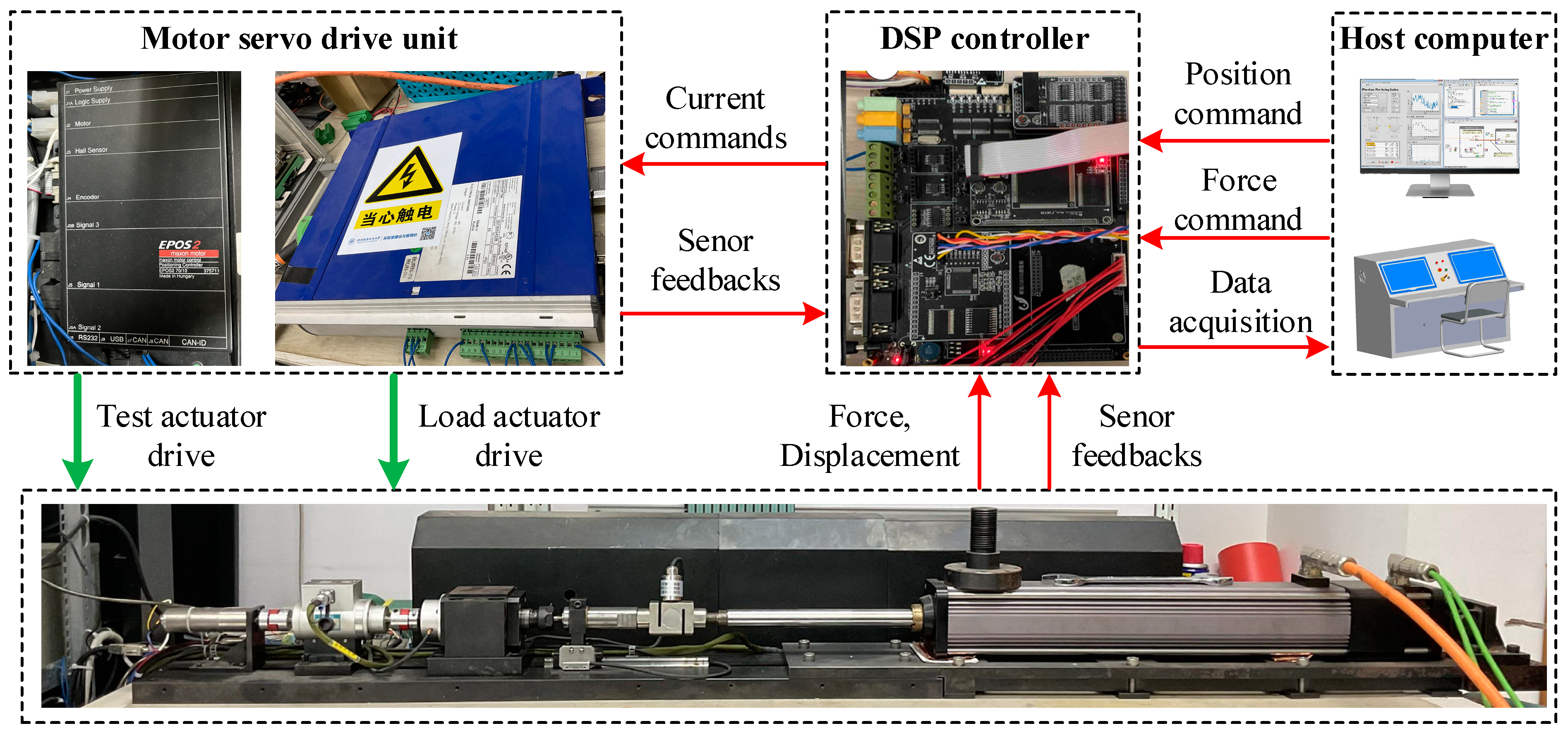
5.1. Experimental Setup

The experimental validation platform for ELLS is shown as Figure 4. The ELLS serves for the dynamic performance evaluation of EMA, responsible for the open/close operation of ram air inlet deflector door on a military aircraft. The equivalent stroke and maximum speed of the EMA operation is 30 mm and 4 mm/s, respectively. The left part is the actuator under test, which is mainly composed of DC motor, planetary reducer and screw-nut mechanism. The right part is the ELLS.

The motor angle/velocity of ELLS, linear position/speed of tested actuator and the loading force are, respectively, available from the motor encoder, the linear displacement sensor and force sensor. The acquisition of all sensor signals and the implementation of proposed control strategy are finished by DSP based controller. The control outputs are transmitted to motor servo drives as current command value. The maximum operation current for ELLS is 10 A, and the supply voltage of its servo drive unit is 270 V. A host computer is in charge of the command generation, operation state monitoring, data display and storage.

5.2. Experimental Results Analysis

Three comparative experiments are conducted to demonstrate the effectiveness of the proposed control scheme. The tested actuator is command to stay stationary or track a sinusoidal speed command, which, respectively, corresponds static and dynamic loading modes. The ELLS is controlled with the proposed OBAC and widely used PID plus velocity feedforward (PID + VF) methods. To evaluate the importance of adopting the adaptive control law to suppress the parameter uncertainties, the fixed friction compensation (FFC) method is also used for comparison.

The friction parameters constantly hold the identified value in FFC approach. The sinusoidal wave signal is introduced as the load force command with amplitude 500 N, center value −600 N and frequency 0.5 Hz. To synthetically and quantitively compare the differences of different control approaches, the following performance indexes are referred, including amplitude attenuation (AA), phase lag (PL), maximum tracking error (MTE) and mean standard error (MSE):

$$\{\begin{array}{l}\mathrm{AA}=\frac{M_{\mathrm{C}}-M_{\mathrm{L}}}{M_{\mathrm{C}}}\times 100\%\\ \mathrm{MTE}=\max (e_1)\\ \mathrm{MSE}=\frac{1}{N}\sqrt{{\displaystyle \sum _{i=1}^N{(F_{\mathrm{Lc}}-F_{\mathrm{L}})}^2}}\end{array}$$

(59)

where M_C and M_L are amplitudes of force command and response, respectively. N is the total data numbers.

The system inherent parameters participating the controller design are given as follows: J = 2.6 × 10⁻³ kg·m², k_t = 1.65 N·m/A, l_s = 2.54 × 10⁻³ m. The control and adaptive gain coefficients are set as k₁ = 0.003, k₂ = 750, λ₀ = k₃ = 0.001. The filter constant τ of the dynamic surface, the cut off frequency ω_c and bandwidth of ESO ω₀ are selected as 0.01, 35 and 120, respectively.

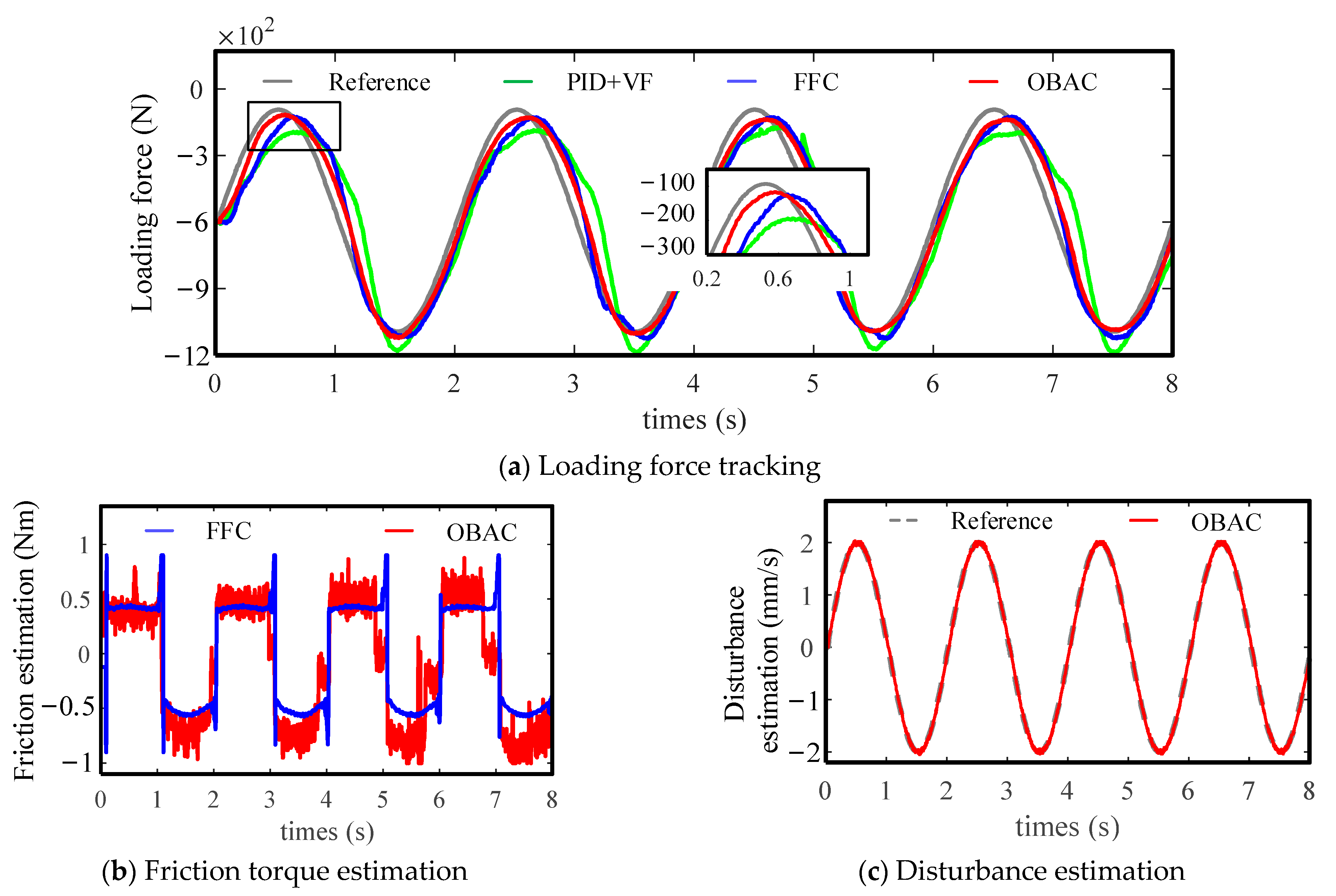
5.2.1. Static Loading Experiment

The response results of static loading experiment are depicted in Figure 5. From Figure 5a, an obvious dead zone occurs at the peak and trough of the force tracking curve under PID + VF approach. Both FFC and OBAC approaches show improvements on different levels.

However, only with the proposed OBAC approach, the dead zone phenomenon can be almost eliminated by adopting the adaptive friction compensation. The loading error and the phase lag are apparently improved at the same time. The above-mentioned criteria AA, PL, E_m and S_e are used to further evaluate the tracking performance in

Table 2. Performance indexes at static loading experiment.

	AA	PL (°)	MTE (N)	MSE (N)
NFC	7.8%	41.0	345.5	157.4
FFC	2.2%	29.8	277	118.8
OBAC	−2.2%	17.8	155	74.5

. This comprehensive comparison proves that the OBAC method possesses the best control performance at static loading.

The friction toque observation results by FFC and OBAC methods in Figure 5b are roughly consistent. The latter shows a small scale oscillation, which can be explained that the OBAC considers the friction parameter uncertainties and adopts the parameter adaptive law to improve robustness. This is why the OBAC presents better friction compensation performance than FFC. The lumped position disturbance obtained by ESO in Figure 5c is mainly composed of the unknown disturbance with relatively small value in ‘loading’ subsystem, since the tested actuator is command to stay stationary. It is noted that this disturbance is transformed to impose a speed unit for analysis convenience.

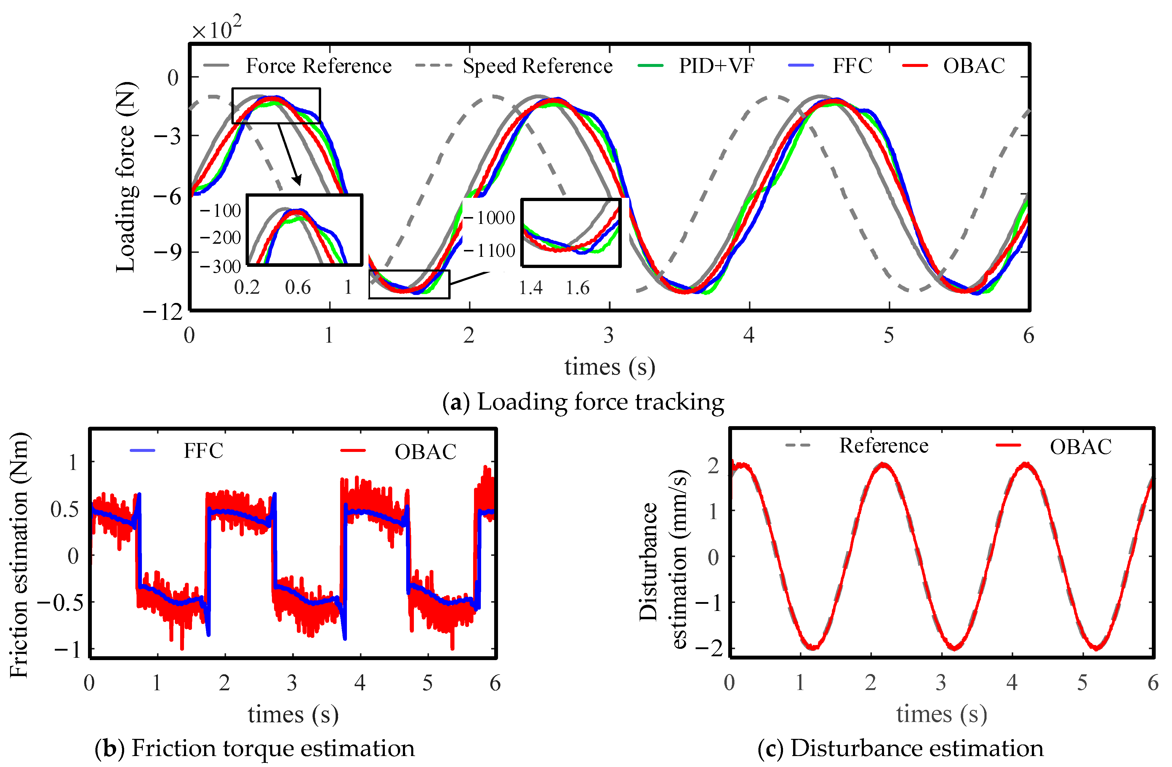
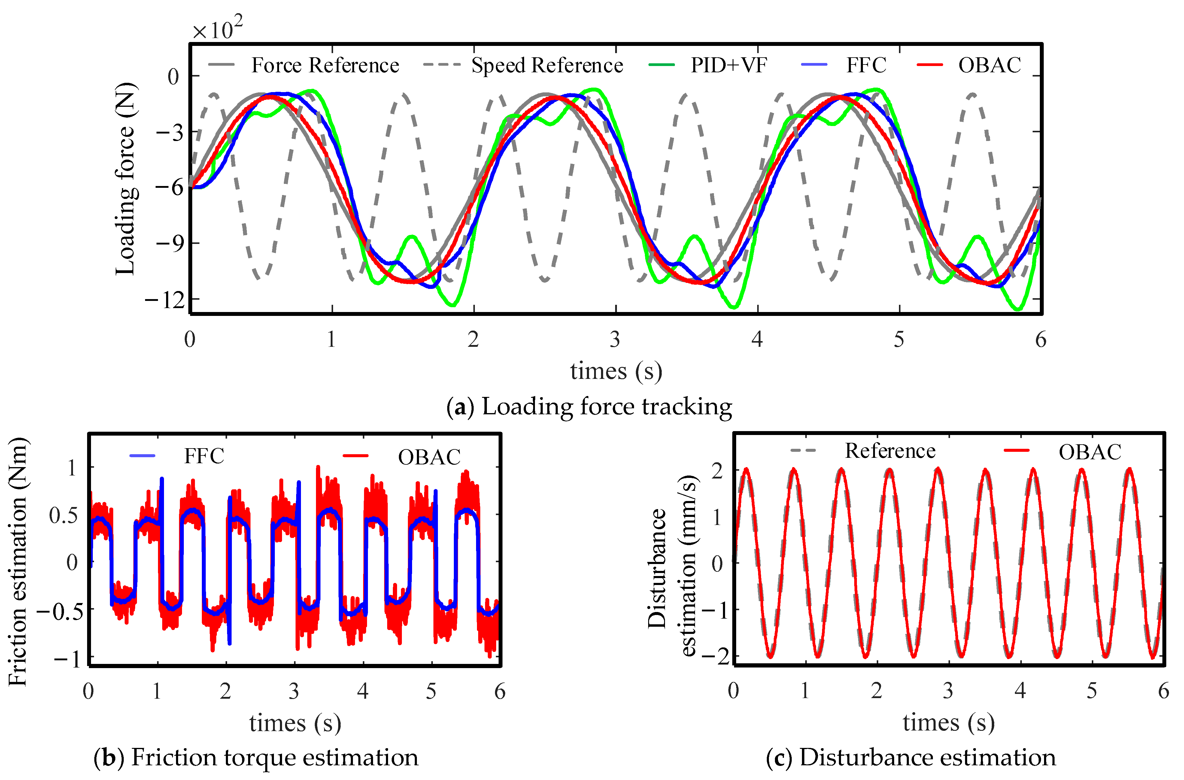
5.2.2. Dynamic Loading Experiment

At the dynamic loading experiment, the actuator under test operates under a sinusoidal speed command with amplitude 2 mm/s and frequency 0.5 Hz. The response results are depicted in Figure 6. Due to the active motion of the tested actuator, the flat-top phenomenon is weakened comparing to static loading experiment. As shown in Figure 6a, the proposed OBAC approach still presents apparent superiority at the loading error and the phase lag indexes than PID + VF and FFC methods. The respective experimental results of each index are also obtained and collected in

Table 3. Performance indexes at dynamic loading experiment.

	AA	PL (°)	MTE (N)	MSE (N)
NFC	14.4%	41.6	337.5	143.5
FFC	4.8%	27.6	228.5	93.2
OBAC	3.2%	18.7	138.2	53.6

. It is clear that the dynamic performance is significantly improved via using OBAC method. This comprehensive comparison further demonstrates the effective of the OBAC method.

Comparing to FFC, the OBAC approach considers the friction parameter uncertainties and adopts the parameter adaptive law to improve robustness, which is why the similar oscillation phenomenon of friction torque estimation exists in Figure 6b. The transition from static to coulomb friction, i.e., the Stribeck curve, is observed, when the motion speed gradually increases.

As the improved LuGre model takes the load effect into consideration, instead of an approximately constant value, the coulomb friction torque amplitude shares similar variation trends with the load force. The lumped position disturbance estimation result accomplished by ESO in Figure 6c shows great consistence with the tested actuator speed command, which proves the designed ESO is stable along with small enough observer error. The estimation result implies that the primary source of lumped position disturbance comes from the active motion of tested actuator, rather than the unknow disturbance.

It is noted that the phase and frequency of operation command for tested EMA is consistent with the loading force command, which is the most favorable case for the load simulator. However, to completely validate the effective of the proposed OBAC control strategy, the disturbances in relation to the forced motion, which may operate in out of phase or at different frequencies, must be taken into consideration. Therefore, another two dynamic loading experiments are conducted with modified operation commands for tested actuator, where the initial phase and frequency are set to pi/3 and 1.5 Hz, respectively.

The experimental results, including loading force tracking responses, friction torque estimations and disturbance estimations, are displayed in Figure 7 and Figure 8. The performance comparisons of each index are also collected in

Table 4. Performance indexes for the dynamic loading experiment (out-of-phase operation for tested EMA).

	AA	PL (°)	MTE (N)	MSE (N)
NFC	7.1%	28.8.	293.0	120.3
FFC	0.9%	21.6	271.5	134.8
OBAC	1.8%	13.7	136.2	70.6

and

Table 5. Performance indexes for the dynamic loading experiment (different frequency operation for tested EMA).

	AA	PL (°)	MTE (N)	MSE (N)
NFC	−4.9%	61.2	442.5	196.1
FFC	−0.7%	24.3	256.0	136.5
OBAC	2.5%	12.6	117.7	63.6

. It is obvious that the dynamic performance via using OBAC method is superior. The designed ESO can still accurately obtain the lumped position disturbance caused by forced motion of tested actuator in Figure 7c and Figure 8c.

There are certain other phenomena worth noting, with the existence of phase and frequency differences between forced motion command and loading force command. Due to the phase difference, the stick-slip friction variation is coupled into the ELLS, when the loading force response experiences a peak or trough.

In partial enlarged drawing of Figure 7a, if the NFC approach is adopted, the ‘flat top’ and distortion phenomenon of force tracking curve is more apparent than that in Figure 6a. In addition, with the forced motion frequency increases to three times of loading frequency, the friction disturbance is much stronger with high-frequency and complex variations of direction and magnitude. Therefore, the tracking performance is seriously influenced in Figure 8a, if no friction compensation strategy (NFC method) is used.

Finally, compared to the OBAC approach, it can be observed that the loading force tracking via FFC controller exist larger phase lags and distortion phenomena in Figure 7a and Figure 8a, which can be explained by friction torque estimation differences in Figure 7b and Figure 8b. The fundamental reason is that the OBAC method utilizes the parameter adaptive law to suppress friction parameter uncertainties, which leads to better friction compensation performance.

6. Conclusions

(1)

Under the influence of friction nonlinearity, position disturbance and parameter uncertainties, an observer-based backstepping adaptive control (OBAC) strategy was proposed to achieve high-load force tracking performance for an electro-mechanical actuator. The whole system was divided into ‘actuation’ and ‘loading’ subsystems with the backstepping design concept. The dynamic control surface was introduced to solve the so-called differential explosion problem.

(2)

The estimation of the position disturbance was obtained by an extended stated observer and used for feedforward compensation for the ‘loading’ subsystem. For the ‘actuation’ subsystem, a friction scale factor with a reasonable adaptive updating law was introduced to reject the disturbance of the friction parameter uncertainties for both simplified and effective purposes. Combining the observer for internal state of friction model and an improved LuGre based friction model, which considers the load influence on friction, adaptive friction compensation was conducted.

(3)

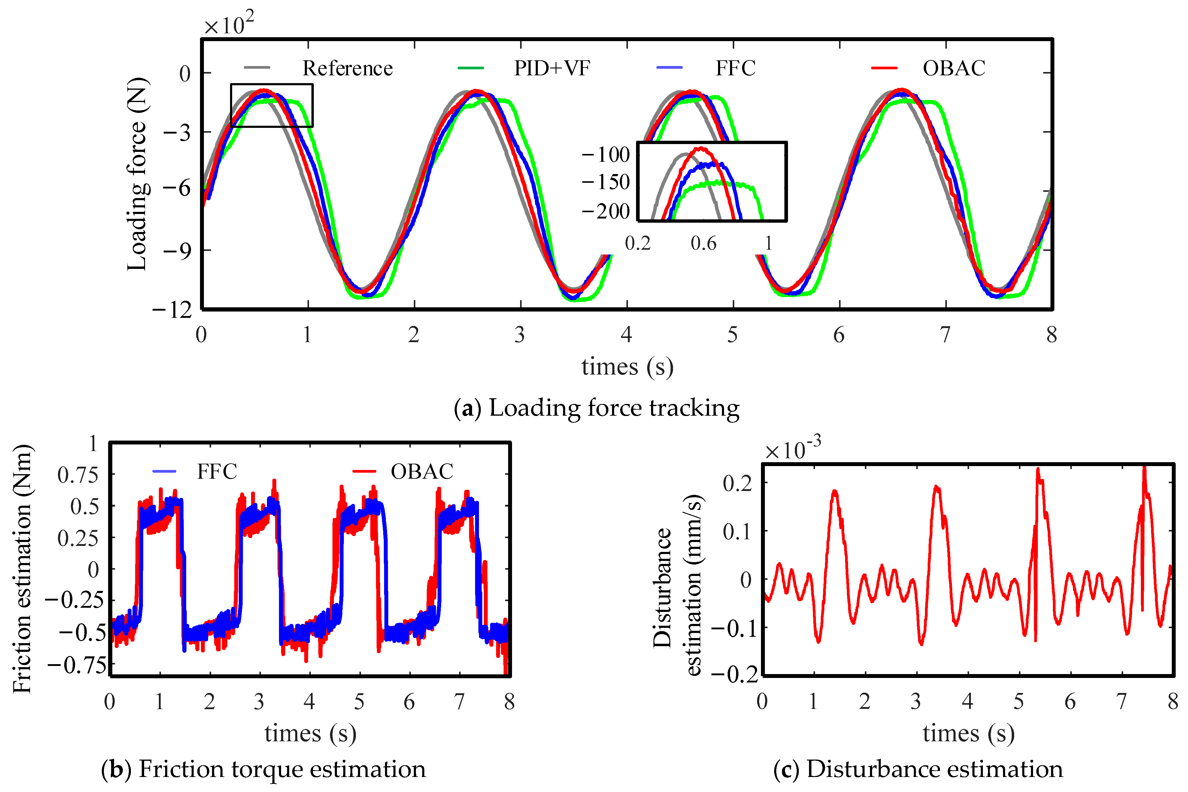
The static and three different types of dynamic loading experiments sufficiently verified that the proposed OBAC control strategy achieved high-precision load force tracking and strong robustness. The designed ESO accurately obtained the lumped position disturbance caused by forced motion of the tested actuator. By using the friction torque estimation for compensation, the ‘flat-top’ or distortion phenomenon can be eliminated or weakened. Compared to the FFC approach, the proposed OBAC method utilizes the parameter adaptive law to suppress friction parameter uncertainties, which leads to superior performance of the loading force control.

References

1. Mare, J.C.; Fu, J. Review on signal-by-wire and power-by-wire actuation for more electric aircraft. Chin. J. Aeronaut. 2017, 30, 857–870. [Google Scholar] [CrossRef]
2. Qiao, G.; Liu, G.; Shi, Z.; Wang, Y.; Ma, S.; Lim, T.C. A Review of Electromechanical Actuators for More/All Electric Aircraft Systems. Proc. Inst. Mech. Eng. Part C J. Eng. Mech. Eng. Sci. 2017, 232, 4128–4151. [Google Scholar] [CrossRef] [Green Version]
3. Bajcinca, N.; Schurmann, N.; Bals, J. Two degree of freedom motion control of an energy optimized aircraft ram air inlet actuator. In Proceedings of the International Conference on Control and Automation (ICCA), Budapest, Hungary, 26–29 June 2005; pp. 818–821. [Google Scholar]
4. SAE Aerospace. Trimmable Horizontal Stabilizer Actuator Descriptions: SAE AIR6052; SAE International: Warrendale, PA, USA, 2011; pp. 1–38. [Google Scholar]
5. Jensen, S.C.; Jenney, G.D.; Dawson, D. Flight Test Experience with an Electromechanical Actuator on the F-18 Systems Research Aircraft. In Proceedings of the 19th Digital Avionics Systems Conference (DASC), Philadelphia, PA, USA, 7–13 October 2000; pp. 1–10. [Google Scholar]
6. Todeschi, M. Airbus-EMAs for Flight Controls Actuation System-An Important Step Achieved in 2011; SAE Technical Paper 2011-01-2732; SAE International: Warrendale, PA, USA, 2011; Volume 1. [Google Scholar]
7. Jiménez, A.; Lasa, J.; Novillo, E.; Eguizabal, I.; Aguado, F.; Lopez, I. Electromechanical Actuator with Anti-Jamming System for Safety critical aircraft applications. In Proceedings of the 7th International Conference on Recent Advances in Aerospace Actuation Systems and Components, Toulouse, France, 16–18 March 2016; pp. 27–32. [Google Scholar]
8. Whitley, C.; Ropert, J. Development, manufacture & flight test of spoiler EMA system. In Proceedings of the 3rd International Conference on Recent Advances in Aerospace Actuation Systems and Components, Toulouse, France, 13–15 June 2007; pp. 215–220. [Google Scholar]
9. Bohr, G.; Hamilton, S. Force control is the issue in aerospace structural test lab. Hydraul. Pneum. 2000, 53, 43–47. [Google Scholar]
10. Nam, Y.; Sung, K. Force control system design for aerodynamic load simulator. Control Eng. Pract. 2002, 10, 549–558. [Google Scholar] [CrossRef]
11. Arena, M.; Amoroso, F.; Pecora, R.; Ameduri, S. Electro-Actuation System Strategy for a Morphing Flap. Aerospace 2019, 6, 1. [Google Scholar] [CrossRef] [Green Version]
12. Mare, J.C. Dynamic loading systems for ground testing of high speed aerospace actuators. Aircr. Eng. Aerosp. Tec. 2006, 78, 275–282. [Google Scholar] [CrossRef]
13. Kang, S.; Yan, H.; Dong, L.; Li, C. Finite-time adaptive sliding mode force control for electro-hydraulic load simulator based on improved GMS friction model. Mech. Syst. Signal Process. 2018, 102, 117–138. [Google Scholar] [CrossRef]
14. Matsui, T.; Mochizuki, Y. Effect of positive angular velocity feedback on torque control of hydraulic actuator. Trans. Jpn. Soc. Mech. Eng. 2008, 57, 1604–1609. [Google Scholar]
15. Zheng, S.; Fu, Y.; Wang, D.; Zhang, W.; Pan, J. Investigations on system integration method and dynamic performance of electromechanical actuator. Sci. Prog. 2020, 103, 03685042094092. [Google Scholar] [CrossRef] [PubMed]
16. Yao, J.; Jiao, Z.; Han, S. Friction compensation for low velocity control of hydraulic flight motion simulator: A simple adaptive robust approach. Chin. J. Aeronaut. 2013, 26, 814–822. [Google Scholar] [CrossRef] [Green Version]
17. Yao, J.; Jiao, Z.; Yao, B. Robust Control for Static Loading of Electro-hydraulic Load Simulator with Friction Compensation. Chin. J. Aeronaut. 2012, 25, 954–962. [Google Scholar] [CrossRef] [Green Version]
18. Alleyne, A.; Liu, R. A simplified approach to force control for electro-hydraulic systems. Control Eng. Pract. 2000, 8, 1347–1356. [Google Scholar] [CrossRef]
19. Wang, C.; Jiao, Z.; Quan, L.; Meng, H. Application of adaptive robust control for electro-hydraulic motion loading system. Trans. Inst. Meas. Control 2018, 40, 873–884. [Google Scholar]
20. Wang, L.; Wang, M.; Guo, B.; Wang, Z.; Wang, D.; Li, Y. A Loading Control Strategy for Electric Load Simulators Based on Proportional Resonant Control. IEEE Trans. Ind. Electron. 2018, 65, 4608–4618. [Google Scholar] [CrossRef]
21. Zhao, J.; Shen, G.; Zhu, W.; Yang, C.; Yao, J. Robust force control with a feed-forward inverse model controller for electro-hydraulic control loading systems of flight simulators. Mechatronics 2016, 38, 42–53. [Google Scholar] [CrossRef]
22. Jing, C.; Xu, H.; Jiang, J. Dynamic surface disturbance rejection control for electro-hydraulic load simulator. Mech. Syst. Signal Process. 2019, 134, 1026293. [Google Scholar] [CrossRef]
23. Niksefat, N.; Sepehri, N. Design and experimental evaluation of a robust force controller for an electro-hydraulic actuator via quantitative feedback theory. Control Eng. Pract. 2000, 8, 1335–1345. [Google Scholar] [CrossRef]
24. Truong, D.Q.; Ahn, K.K. Force control for hydraulic load simulator using self-tuning grey predictor fuzzy PID. Mechatronics 2009, 19, 233–246. [Google Scholar] [CrossRef]
25. Li, C.; Pan, X.; Wang, G. Torque tracking control of electric load simulator with active motion disturbance and nonlinearity based on T-S fuzzy model. Asian J. Control 2018, 22, 1280–1294. [Google Scholar] [CrossRef]
26. Li, C.; Li, Y.; Wang, G. H-infinity output tracking control of Electric-motor-driven aerodynamic Load Simulator with external active motion disturbance and nonlinearity. Aerosp. Sci. Technol. 2018, 82–83, 334–349. [Google Scholar] [CrossRef]
27. de Wit, C.C.; Olsson, H.; Astrom, K.; Lischinsky, P. A new model for control of systems with friction. IEEE Trans. Autom. Control 1995, 40, 419–425. [Google Scholar] [CrossRef] [Green Version]
28. Fu, J.; Maré, J.C.; Fu, Y. Modelling and Simulation of Flight Control Electromechanical Actuators with Special Focus on Model Architecting, Multidisciplinary Effects and Power Flows. Chin. J. Aeronaut. 2017, 30, 47–65. [Google Scholar] [CrossRef] [Green Version]
29. Ping, Z.; Zhang, W.; Fu, Y. Improved LuGre-based friction modeling of the electric linear load simulator. In Proceedings of the 8th International Conference on Manufacturing Technology and Applied Materials (ICAMMT), Hangzhou, China, 15–17 April 2022. [Google Scholar]
30. Wang, X.; Wang, S. High Performance Adaptive Control of Mechanical Servo System with LuGre Friction Model: Identification and Compensation. J. Dyn. Syst. Meas. Control 2012, 134, 011021. [Google Scholar] [CrossRef] [Green Version]
31. Chen, Q.; Chen, H.; Zhu, D.; Li, L. Design and Analysis of an Active Disturbance Rejection Robust Adaptive Control System for Electromechanical Actuator. Actuators 2021, 10, 307. [Google Scholar] [CrossRef]
32. Xu, D.; Huang, J.; Su, X.; Shi, P. Adaptive command-filtered fuzzy backstepping control for linear induction motor with unknown end effect. Inf. Sci. 2019, 477, 118–131. [Google Scholar] [CrossRef]
33. Swaroop, D.; Hedrick, J.K.; Yip, P.P.; Gerdes, J. Dynamic surface control for a class of nonlinear systems. IEEE Trans. Autom. Control 2002, 45, 1893–1899. [Google Scholar] [CrossRef] [Green Version]
Figure 1. Architecture of the ELLS and tested actuator.
Aerospace 09 00415 g001
Figure 2. Identification results of friction parameters. (a) Experimental and identification results of friction with static parameters. (b) Experimental and identification results of pre-slip displacement with dynamic parameters.
Aerospace 09 00415 g002
Figure 3. The architecture of the proposed observer-based adaptive backstepping controller.
Aerospace 09 00415 g003
Figure 4. Experimental validation platform for ELLS.
Aerospace 09 00415 g004
Figure 5. Static loading experiment results with different control methods.
Aerospace 09 00415 g005
Figure 6. Dynamic loading experiment results with different control methods.
Aerospace 09 00415 g006
Figure 7. Dynamic loading experiment results (out-of-phase operation for tested EMA).
Aerospace 09 00415 g007
Figure 8. Dynamic loading experiment results (different frequency operation for tested EMA).
Aerospace 09 00415 g008