Aircraft Lateral-Directional Aerodynamic Parameter Identification and Solution Method Using Segmented Adaptation of Identification Model and Flight Test Data

Abstract

Current aerodynamic parameter identification methods take the consistency between the response of the motion model reconstructed with the identified aerodynamic parameters and flight data as an optimization index. Since there is only one index constraint in aerodynamic parameter optimization, and more than ten aerodynamic parameters to be identified simultaneously have different sensitivity to the optimization index, the accuracy of identification results of parameters with low sensitivity is poor, especially for those with small absolute value. To solve these problems, a new idea, having aerodynamic parameters solved by balance equations and identified in stages, is proposed. Based on the motion characteristics of different lateral-directional maneuvers, the scheme of combined maneuvers is designed, and the step-by-step identification procedure is established. An estimation method of angular acceleration with angular velocity equivalent model is proposed to solve the problem that angular acceleration cannot be measured directly. A lateral-directional aerodynamic parameter identification method using segmented adaptation of flight data and identification models is established based on the identifiability of flight data. The lateral-directional aerodynamic parameter identification results of a large civil aircraft show the identification results can be obtained with higher accuracy by adopting the proposed identification method and the flight test scheme.

1. Introduction

The aim of aircraft aerodynamic parameter identification is to obtain an accurate aerodynamic model through valid content in flight data [1,2]. The widely used parameter identification methods, such as the maximum likelihood estimation (MLE) method, carry out the optimization of multiple objectives under only one constraint. All of them take the likelihood function established based on the identification model’s response and flight data as an optimization index. They are carried out by simultaneously iterating all unknown aerodynamic derivatives (generally more than ten) in the identification model. Since all of the parameters to be identified have different sensitivity to the change of the only constraint index, the optimal solution, during different time periods, obtained from the flight test data of the same aircraft in the same flight state, is not the same. As a result, the consistency of identification results is poor, especially for some aerodynamic derivatives such as C_nδa and C_lr with low sensitivity to the change of the optimization constraint index and small absolute value. Furthermore, the accuracy of identification results is low [3,4,5]. In the flight dynamics modeling of a civil aircraft flight simulator, some objective tests of qualification performance standards in airworthiness regulations, such as step input of flight deck roll controller, spiral stability [6], etc., require derivatives such as C_nδa and C_lr of a higher accuracy. Using existing conventional aerodynamic parameter identification methods, it is often difficult to meet the accuracy requirements of objective tests of qualification performance standards.

In order to solve this problem, reference [7] presents an identification and solution method of aerodynamic derivatives, where the derivatives are identified/solved step-by-step using data from different flight test maneuvers. It has been applied in the aerodynamic modeling of simulators in recent years. The basic principle of the method is to identify different derivatives in stages by using the various dynamic characteristics of aircraft in different flight test maneuvers, and the accurate results obtained are used as prior information for the identification and solution of subsequent derivatives. More specifically, the control derivatives and stability derivatives are identified and solved through asymmetric thrust trim, steady heading sideslip (SHSS), roll response, rudder response and Dutch roll, respectively. Then, using the obtained derivative identification results as prior information, the dynamic derivatives are identified by exciting Dutch-roll oscillation. Due to the fact that only a few derivatives are identified through each flight test maneuver, and the relatively accurate results obtained can be used as the prior constraints for the subsequent derivative identification, the disadvantage of the conventional methods is circumvented by transforming the multi-objective optimization into the identification and solution of a small number of derivatives under multiple constraints. This improves the accuracy of the identification results effectively.

However, this step-by-step identification/solution approach also has some shortcomings. First, the flight test scheme is complicated, requiring at least five kinds of flight test maneuvers, as mentioned above. Secondly, asymmetric thrust trim is the basis of the identification and solution process. This maneuver requires the engines on both sides to provide sufficient and accurately measured asymmetric thrust for the calculation of C_nβ and C_nδr. However, for aircraft with a single engine or short engine distance (i.e., the distance between the engines on both sides of the aircraft and the symmetrical plane of the aircraft is short), the lateral-directional aerodynamic derivatives cannot be the identified accurately by this method. Thus, the application scope of this method is limited. In addition, reference [7] only provides the specific steps for solving stability derivatives and control derivatives based on the balance equations without providing specific procedures for identification of dynamic derivatives.

A new step-by-step identification method is proposed without using asymmetric thrust trim. The lateral-directional aerodynamic derivatives of the aircraft can be accurately obtained through SHSS and 3-2-1-1 input of aileron and rudder. Firstly, the identification procedure is designed to obtain all the derivatives according to the valid content of aerodynamic parameters in the flight test data of the above three maneuvers. Then, according to the change of the magnitude of each variable, all flight data are divided into different data segments. This is because only the data with large magnitude of variables and no collinearity could have better identifiability. In some cases, it is necessary to select discontinuous data segments for identification in order to obtain data with larger magnitude and better identifiability, since the aerodynamic forces and moments of the aircraft constantly change. The maximum likelihood estimation (MLE) method cannot be used for identification of discontinuous data [8]; hence, the least squares method is used for parameter identification, which makes it necessary to use accurate angular acceleration data to calculate aerodynamic moment coefficients. However, it is difficult to measure angular acceleration directly and accurately because of the immaturity of current angular acceleration measurement technology [9,10]. Meanwhile, differential angular velocity data will produce differential error and greatly magnify data noise [11], so the obtained differential data cannot be used for identification. To obtain angular acceleration data with high accuracy, an angular acceleration estimation method based on the angular velocity equivalent model (AVEM) is proposed. Firstly, based on the generic aerodynamic moment model and the rotational dynamics equations of aircraft, an AVEM is established, which could fit the flight test data of aircraft angular velocity well. Then, the time delay between angular velocity data and control surface deflection data is calibrated using the cross-correlation function between the angular acceleration response (AAR) of the AVEM and the differential signal of angular velocity data. Finally, the angular acceleration calculated through the AVEM is used as the estimated value of the aircraft’s angular acceleration during flight tests.

Flight data will be segmented preliminarily according to the change of the magnitude of each variable, and the stepwise regression and the combined model-fitting evaluation metrics are used to determine the model structure and the data segmentation scope. The unidentifiable terms will be processed as colored noise. According to the designed identification and solution procedure, the identification and solution of lateral-directional aerodynamic derivatives are carried out in stages using the ordinary least squares method and least squares mixed estimator. Meanwhile, C_lβ and C_nδa are directly solved through prior constraints and SHSS trim results. Finally, the established identification/solution method, which adopts the segmented adaptation of flight test data and identification models, is used to identify and validate the lateral-directional aerodynamic parameters based on the flight test data of a large fly-by-wire-controlled civil aircraft. The results are compared and analyzed with lateral-directional aerodynamic parameters obtained from the conventional MLE method.

2. Identification Principle of Aerodynamic Parameters Based on Combined Maneuvers Scheme

2.1. Principle of Aerodynamic Parameter Identification

The identification model of lateral-directional aerodynamic parameters includes side force, roll and yaw moment:

$$\{\begin{array}{l}{C}_Y=C_{Y\beta }\beta +C_{Y{\delta }_r}{\delta }_r+C_{Yr}\overline{r}+C_{Yp}\overline{p}\\ C_l=C_{l\beta }\beta +C_{l{\delta }_r}{\delta }_r+C_{l{\delta }_a}{\delta }_a+C_{lp}\overline{p}+C_{lr}\overline{r}\\ C_n=C_{n\beta }\beta +C_{n{\delta }_r}{\delta }_r+C_{n{\delta }_a}{\delta }_a+C_{np}\overline{p}+C_{nr}\overline{r}\end{array}$$

(1)

The independent variables of the lateral-directional aerodynamic parameter identification model are the motion variables and control surface deflections in Equation (1). The observation variables of the identification model are side force coefficient C_Y, roll moment coefficient C_l and yaw moment coefficient C_n.

$$\{\begin{array}{l}{C}_Y=\frac{Y}{0.5\rho V^{2}S}=\frac{m{a}_y}{0.5\rho V^{2}S}\\ C_l=\frac{L}{0.5\rho V^{2}Sb}=\frac{\dot{p}{I}_{xx}+qr(I_{zz}-I_{yy})-(pq+\dot{r})I_{xz}}{0.5\rho V^{2}Sb}\\ C_n=\frac{N}{0.5\rho V^{2}Sb}=\frac{\dot{r}{I}_{zz}+pq(I_{yy}-I_{xx})+(qr-\dot{p})I_{xz}}{0.5\rho V^{2}Sb}\end{array}$$

(2)

The mass, inertial moment, dynamic pressure, lateral acceleration and angular velocity in Equation (2) could be measured in the aerodynamic parameter identification flight test. Angular acceleration is estimated through the method described in Section 2.2. To sum up, the data of C_Y, C_l and C_n are calculated from the directly measured flight test data and the estimated angular acceleration in the identification model. Because these data are essentially objective observations of the aerodynamic forces and moments of the aircraft in the motion, they are called observations.

In order to simplify the flight test scheme, it is necessary to accurately identify multiple derivatives through a single maneuver. The 3-2-1-1 signal is easily executed for the control surfaces of the aircraft, and its response has sufficient content of dynamic characteristics. The response data of different segments show different dynamic characteristics of the aircraft, which can be used to identify different derivatives. On the basis of this, the three flight test maneuvers adopted for identification of the lateral-directional aerodynamic derivatives of aircraft in this paper are aileron, rudder 3-2-1-1 signal input and SHSS. The typical 3-2-1-1 signal includes four continuous square-wave signals with durations of 3 s, 2 s, 1 s and 1 s and amplitudes of positive, negative, positive and negative, respectively, as shown in Figure 1:

The 3-2-1-1 aileron input can fully excite the roll motion of the aircraft, which is beneficial to the identification of the aileron roll control derivative and the dynamic derivative related to the roll angle velocity [12]. At the initial response stage, the roll motion is mainly generated by the aileron roll control moment and roll damping moment, since the sideslip angle and yaw angular velocity generated by aileron deflection are small. In such a case, the roll moment coefficient of the aircraft can be expressed as:

$$\{\begin{array}{l}{C}_l=C_{l{\delta }_a}{\delta }_a+C_{lp}\overline{p}+\Delta C_l\\ \Delta C_l=C_{l\beta }\beta +C_{l{\delta }_r}{\delta }_r+C_{lr}\overline{r}\end{array}$$

(3)

In Equation (3), ΔC_l represents the components of the rolling moment with relatively little effect on the rolling motion. The sensitivity of C_l to C_lδa can be improved effectively by using the initial response data of the 3-2-1-1 aileron input.

At the initial response stage of 3-2-1-1 rudder input, the yaw and roll angular velocity caused by control are small, and the motion is mainly generated by the rudder control moment and directional stability moment. In such a case, the roll and yaw moment coefficient can be expressed as:

$$\{\begin{array}{l}{C}_l=C_{l{\delta }_r}{\delta }_r+C_{l\beta }\beta +\Delta C_l\\ \Delta C_l=C_{lr}\overline{r}+C_{lp}\overline{p}\end{array}$$

(4)

$$\{\begin{array}{l}{C}_n=C_{n{\delta }_r}{\delta }_r+C_{n\beta }\beta +\Delta C_n\\ \Delta C_n=C_{nr}\overline{r}+C_{np}\overline{p}\end{array}$$

(5)

In Equation (5), ΔC_n represents the components of the yaw moment with relatively little effect on the yaw motion. The sensitivity of C_n and C_l to C_lδr and C_nδr can be improved effectively by using the initial response data of the 3-2-1-1 rudder input.

After the initial response stage of the 3-2-1-1 rudder input, the control of the rudder will cause significant lateral-directional coupling motion, and sideslip angle, roll and yaw angular velocity will change significantly. In such a case, the side force, roll and yaw moment coefficient can be expressed as:

$$\{\begin{array}{l}{C}_Y=C_{Y\beta }\beta +C_{Y{\delta }_r}{\delta }_r+C_{Yr}\overline{r}+C_{Yp}\overline{p}\\ C_l=C_{l{\delta }_r}{\delta }_r+C_{l\beta }\beta +C_{lr}\overline{r}+C_{lp}\overline{p}\\ C_n=C_{n{\delta }_r}{\delta }_r+C_{n\beta }\beta +C_{nr}\overline{r}+C_{np}\overline{p}\end{array}$$

(6)

C_nr, C_Yβ and C_Yδr are identified by Equation (6). The impact of β and δ_r measurement error in identification of C_nr can be reduced by using the identification results of C_nδr and C_nβ already obtained. In the response to rudder input, the accuracy of identification results of cross derivatives is relatively low. This is based on the fact that the lateral-directional motion coupling is obvious, and the aerodynamic moment components affecting the aircraft motion are so complex that the cross moment is not the dominant moment for the roll and yaw motion. After the identification of control derivatives, stability derivatives and damping derivatives, the identification accuracy of cross derivatives can be effectively improved by taking the identification results as prior information and selecting the data with large angular velocity, relatively small sideslip angle, and small control surface deflection.

The sideslip angle in SHSS is stable and has relatively small observation error. However, the change of sideslip angle and rudder surface deflection angle presents a stable linear feature. It means that the data has collinearity and cannot be used for identification under general conditions. However, this ratio relation can be used as a prior constraint for the solution of C_lβ and C_nβ after the control derivatives are obtained by the identification of other maneuvers. The lateral-directional aerodynamic force and moment balance equations in SHSS are the following:

$$\{\begin{array}{l}{C}_Y=C_{Y\beta }\beta +C_{Y{\delta }_r}{\delta }_r=m{a}_y/(0.5\rho V^{2}S)\\ C_l=C_{l\beta }\beta +C_{l{\delta }_r}{\delta }_r+C_{l{\delta }_a}{\delta }_a=0\\ C_n=C_{n\beta }\beta +C_{n{\delta }_r}{\delta }_r+C_{n{\delta }_a}{\delta }_a=0\end{array}$$

(7)

The ratio relationship among aileron deflection, rudder deflection and sideslip angle in SHSS can be gained through Equation (7). C_lβ can be directly solved by using the obtained C_lδa and C_lδr, and C_nδa can be directly solved by using the obtained C_nδr and C_nβ. Furthermore, C_np is identified through the 3-2-1-1 aileron input response data, and C_lr is identified through the 3-2-1-1 rudder input response data based on the identification results obtained through the steps above.

To sum up, the scheme of combined flight test maneuvers for identification of lateral-directional aerodynamic parameters is as follows: Firstly, C_lδa and C_lp are identified through the 3-2-1-1 aileron input. Next, C_lδr, C_nδr, C_nβ, C_nr, C_Yβ and C_Yδr are identified through the 3-2-1-1 rudder input. Thirdly, C_lβ is solved by using SHSS flight data and the identification results of C_lδa and C_lδr. C_nδa is solved by using SHSS flight data and the identification results of C_nδr and C_nβ. Finally, C_np is identified by using the flight data of the 3-2-1-1 aileron input and the identification results of C_nδa, C_nδr, C_nβ and C_nr. C_lr is identified by using the flight data of the 3-2-1-1 rudder input and the identification results of C_lδr, C_lβ and C_lp.

2.2. Angular Acceleration Estimation Method

In the aerodynamic parameter identification principle mentioned above, it is necessary to obtain accurate angular acceleration data to calculate the observation values of roll and yaw moment coefficients for data segmentation and parameter identification. Since angular acceleration is difficult to be measured directly and accurately, an AVEM, which can well fit the flight data of angular velocity, is established, and the calculated value of angular acceleration based on the AVEM is used as the estimated value of angular acceleration. The generic aerodynamic model, as the modeling basis of AVEM, is a polynomial model [13,14], and it includes a constant term, aerodynamic angle, angular velocity, rudder deflection angle, high-order aerodynamic angle and coupling term, etc. The structure of the generic three-axis aerodynamic moment coefficient model is [15]:

$$\{\begin{array}{l}{C}_l={\theta }_1\beta +{\theta }_2\overline{p}+{\theta }_3\overline{r}+{\theta }_4{\delta }_a+{\theta }_5{\delta }_r\\ C_m={\theta }_6+{\theta }_7\alpha +{\theta }_8\overline{q}+{\theta }_9{\delta }_e+{\theta }_{10}\alpha \overline{q}+{\theta }_{11}{\alpha }^2\overline{q}+{\theta }_{12}{\alpha }^2{\delta }_e+{\theta }_{13}{\alpha }^3\overline{q}+{\theta }_{14}{\alpha }^3{\delta }_e+{\theta }_{15}{\alpha }^4\\ C_n={\theta }_{16}\beta +{\theta }_{17}\overline{p}+{\theta }_{18}\overline{r}+{\theta }_{19}{\delta }_a+{\theta }_{20}{\delta }_r+{\theta }_{21}{\beta }^2+{\theta }_{22}{\beta }^3\end{array}$$

(8)

where θ₁~θ₂₂ are the unknown parameters in the generic aerodynamic model, which are used to describe the contribution of aerodynamic angle, angular velocity, control surface deflection and possible nonlinear factors to the aerodynamic moment coefficient. The three-axis rotational dynamics equations are the following:

$$\{\begin{array}{l}\dot{p}=\frac{C_l\overline{Q}Sb}{I_{xx}}-\frac{(I_{zz}-I_{yy})}{I_{xx}}qr+\frac{I_{xz}}{I_{xx}}(pq+\dot{r})\\ \dot{q}=\frac{C_m\overline{Q}S\overline{c}}{I_{yy}}-\frac{(I_{xx}-I_{zz})}{I_{yy}}pr-\frac{I_{xz}}{I_{yy}}(p^2-r^2)\\ \dot{r}=\frac{C_n\overline{Q}Sb}{I_{zz}}-\frac{(I_{yy}-I_{xx})}{I_{zz}}pq+\frac{I_{xz}}{I_{zz}}(\dot{p}-qr)\end{array}$$

(9)

The AVEM is constructed preliminarily by combing generic aerodynamic model (8) with the aircraft’s rotational dynamics as shown in Equation (9). The angular velocity response of the AVEM can be obtained by integrating the angular acceleration output of Equation (9). The unknown parameters in model (8) will be iterated to make the angular velocity response of the AVEM fit the angular velocity flight data. The initial values of unknown parameters corresponding to aerodynamic angle, angular velocity and control surface deflection can respectively adopt the stability derivatives, dynamic derivatives and control derivatives obtained in the wind tunnel test. Meanwhile, the initial values of the remaining unknown parameters can be set to zero. For example, the initial values of θ₁₆~θ₂₀ corresponding to β, $\overline{p}$, $\overline{r}$, δ_a and δ_r can directly adopt the wind tunnel data of C_nβ, C_np, C_nr, C_nδa and C_nδr, and the initial values of θ₂₁ and θ₂₂ corresponding to β² and β³ are 0.

The cost function transformed by the likelihood function between angular velocity response of the AVEM and angular velocity data is used as optimization index

$$J(\Theta )=\det (\mathit{R})$$

(10)

The maximum likelihood estimation of R is:

$$\mathit{R}=\frac{1}{N}{\displaystyle \sum _{k=1}^N[z(t_k)-y(t_k)]{[z(t_k)-y(t_k)]}^T}$$

(11)

where N is the data length. z(t_k) is the measurement of angular velocity data at t_k time point. y(t_k) is the output value of the AVEM at t_k time point. Iteration of the unknown parameters in model (8) is carried out by Newton–Raphson method to minimize $J(\Theta )$.

2.3. Synchronization of Control Surface Deflection Data and Angular Velocity Data

The accuracy of control surface deflection data directly affects the fitting of the AVEM to angular velocity data because the control surface deflection is one of the main inputs of model (8). Since the control surface deflection data are mainly measured by the actuator position sensor, and the angular velocity data are mainly measured by the gyroscope, they are often not synchronized; in other words, they often do not change simultaneously. This leads to poor fitting of the AVEM and low accuracy of angular acceleration estimation. Hence, it is necessary to synchronize the control surface deflection data with the angular velocity data. The measurement delay τ of angular velocity gyroscope can be approximated as [16]:

$$\tau =\frac{1}{{\omega }_f}\arctan \left(\frac{2n_s{\omega }_f}{{\omega }_f^2-{\omega }_s^2}\right)$$

(12)

where, ω_s and n_s are the natural frequency and damping of the sensor; ω_f is the frequency of aircraft motion. It is generally considered that the time delay of the measured data is negligible when ω_s is larger than 2.5ω_f [16]. The natural frequency of the gyroscope used in the flight test is 12.5 Hz, which is much higher than the frequency of aircraft motion. In this case, the delay of angular velocity data can be ignored. AAR of the AVEM and control surface deflection data change simultaneously. Angular velocity data and its differential data change simultaneously. Hence, the gap of time points at which AAR of the AVEM and differential angular velocity data change is the gap of time points at which control surface deflection data and angular velocity data change. Due to no time delay in angular velocity data and its differential data, this gap of time points is the time delay of control surface deflection data.

The differential signal of angular velocity data and AAR of the AVEM are most similar when they change simultaneously. The greater the time difference between the two signals is, the lower the similarity is. Therefore, the time delay between two signals can be determined by the normalized cross-correlation function [17]:

$$R_{xy}(m)=\frac{{\displaystyle \sum _{n=0}^{N}x(n)y(n+m)}}{{\displaystyle \sum _{n=0}^{N}x(n)x(n)}}$$

(13)

Equation (13) gives the correlation between sequence x(n), which does not move, and sequence y(n), which moves left or right on the time axis for m sampling periods. The closer R_xy is to 1, the more similar the two sequences are. Taking the sequence of differential angular velocity data as x(n) and the AVR sequence of the AVEM as y(n), the cross-correlation function between them is calculated. The m when R_xy is closest to 1 is taken as the time delay of the control surface deflection data (the time delay of the angular velocity data approximates to 0). The AVEM with better fitting can be obtained by fitting the angular velocity data again with the synchronized calibration control surface deflection data.

It should be noted that, since the AVEM is fitted by aerodynamic angle, angular velocity and other data, the AAR of the AVEM will contain the measurement error of these data. So, the observation value of the aerodynamic moment coefficient calculated from the estimated angular acceleration will certainly have some errors. However, the impact of observation error on identification results can be reduced through appropriate data selection.

To sum up, the angular acceleration estimation process is as follows:

(1)

Having been given the initial value in the generic aerodynamic model, the unknown parameters are iterated to minimize the cost function (10).

(2)

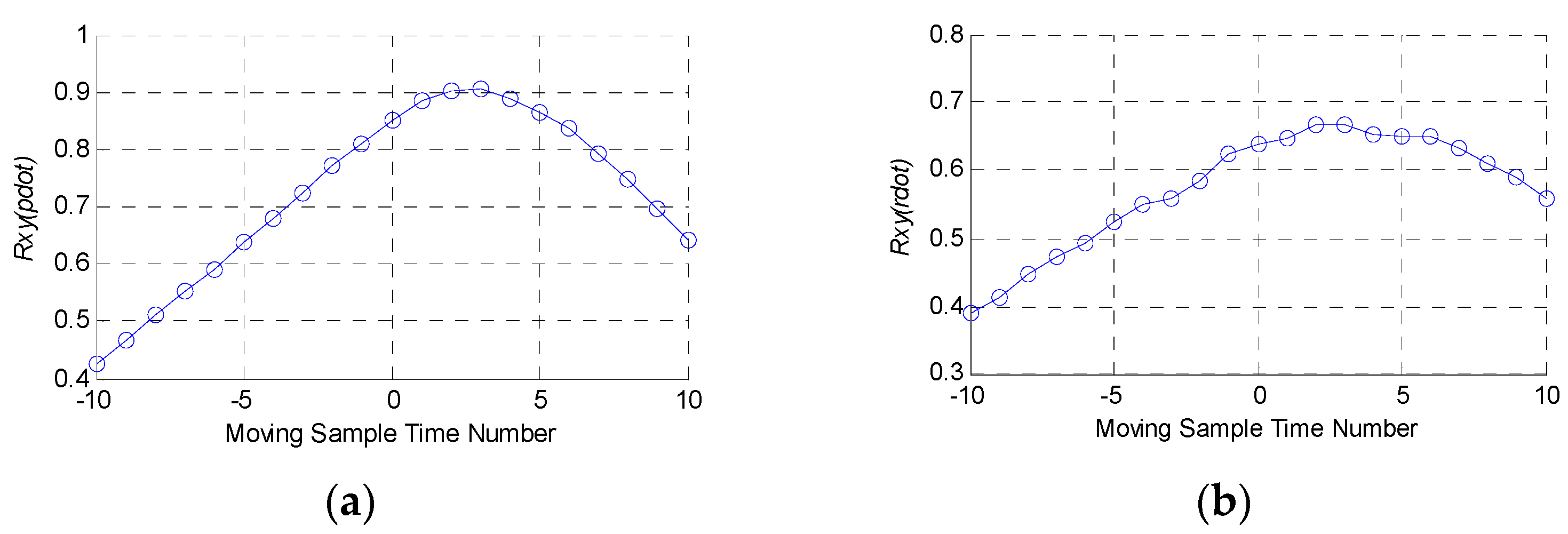
Time delay of the control surface deflection data could be gained with the calculation of the cross-correlation function between AAR of the AVEM and differential angular velocity data. Then, the time-delay calibration of control surface deflection data is carried out;

(3)

The unknown parameters in the generic aerodynamic model are iterated once again with the calibrated control surface deflection data to make the AVEM fit the flight data. The aerodynamic moment coefficient observations calculated using the angular acceleration of the AVEM at this moment could be applied for the identification of aerodynamic derivatives. The flow diagram of the angular acceleration estimation method is shown as Figure 2:

3. Segmented Adaptation Method of Data Segments and Identification Models

3.1. Data Segmentation Method Based on Requirements of Identifiability

The flight test data must meet three requirements to ensure the identifiability of aerodynamic derivatives. The first is that the magnitude of the flight test data must be significantly larger than the error of sensor measurement. The flight data cannot be used for identification when its magnitude is close to the error of sensor measurement [14]. The second is that data cannot be collinear. It is very difficult to obtain unique and definite identification results through conventional identification methods when the data collinearity is obvious, because the models constructed by different parameter combinations can respond similarly to the same input signal. The third is that the magnitude of the aerodynamic force and moment coefficients, generated by variables of motion state and control, must be significantly larger than the measured and estimated observation error. If the magnitudes of the former are close to the observation error, the content of the flight data will be covered by the observation error. It is likely to lead to an ill-conditioned information matrix in identification [13,18]. It contributes to the failure of the identification or the unreliability of identification results.

The identifiability of flight test data cannot be improved effectively through data reconstruction methods, such as compatibility checks and flight path reconstruction. These methods are usually based on the hypothesis that there is no wind [19,20,21,22]. Alternatively, the wind disturbance is estimated as unknown variables. The influence of wind disturbance on the small motion state variables (especially sideslip angle) is more obvious. It is difficult to accurately measure and estimate wind disturbance, making iteration convergence difficult when calculating sideslip angle.

When carrying out aerodynamic parameter identification, the effective content of flight test data will be analyzed quantitatively, and the flight test data will be segmented on the basis of the identifiability of aerodynamic derivatives. The steps are as follows:

(1)

The variance of the observation error is estimated and used as the benchmark for the observation error, the estimation formula is the following:

$${\widehat{\sigma }}^2=\frac{{\displaystyle \sum _{i=1}^N{[z(i)-\widehat{y}(i)]}^2}}{(N-n_p)}$$

(14)

where z is the observation variable, $\widehat{y}$ is the output of the least squares fitting model containing all unknown parameters, N is the data length and n_p is the number of independent variables;

(2)

The data segments whose observation magnitude is 5 times greater than the observation error are selected for identification, on the basis that the magnitude of most data is obviously greater than the sensor measurement error and there is no obvious collinearity;

(3)

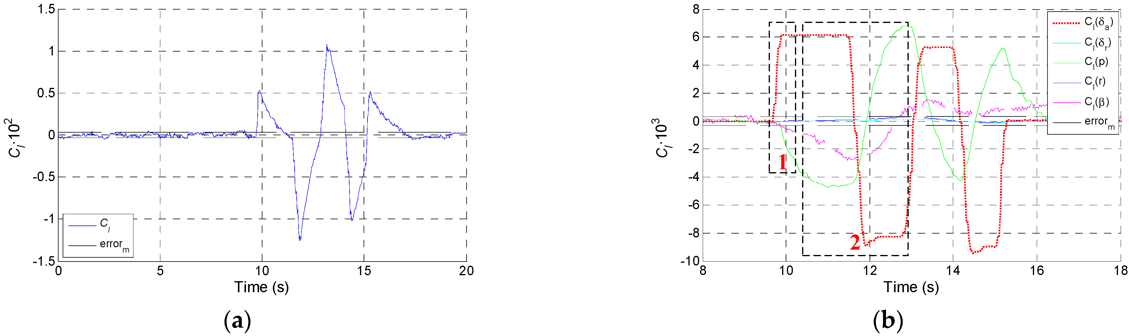
On the basis of data segmentation in the previous steps, the aerodynamic derivatives obtained from wind tunnel tests are used to calculate the magnitude of each component of aerodynamic force and moment coefficients in the motion of aircraft. Further, the data will be segmented according to the components and the magnitude of aerodynamic force or moment coefficient generated by each motion variable and control variable. The components of aerodynamic force and moment within the same data segment should be similar so that identification can be carried out using the same identification model. Aerodynamic force or moment coefficients generated by motion variables and control variables should be significantly greater than the observation errors to reduce its impact on identification results.

3.2. Identification Model Adaptation Method Based on Segmented Flight Test Data

If the identification model containing all the unknown derivatives is directly used in the identification of segmented data, the identification results will not be satisfactory. On the contrary, the accuracy of identification results will be affected negatively with the error contained in the redundant independent variables in the model [1,2]. Therefore, it is necessary to elaborate the optimal identification model for the selected data segment. The aircraft motion variables and control variables in model [1,2] are taken as a set of independent variable candidates, and the identification model structure fitting each data segment is preliminarily determined by the stepwise regression method, which is widely used for the determination of identification model [22,23]. The partial F test is used to determine whether the independent variables have significant contribution to the regression of observation variables under the given significance level (confidence level = 0.05 is adopted in this paper), and then the identification model structure is determined [23,24].

Generally, due to the existence of errors in the aerodynamic derivatives obtained from wind tunnel tests, the identifiability analysis and data segmentation of flight test data with these derivatives are not absolutely good with precision. The identification model structure determined by the stepwise regression method is often not optimal when the segmentation scope of data is not properly selected. Therefore, it is necessary to further tune the data segmentation and corresponding model structure according to the model adaptation evaluation metrics, in order to make the data segment and identification model adapt each other, to reduce the unfitted components in the residual error, and to remove the redundant independent variables in the model. In this paper, the evaluation metrics of model adaptation are goodness of fit (GOF), predicted square error (PSE) and Bayesian information criterion (BIC).

(1)

The fitting evaluation metric of the identification model to the observation variable.

GOF refers to the fitting degree of the identification model to the observation variable and is used as an absolute metric to evaluate the fitting of the model to data.

$$\mathrm{GOF}=1-\frac{{\left(Z-Y\right)}^T\left(Z-Y\right)}{{\left(Z-Z_0\right)}^T\left(Z-Z_0\right)}$$

(15)

where Z is the observation vector composed of observed values of C_Y, C_l and C_n, and Z₀ is the initial value of Z. Y is C_Y, C_l and C_n of the identification model output. The closer GOF is to 1, the better the fitting is. A small GOF indicates that the main content in the observation variable is not fitted by the model, and the identification model does not match the observation variable [23,24].

(2)

The fitting evaluation metric of the identification model structure of side force.

PSE is a widely used statistical metric to determine the model structure, which consists of MSFE and overfitting penalty term [23,24]:

$$\mathrm{PSE}=\mathrm{MSFE}+{\sigma }_{\max }^2\frac{P}{N}$$

(16)

MSFE is mean squared fit error.

$$\mathrm{MSFE}=\frac{1}{N}{\left(\mathrm{Z}-Y\right)}^{\mathrm{T}}\left(Z-Y\right)$$

In Equation (16), constant ${\sigma }_{\max }^2$ is a pre-estimate of the upper bound on the square of the error between the data and the model; P is the number of independent variables in the model, and N is the number of data points. MSFE represents the model fitting characteristics, and ${\sigma }_{\max }^{2}P/N$ is the overfitting penalty term. The overfitting symbolizes that the number of independent variables in the model is more than the independent variables required to fit the observation variable. The side force identification model is optimal in that PSE will increase regardless of whether the independent variable in the model increases or decreases (in general, PSE is a small positive number).

(3)

The fitting evaluation metric of the identification model structure of lateral-directional moment.

In the excitation response of the lateral-directional control surface 3-2-1-1 input, the roll moment is mainly generated by the asymmetric lift force of the wings on both sides, and the yaw moment is mainly generated by the asymmetric side force of the front and rear body and vertical tail of the aircraft. Generally, the magnitude of asymmetric lift force and asymmetric side force is smaller than the side force of the whole aircraft; meanwhile, the length of the moment arm between the asymmetric force and the gravity center is shorter than the wingspan. As a result, the magnitude of C_Y is often larger than C_l and C_n; that is, the orders of magnitude of MSFE of C_l and C_n is lower than C_Y, which may lead to excessive weight of the penalty term for overfitting in PSE. Consequently, it is likely to cause underfitting if PSE is used as a fitting metric of model adaptation [24,25]. Underfitting denotes that the number of independent variables in the model is not enough to fully fit the observation variable, and the model cannot fully describe the data characteristics. The MSFE in BIC is converted into a logarithm to make the weight of MSFE greater when the magnitude of observation is small. The BIC is as follows [24,25]:

$$\mathrm{BIC}(\alpha )=N\ln (\mathrm{MSFE})+P\ln (N)$$

(17)

The first term of Equation (17) is the maximum likelihood function, which is used to evaluate the fitting of the model; the second term is the penalty term for the increase of independent variables in the model. The model with the maximum BIC absolute value is used as the roll and yaw moment identification model (BIC is generally negative).

Fine-tuning the data segment scope and introducing a variable with the greatest contribution to the fitting into the identification model, or removing the variable with the least contribution to the fitting of the observation from the model, is essential for adaptation of identification model structure and data segmentation. The side force identification model structure is determined when GOF is close to 1 and PSE is minimum. The lateral-directional moment identification model structure is determined when GOF is close to 1 and BIC has the maximum absolute value.

To sum up, the process of data segmentation and model adaptation is as follows:

(1)

Flight data is segmented based on requirements of identifiability. Firstly, the observation error is estimated, and the data segments whose observation value is 5 times greater than observation error are selected for identification. Further, the data are segmented according to the components and the magnitude of aerodynamic force and moment coefficients generated by each motion variable and control variable;

(2)

The model structure of each data segment is determined preliminarily through the stepwise regression method. Then, the scope of the data segment and model structure will be fine-tuned to make them adapt each other. The flow diagram of the data segmentation and model adaptation method is shown as Figure 3:

4. Aerodynamic Parameter Identification and Solution Method

4.1. Identification Procedure of Aerodynamic Derivatives

Based on the discussion in the two chapters above, the established identification procedure of 12 lateral-directional aerodynamic derivatives is shown as Figure 4.

As shown in Figure 4, DSMA is the data segmentation and model adaptation method. C_lδa and C_lp are identified through the data segments of the initial stage of the response of the 3-2-1-1 aileron input. C_lδr, C_nδr, C_nβ, C_Yβ and C_Yδr are identified through the data segments of the initial stage of the response of the 3-2-1-1 rudder input. Based on this, C_nr is identified by selecting the data segment with good identifiability of C_nr. Then, the ratio between δ_a, δ_r and β in steady heading sideslip and the identification results of C_lδa and C_lδr are used to solve C_lβ, and the results of C_nδr and C_nβ are used to solve C_nδa. Finally, C_nδa, C_nδr, C_nβ and C_nr are used to identify C_np through data segments with good C_np identifiability in the 3-2-1-1 aileron input response. C_lδr, C_lβ and C_lp are used to identify C_lr through data segments with good C_lr identifiability in the 3-2-1-1 rudder input response.

4.2. Least Squares Mixed Estimation for Step-by-Step Identification

At the initial stage of the aircraft response of aileron and rudder 3-2-1-1 inputs, the control moment is the absolute dominant moment affecting the aircraft motion because other variables are small, except for the control surface deflection angle. Additionally, other weak moments have little influence on the aircraft motion. Therefore, the roll and yaw moment identification model can be simplified as:

$$\{\begin{array}{l}{C}_l=C_{l{\delta }_a}{\delta }_a+\Delta C_l+v_l\\ C_n=C_{n{\delta }_r}{\delta }_r+\Delta C_n+v_n\end{array}$$

(18)

where ΔC_l and ΔC_n represent the moment coefficients with relatively weak influence on aircraft roll and yaw motion, but they are still identifiable. v_l and v_n are the fitting residuals of rolling and yaw moment models, respectively. ΔC_l usually contains lateral static stability moment and rolling damping moment coefficient; v_l usually contains unidentifiable components such as C_l observation error and cross moment coefficient produced by yawing motion. ΔC_n usually contains directional static stability moment; v_n usually contains unidentifiable components such as C_n observation error, yawing damping moment coefficient, and cross moment coefficient produced by rolling motion. The estimation of C_lδa and C_nδr can be completed directly based on identification model (18) through the ordinary least squares method. The general form of the least squares identification model is [1]:

$$\{\begin{array}{l}\mathit{y}=\mathit{X}\mathit{\theta }\\ \mathit{z}=\mathit{X}\mathit{\theta }+\mathit{v}\end{array}$$

(19)

where θ = [θ₀ θ₁…θ_n]^T is the n × 1 aerodynamic derivative vector to be identified; y is the N × 1 aerodynamic force or moment coefficient output vector; z is the N × 1 aerodynamic force or moment coefficient observation vector; X is the N × n independent variable matrix composed of the motion variables, control variables and other parameters of the aircraft; v is the measurement error vector, which meets the white noise hypothesis:

$$E(\mathit{v})=0E(\mathit{v}{\mathit{v}}^T)={\sigma }^2\mathit{I}$$

(20)

The least squares solution of the unknown parameter is

$$\widehat{\theta }={({\mathit{X}}^T\mathit{X})}^{-1}{\mathit{X}}^T\mathit{z}$$

(21)

The covariance of the estimation result is:

$$\mathrm{cov}(\widehat{\theta })={\sigma }^2{({\mathit{X}}^T\mathit{X})}^{-1}$$

(22)

What should not be ignored is that, since v_l and v_n contain unidentifiable components such as cross moment coefficient and yaw damping moment coefficient, their sequences are time-correlated and their mean values are not zero. The magnitude of the unidentifiable terms is small after the accomplishment of data segmentation and model adaptation; that is to say, the unfitted component of the residual is basically in the same order of magnitude as the observation error. Thus, the residual sequence can still be approximately treated as white noise with no obvious impact on the accuracy of least squares estimation results.

In the initial motion stage after the aircraft has been controlled, the control moment is the dominant moment, and the other moment components are small and can be ignored. However, in other stages, the aircraft will also be actuated by damping moment, stability moment and other components. At this moment, the measurement errors of aerodynamic angle, angular velocity and other data will have a significant impact on the fitting. As the dominant aerodynamic force and moment of the aircraft motion change constantly, the impact of measurement errors of each data point on the fitting also changes constantly, so it is difficult to obtain high-consistency identification results by the ordinary least squares method. To obtain more accurate identification results, the least squares mixed estimation method can be used for parameter identification, and the mean and variance of aerodynamic derivatives obtained earlier can be used as prior information to identify other aerodynamic derivatives. For some variables with prior information as constraints in model (19), the constraint form is [1]

$${\mathit{z}}_1={\mathit{X}}_1{\mathit{\theta }}_1+\mathit{\varsigma }$$

(23)

where X₁ is a m × n (m < n) constraint matrix. z₁ is a m × 1 specified observation vector. θ₁ is the subset of θ, which consists of some derivatives which have been identified. ς is a random vector and represents the estimation error of prior information.

$$E(\varsigma )\approx 0,E(\mathit{v}{\varsigma }^{\mathrm{T}})\approx 0,E(\varsigma {\varsigma }^T)\approx {\sigma }^2\mathit{V}$$

(24)

where V is a known matrix, representing the accuracy of prior information. The more accurate the prior information is, the smaller the absolute value of elements in V will be. The mixed model formed after the combination of (19) and (23) is

$$\left[\begin{array}{l}\mathit{z}\\ {\mathit{z}}_1\end{array}\right]=\left[\begin{array}{l}\mathit{X}\\ {\mathit{X}}_1\end{array}\right]\theta +\left[\begin{array}{l}\mathit{v}\\ \mathit{\varsigma }\end{array}\right]$$

(25)

$$E\left\{\left[\begin{array}{l}\mathit{v}\\ \mathit{\varsigma }\end{array}\right]\right\}=0,E\left\{\left[\begin{array}{l}\mathit{v}\\ \mathit{\varsigma }\end{array}\right]{\left[\begin{array}{cc}\mathit{v}& \mathit{\varsigma }\end{array}\right]}^T\right\}={\sigma }^2\left[\begin{array}{l}\begin{array}{cc}\mathit{I}& 0\end{array}\\ \begin{array}{cc}0& \mathit{V}\end{array}\end{array}\right]$$

The least squares solution of the mixed estimation is

$${\widehat{\theta }}_{ME}={\left({\mathit{X}}^T\mathit{X}+{\mathit{X}}_1^T{\mathit{V}}^{-1}{\mathit{X}}_1\right)}^{-1}\left({\mathit{X}}^T\mathit{z}+{\mathit{X}}_1^T{\mathit{V}}^{-1}{\mathit{z}}_1\right)$$

(26)

${\widehat{\theta }}_{ME}$ is the final identification result containing prior information and the derivative to be identified.

5. An Example of Lateral-Directional Aerodynamic Derivative Identification

In this paper, the lateral-directional aerodynamic parameters are identified and validated using the flight test data of a conventional layout twin-engine jet civil aircraft. The aircraft’s reference wing area is 128 m² and its wingspan is 35 m. In order to reduce the impact of the control system on aerodynamic parameter identification in the flight test, the control law outer loop is disconnected, and only the inner-loop yaw damper is retained. The yaw damper deflects the rudder during the response of the 3-2-1-1 aileron input; meanwhile, ailerons do not deflect during the response of the 3-2-1-1 rudder input. The flight test is carried out at an altitude of 4500 m with a speed of 155 m/s. The random error of sensor measurement is described by the root mean square error (RMSE) [14]. The RMSE of angular velocity data is 0.02 °/s. The RMSE of sideslip angle data is 0.025°, the RMSE of acceleration data is 0.004 g, the RMSE of dynamic pressure data is 1 Pa and the RMSE of airspeed data is 0.1 m/s.

5.1. Estimation of Angular Acceleration

The initial values of unknown parameters in model (8) are given in

Table 1. Initial values of unknown parameters in generic aerodynamic moment model.

Cl	Cm		Cn
θ1 = −0.16	θ6 = 0.03	θ7 = −1.49	θ16 = 0.17	θ17 = −0.22
θ2 = −0.46	θ8 = −40.68	θ9 = −2.09	θ18 = −0.47	θ19 = 0.004
θ3 = 0.59	θ10 = −0.5	θ11 = 0	θ20 = −0.19	θ21 = 0
θ4 = −0.086	θ12 = 0	θ13 = 0	θ22 = 0
θ5 = 0.023	θ14 = 0	θ15 = 0

.

The differential data of angular velocity are used as the time reference for synchronizing the control surface deflection data with the angular velocity data. The cross-correlation function values of AAR of the AVEM and differential signals of angular velocity data are shown in the figure below. The values are obtained by moving control surface deflection data different numbers of sampling periods forward and backward.

R_xy of the vertical axis in Figure 5 is the cross-correlation coefficient of x-sequence variables and y-sequence variables in formula (13). In Figure 5a,b, the x sequence is the differential flight test data of roll and yaw angular velocity, respectively. The y sequence is the roll AAR (p_dot) and yaw AAR (r_dot) of the AVEM, respectively. R_xy(p_dot) represents the cross-correlation coefficient between the differential data of roll angular velocity data and the roll AAR of the AVEM. R_xy(r_dot) represents the cross-correlation coefficient between the differential data of yaw angular velocity and yaw AAR of the AVEM. It can be seen from Figure 5 that the cross-correlation function between the angular accelerations of the AVEM and the differential signals of the angular velocity data has the maximum value when the angular acceleration sequence of the AVEM moved forward three sampling periods. Therefore, it can be determined that the time delay of aileron and rudder data is three sampling periods. The aileron and rudder data should be moved forward three sampling periods. After the synchronization calibration, the angular velocity data can be fitted again to obtain the AVEM with higher accuracy. Iteration results of unknown parameters are shown in

Table 2. Iteration results of unknown parameters in generic aerodynamic moment model.

Cl	Cm		Cn
θ1 = −0.18	θ6 = 0.05	θ7 = −1.03	θ16 = 0.11	θ17 = −0.22
θ2 = −0.37	θ8 = 30.29	θ9 = −2.12	θ18 = −0.32	θ19 = 0.51
θ3 = 0.68	θ10 = −80.80	θ11 = −24.49	θ20 = −0.19	θ21 = −0.43
θ4 = −0.078	θ12 = 0.045	θ13 = 5.17	θ22 = 27.5
θ5 = 0.039	θ14 = −0.01	θ15 = 0

.

The 3-2-1-1 aileron input is taken as an example to show the fitting of the AVEM to angular velocity data at this moment, as shown in the Figure 6.

Figure 6 shows that the roll velocity response of the AVEM and the flight test data nearly overlap after time-delay calibration of control surface deflection data. The angular acceleration of the AVEM is used as the estimation of angular acceleration to calculate the observation of moment coefficient.

5.2. The Identification of C_lδa, C_lp

5.2.1. Data Segmentation

Identification analysis and data segmentation are carried out for the flight data of the aircraft’s response to the 3-2-1-1 aileron input. First, the observation C_l of the rolling moment coefficient of the aircraft is calculated by Equation (2) based on the estimated angular acceleration. Then, the variation of each rolling moment component is calculated by Equation (1) based on both aerodynamic derivatives (C_lδa, C_lδr, C_lβ, C_lp and C_lr) gained from wind tunnel tests and the flight test data such as aileron deflection, roll angle velocity and sideslip angle, as shown in Figure 7.

The variance of C_l observation error is estimated by Equation (14) firstly. The standard deviation of the estimation error is about 3.5 × 10⁻⁴, and ±3.5 × 10⁻⁴ is taken as the C_l observation error bound (error_m in the Figure 7b). As can be seen from Figure 7a, the magnitude of C_l from 9.5 to 17 s is significantly greater than the observation error. Therefore, 9.5~17 s data are preliminarily selected for parameter identification.

Based on this, data are further segmented according to the variation of moment components, as shown in Figure 7b. The maximum absolute value of aileron rolling moment coefficient C_l(δ_a) is 6.2 × 10⁻³ and the maximum absolute value of roll damping moment coefficient C_l(p) is 2.4 × 10⁻³ within the range of 9.5~10.2 s, which are both larger than 5 times C_l errors. The maximum absolute values of lateral static stability moment coefficient C_l(β), control moment coefficient of rudder C_l(δ_r) and cross moment coefficient produced by yaw motion C_l(r) are 1.3 × 10⁻⁴, 2.0 × 10⁻⁴ and 8.2 × 10⁻⁵, respectively, which are all smaller than C_l errors. In the range of 9.5~10.2 s, C_l(δ_a) plays a dominant role in the rolling motion, followed by C_l(p). C_l(β), C_l(r) and C_l(δ_r) have almost no influence on the rolling motion, which is beneficial to the identification of C_lδa. The data segment is numbered 1 for the identification of C_lδa, and its suffix is I. There are 22 data points in this data segment.

In the time scope of 10.4~13.0 s, the maximum absolute values of C_l(δ_a), C_l(p) and C_l(β) are 8.9 × 10⁻³, 6.8 × 10⁻³ and 2.3 × 10⁻³, respectively, which are all much larger than 5 times C_l errors. The maximum absolute values of C_l(δ_r) and C_l(r) are 2.0 × 10⁻⁴ and 1.0 × 10⁻⁴, respectively, which are both smaller than C_l errors. In this data segment, C_lδa, C_lp and C_lβ are identifiable. C_l(p) is one of the dominant moments of rolling motion, and this data segment is beneficial to C_lp identification. This data segment is numbered 2, and its suffix is II. There are 86 data points in this data segment. The identification of C_lp is carried out with this data segment by using C_lδa identification results as prior information.

Compared with C_l(δ_a) and C_l(p), C_l(β) has weaker influence on rolling motion, and there are less data available for C_lβ identification in the data of whole response. Considering the poor measurement accuracy of sideslip angle, the identifiability of C_lβ in the data reduces, making it difficult to obtain reliable identification results. Both C_l(δ_r) and C_l(r) in the whole response data are smaller than C_l error, indicating that the information of C_l(δ_r) and C_l(r) in the 3-2-1-1 aileron input response data would be covered by C_l error. A reliable C_lδr and C_lr cannot be obtained. In other words, the contribution of C_l(δ_r) and C_l(r) to the C_l fitting should be treated as colored noise during identification.

From the analysis above, it can be seen that, in the data of response to the 3-2-1-1 aileron input shown in Figure 7b, the identifiability of C_lδa and C_lp are good, C_lβ is poor, and C_lr and C_lδr are unidentifiable. Data segments 1 and 2 have different identifiability; thus, they need to be identified by different identification models. In view of the fact that C_lδa and C_lp can be obtained through the data segments 1 and 2, at the same time, C_lβ, C_lr and C_lδr cannot be accurately identified through the data of any parts in the 3-2-1-1 aileron input response, making data segmentation meaningless. The identification of C_lβ, C_lr and C_lδr will be carried out in the following descriptions with the data of the 3-2-1-1 rudder input and SHSS.

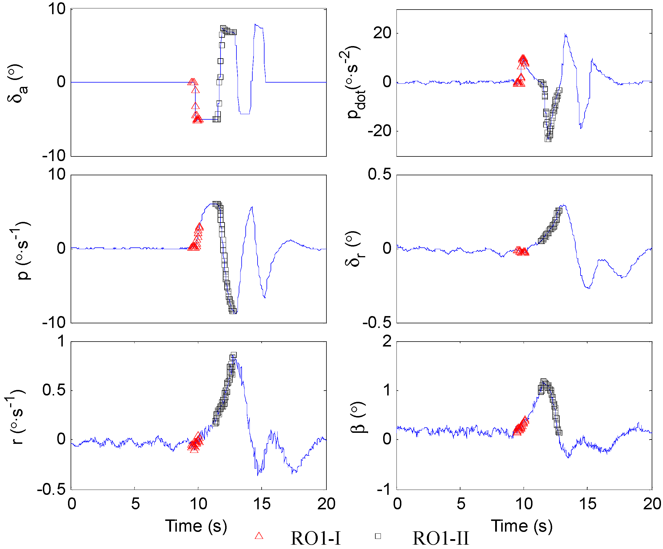
5.2.2. The Adaptation of Data Segments and Identification Models

After the data are segmented preliminarily, stepwise regression is used to determine the identification model structure corresponding to each data segment. At the confidence level of α = 0.05, δ_a and $\overline{p}$ in data segment 1 have significant contribution to C_l regression, and the identification model structure of data segment 1 is as follows:

$$C_l=C_{l{\delta }_a}{\delta }_a+C_{lp}\overline{p}+v$$

(27)

where v is the C_l fitting residual, including components such as rudder rolling control moment coefficient C_l(δ_r) and cross moment coefficient produced by yaw C_l(r). In this paper, all of the fitting residuals v in different identification models contain unfitted components, whose sequences are time-dependent and mean values are not zero. This will not be repeatedly illustrated below. The identification model structure of data segment 2 can also be determined by stepwise regression, and the model structure is as follows:

$$C_l={\tilde{C}}_{l{\delta }_a}{\delta }_a+C_{lp}\overline{p}+C_{l\beta }\beta +v$$

(28)

where, the derivative with “~” overline means the obtained identification results are used as prior information in identification, the same as below. The scope of data segment and model structure are tuned to make the absolute value of BIC maximized when GOF is closest to 1. Finally, the time scope of segment I is 9.5~10.2 s, denoted as RO1_I, and the corresponding model structure is (27). At this time, The GOF is 0.995, indicating that the data can almost be completely fitted by the model. The BIC of model (27) for RO1_I is −381. β is the variable having the most significant contribution to C_l fitting among the independent variables not introduced into model (27). After its introduction into model (27), BIC is −379. p is a variable with relatively weak contribution to C_l fitting in model (27), and BIC is −349 after it is removed. The absolute value of BIC of the original model (27) is the largest, and the RO1_I data segment matches model (27).

The scope of segment II is determined to be 11.6–12.8 s using the same method, and is denoted as RO1_II with the suitable model (28). There are 40 data points in the segment. GOF is 0.998 and BIC is −704. The segmented scopes of RO1_I and RO1_II are shown in Figure 8.

5.2.3. Parameter Estimation

C_lδa is estimated through model (27) and RO1_I by the ordinary least squares method. C_lδa is −1.15 × 10⁻³, and its variance is 7.56 × 10⁻¹⁰; C_lp is −6.13 × 10⁻³, and its variance is 4.24 × 10⁻⁷. The estimation of C_l fitting error of the identification model is 3.27 × 10⁻⁴; the fitting error estimated by Equation (14) is 2.59 × 10⁻⁴, and the difference between them is small. It indicates that the identification results for RO1_I using simplified model (27) is similar to those gained using the model containing all independent variables.

The identification results of C_lδa obtained by the ordinary least squares method are substituted into Equation (25) as prior information, and the least squares mixed estimator is used to estimate C_lp through model (28) and RO1_II. C_lp is −6.17 × 10⁻³, and its variance is 3.96 × 10⁻⁸; C_lβ is −3.24 × 10⁻³, and its variance is 1.80 × 10⁻⁹. The estimation of C_l fitting error $\widehat{\sigma }$ is 3.53 × 10⁻⁴. The fitting error estimated by Equation (14) is 2.45 × 10⁻⁴. The slight difference between the two fitting errors indicates the identification results obtained from RO1_II, using the simplified model (28) and prior information of C_lδa, are similar to the results obtained through the model containing all independent variables.

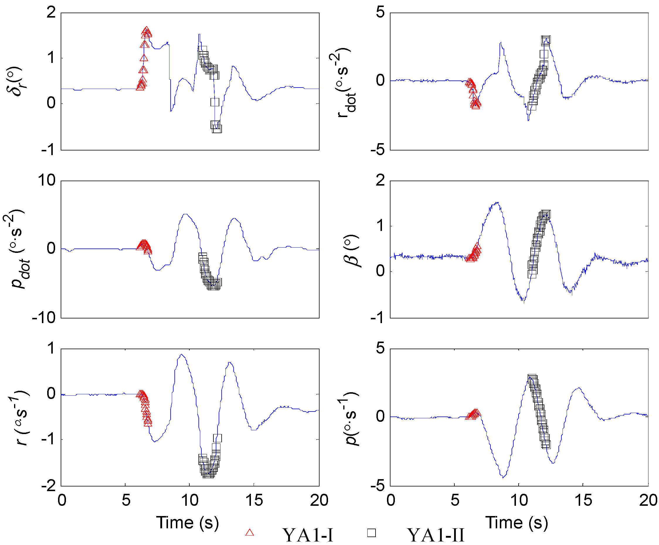
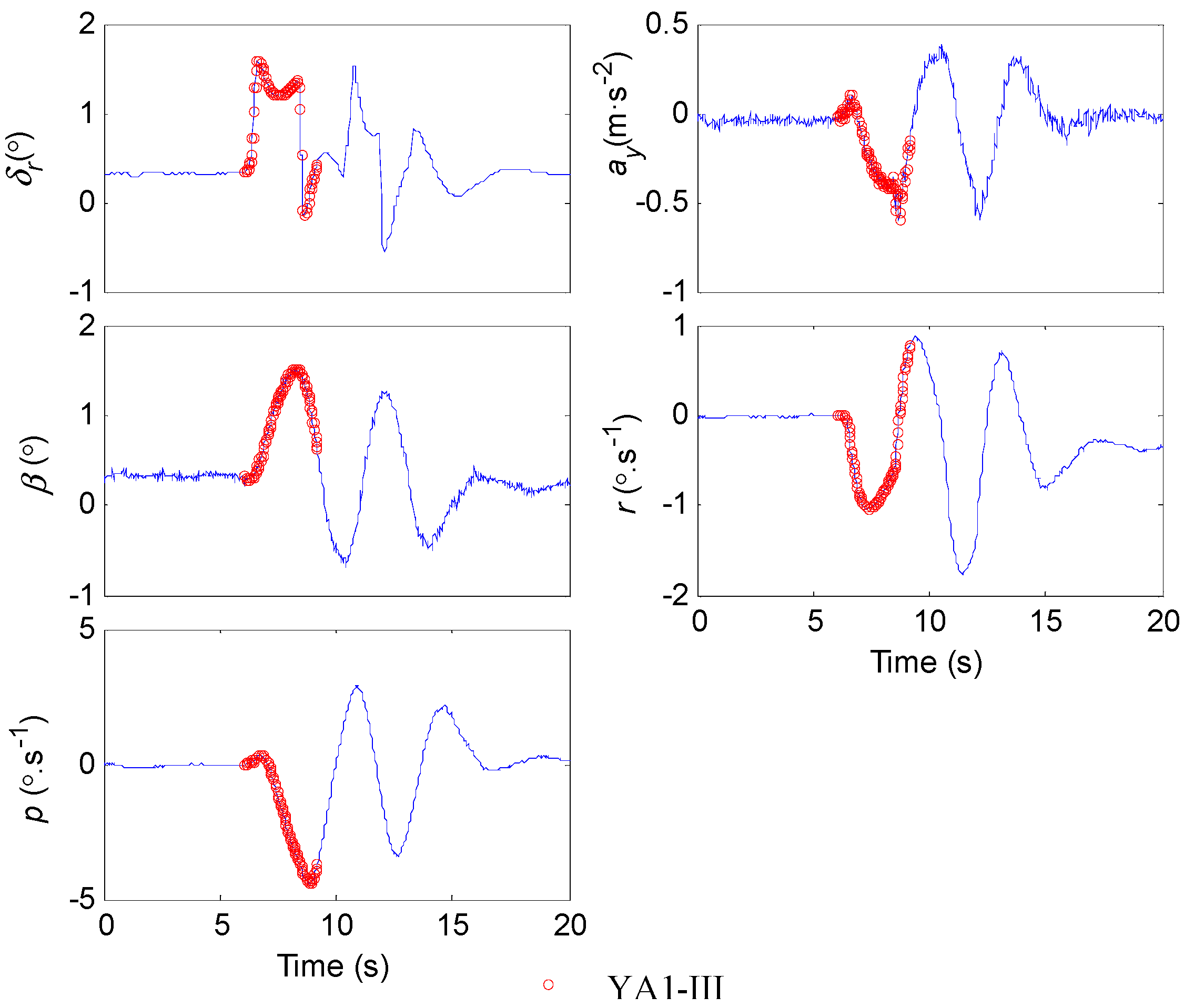
5.3. The Identification of C_nδr, C_lδr, C_nβ, C_nr, C_Yδr and C_Yβ

The process of data segmentation and model adaptation using the data of the 3-2-1-1 rudder input response is similar to that mentioned above, which will not be described here. The results of data segmentation, model adaptation and identification of aerodynamic derivatives are directly presented here. The data segments used for identification of C_nδr, C_lδr and C_nβ are denoted as YA1-I, and the data segments used for C_nr identification are denoted as YA1-II, as shown in Figure 9.

The rolling and yaw moment identification model adapting data segments YA1 is as follows:

$$\{\begin{array}{l}{C}_l=C_{l\beta }\beta +C_{l{\delta }_r}{\delta }_r+v\\ C_n=C_{n\beta }\beta +C_{n{\delta }_r}{\delta }_r+v\end{array}$$

(29)

The yaw moment identification model adapting data segments YA1-II is:

$$C_n={\tilde{C}}_{n\beta }\beta +{\tilde{C}}_{n{\delta }_r}{\delta }_r+C_{np}\overline{p}+C_{nr}\overline{r}+v$$

(30)

The results obtained through YA1-I and model (29) are as follows: C_nδr is −3.13 × 10⁻³; C_nβ is 3.12 × 10⁻³; C_lδr is 0.90 × 10⁻³. Based on the identification results of C_nδr and C_nβ, C_nr obtained through YA1-II and model (30) is −6.53 × 10⁻³.

It should be noted that C_lβ and C_np will be solved and identified through the steps in Section 5.4 according to the identification procedure in Figure 4. C_lβ in model (29) and C_np in model (30) are to ensure the model can fully fit data segments with no identification of their values. Thus, specific identification results are not given here.

The estimated error of C_Y is about 2.2 × 10⁻³ according to Equation (14). The maximum values of C_Y(δ_r) and C_Y(β) are about 1.5 × 10⁻² and 3.0 × 10⁻², respectively, which are more than 5 times larger than the errors of C_Y. Therefore, C_Yδr and C_Yβ can be identified. The data segments used for identification of C_Yδr and C_Yβ are denoted as YA1-III, as shown in Figure 10.

The side force identification model adapting the data segments YA1-III is:

$$C_Y=C_{Y\beta }\beta +C_{Y{\delta }_r}{\delta }_r+v$$

(31)

The identification results of C_Yδr and C_Yβ, obtained through YA1-III and model (31), are 7.83 × 10⁻³ and −2.05 × 10⁻², respectively.

5.4. Solution of C_lβ and C_nδa

The flight data of steady heading sideslip do not need to be segmented, since each motion state variable during trim flight could be regarded as stable. The flight test data under trim state are shown below.

In Figure 11, ailerons, rudder, lateral acceleration and sideslip angle all show obvious ladder pattern characteristics. In order to reduce the disturbance of measurement error on the trim, the mean value of data within every 5 s is used as the value of the data. The relationship between sideslip angle and rudder deflection in steady heading sideslip is obtained by linear regression. The ratio of sideslip angle, rudder deflection angle and aileron deflection angle is 1:0.926:−2.338. The ratio is relatively stable and accurate and is used for the identification and solution of subsequent parameters as prior information. With the constraint of steady heading sideslip, as well as the obtained identification results of C_lδa and C_lδr, C_lβ solved by Equation (7) is −3.52 × 10⁻³. C_nδa solved by Equation (7) is 0.09 × 10⁻³ using the identification results of C_nδr and C_nβ and the steady heading sideslip constraint.

5.5. Identification of Cross Derivatives

C_lδa, C_lp and C_lβ are identified and solved by the data of the 3-2-1-1 aileron input and steady heading sideslip. C_nβ, C_nδr, C_nδa, C_nr and C_lδr are identified and solved by the data of the 3-2-1-1 rudder input. These results are used as prior information for cross derivative identification. The response data segments of the 3-2-1-1 aileron input used for C_np identification are denoted as RO1-III, as shown in Figure 12.

The yaw cross derivative identification model adapting the data segments RO1-III is:

$$C_n={\tilde{C}}_{n\beta }\beta +{\tilde{C}}_{n{\delta }_a}{\delta }_a+{\tilde{C}}_{nr}\overline{r}+({\tilde{C}}_{n{\delta }_r}{\delta }_r)+C_{np}\overline{p}+v$$

(32)

The identification result of C_np is −1.70 × 10⁻³. The data segmentation and model adaptation processes of C_lr identification are similar to those of C_np, which will not be elaborated here. The identification result of C_lr obtained through the response data of the 3-2-1-1 rudder input is 3.34 × 10⁻³.

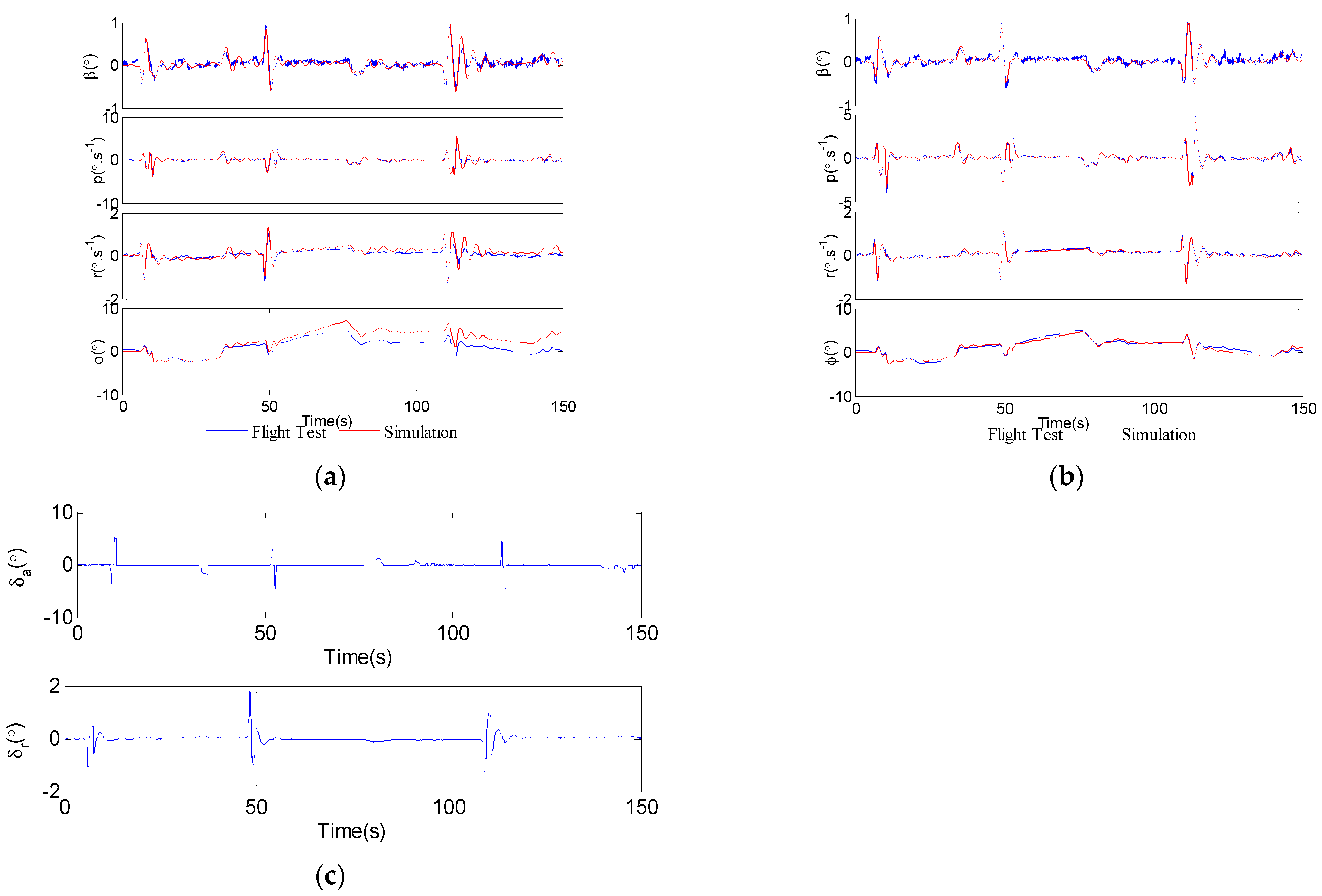
6. Validation of the Identification Results

6.1. Comparison and Analysis of Identification Results

The identification results gained by the conventional MLE method are presented here to make comparison with the DSMA method in terms of consistency and accuracy of the identification results. Unlike the data required in DSMA method, the MLE method requires continuous data. As an excitation signal widely adopted in MLE identification, a combined aileron and rudder doublet signal input is used for obtaining continuous flight test data. The flight test data used for comparison of the two different identification methods are obtained at the same altitude and Mach number. The four groups of combined aileron and rudder doublet input response data are denoted as AR1, AR2, AR3 and AR4. AR1 is shown in Figure 13.

Figure 13 shows that the deflection amplitudes of rudder and aileron in the combined doublet input are similar to deflection amplitudes in the 3-2-1-1 aileron and rudder inputs, which can fully excite the lateral-directional motion and produce obvious roll, yaw angular velocity and lateral acceleration. The four groups of response data of the 3-2-1-1 rudder input are denoted as YA1, YA2, YA3 and YA4. The four groups of response data of the 3-2-1-1 aileron input are denoted as RO1, RO2, RO3 and RO4. Identification results of aerodynamic derivatives are shown in

Table 3. Identification results of aerodynamic derivatives.

The Number of Dataset	RO1 + YA1	AR1	RO2 + YA2	AR2	RO3 + YA3	AR3	RO4 + YA4	AR4
Estimation Method	DSMA (×10−3/°)	MLE (×10−3/°)	DSMA (×10−3/°)	MLE (×10−3/°)	DSMA (×10−3/°)	MLE (×10−3/°)	DSMA (×10−3/°)	MLE (×10−3/°)
CYδr	7.83	7.42	7.52	8.31	7.77	7.68	7.82	8.82
CYβ	−20.5	−21.9	−19.8	−24.3	−20.8	−21.9	−20.3	−20.4
Clδa	−1.15	−1.33	−1.17	−1.38	−1.11	−1.36	−1.19	−1.24
Clδr	0.90	0.89	0.93	0.84	0.98	0.77	0.90	0.97
Clβ	−3.52	−3.69	−3.59	−4.83	−3.44	−3.53	−3.61	−4.66
Clp	−6.17	−6.47	−6.17	−7.17	−6.14	−6.14	−6.14	−7.39
Clr	3.34	4.88	4.28	1.82	3.44	4.37	2.76	4.91
Cnδr	−3.13	−3.31	−2.99	−3.41	−3.12	−3.44	−3.11	−3.45
Cnδa	0.09	0.06	0.16	−0.17	0.11	−0.05	0.04	−0.04
Cnβ	3.12	3.47	3.15	2.62	3.14	3.14	2.98	3.02
Cnp	−1.70	−2.55	−1.53	−3.61	−1.80	−2.74	−1.51	−2.53
Cnr	−6.53	−2.73	−6.41	−4.33	−6.58	−5.72	−6.50	−1.25

.

As can be seen from Table 3, compared with the conventional MLE method, the consistency of results obtained by the DSMA method is significantly improved. The dispersion coefficient (the ratio of standard deviation to mean [25,26]) is used to quantitatively analyze the consistency of identification results. The absolute values of the dispersion coefficient obtained through the two methods are shown in Figure 14.

As can be seen from Figure 14 and Table 3, for C_Yβ, C_Yδr, C_lδa, C_lδr, C_lβ, C_lp, C_nδr, C_nβ and C_np with significant contribution to aircraft motion in the excitation response, the absolute values of dispersion coefficients obtained by DSMA and MLE are small. For example, the absolute values of dispersion coefficients of C_lδa obtained by DSMA and MLE are 3.0% and 4.7%, respectively, and the distribution intervals of absolute values are 1.11 × 10⁻³~1.19 × 10⁻³ and 1.24 × 10⁻³~1.38 × 10⁻³, respectively. The absolute values of dispersion coefficients of C_nβ obtained by DSMA and MLE are 2.6% and 11.5%, respectively, and the distribution intervals of absolute values are 2.98 × 10⁻³~3.15 × 10⁻³ and 2.62 × 10⁻³~3.47 × 10⁻³, respectively. Compared with the MLE method, the distribution interval of DSMA results is more concentrated, and the consistency of the results is higher.

For C_lr, C_nδa and C_nr with relatively slight contribution to aircraft motion in the excitation response, the identification results are less consistent. The distribution intervals of absolute value of MLE identification results of the three derivatives are 1.82 × 10⁻³~4.91 × 10⁻³, 0.04 × 10⁻³~0.17 × 10⁻³ and 1.25 × 10⁻³~5.72 × 10⁻³, respectively, and the corresponding dispersion coefficients are 37%, 188% and 55%, respectively. The consistency of the results is poor. The absolute value distribution intervals of DSMA identification results of the three derivatives are 2.76 × 10⁻³~4.28 × 10⁻³, 0.04 × 10⁻³~0.16 × 10⁻³ and 6.41 × 10⁻³~6.58 × 10⁻³, respectively, and the corresponding dispersion coefficients are 18%, 50% and 2%, respectively. The dispersion degree of the identification results obtained by DSMA is significantly lower than that of MLE, and the consistency of the results is higher.

Since the flight dynamics model of the aircraft has errors, and the data measurement noise is, in fact, not white noise, there are errors in the optimization constraint index established with the similarity between the aircraft motion response and flight test data. This results in inconsistent identification results obtained by using different data. The impact of constraint index error will be reduced by selecting data segments with a larger magnitude of the variable corresponding to the derivative to be identified, and by introducing trim results of steady heading sideslip and accurate identification results as prior information. Further, the accuracy and consistency of identification results are improved effectively.

6.2. Validation of the Identification Results

The lateral-directional small-disturbance linearized motion model of aircraft is established by the aerodynamic derivative identification results in Table 3 [26]. The identification results are comprehensively validated by comparing the motion model responses and flight test data with the same control input. The lateral-directional small-disturbance linearized motion model of aircraft is as follows:

$$\dot{x}=Ax+Bu$$

(33)

$$A=\left[\begin{array}{cccc}{\overline{Y}}_{\beta }& {\alpha }_{*}+{\overline{Y}}_p& {\overline{Y}}_r-1& g\cos {\theta }_{*}/V_{*}\\ {\overline{L}}_{\beta }& {\overline{L}}_p& {\overline{L}}_r& 0\\ {\overline{N}}_{\beta }& {\overline{N}}_p& {\overline{N}}_r& 0\\ 0& 1& \tan {\theta }_{*}& 0\end{array}\right]$$

(34)

$$x={\left[\begin{array}{cccc}\Delta \beta & \Delta p& \Delta r& \Delta \varphi \end{array}\right]}^T$$

(35)

$$B={\left[\begin{array}{cccc}\begin{array}{l}0\\ {\overline{Y}}_{{\delta }_r}\end{array}& \begin{array}{l}{\overline{L}}_{{\delta }_a}\\ {\overline{L}}_{{\delta }_r}\end{array}& \begin{array}{l}{\overline{N}}_{{\delta }_a}\\ {\overline{N}}_{{\delta }_r}\end{array}& \begin{array}{l}0\\ 0\end{array}\end{array}\right]}^T$$

(36)

$$u={\left[\begin{array}{cc}\Delta {\delta }_a& \Delta {\delta }_r\end{array}\right]}^T$$

(37)

The symbols with * in the Equation (34) indicate that they are the base value of the trim flight. The flight test data with aileron and rudder inputs are selected to validate the identification results. Aileron and rudder deflection data are taken as the input of the linearized model. The comparisons between motion model response and flight test data are shown in Figure 15.

Figure 15 shows that the linearized model established on the basis of DSMA results fits flight test data well, and the model established on the basis of MLE results basically fits the flight test data in the first 50 s of simulation, and the errors of yaw velocity and roll angle response of the model increase significantly after 50 s of the simulation. This indicates the identification of derivatives with significant contribution to aircraft motion in MLE results is relatively accurate, while the identification accuracy of derivatives with slight contribution to aircraft motion is poor. It can be further illustrated with Figure 15a that significant differences between model response and flight test data emerge after 50 s of simulation. The GOF of response of the aircraft linearization model, reconstructed through identification derivatives obtained by different methods, to flight test data is shown in

Table 4. GOF of different linearization models of aircraft motion to flight test data.

GOF	β	p	r	ϕ
DSMA	0.8638	0.9207	0.9260	0.9494
MLE	0.6808	0.7350	0.5454	0.3627

.

The GOF values of p, r, and ϕ response of the linearized model to the flight test data are all greater than 0.92, except that the GOF of β is slightly lower at 0.86, caused by large measurement noise and error. This GOF is similar to the fitting results achieved by the accurate lateral-directional dynamics model finally obtained in reference [24]. It indicates that the linearized aircraft motion model reconstructed with the lateral-directional aerodynamic parameter identification results obtained by DSMA can fit the flight test data well, and the identification results are accurate and reliable. The GOF of β, p, r, and ϕ response of the linearized model reconstructed using the MLE identification results to the flight test data is 0.68, 0.74, 0.55 and 0.36, respectively. They are obviously smaller than the GOF gained from the model based on DSMA results, which also indicates that the accuracy of identification results based on MLE is relatively low.

Contrast of the two methods’ results show that selecting valid data with large magnitude through data segmentation and introducing more accurate identification results of derivatives as a priori restraints can effectively improve the identification accuracy of the aerodynamic derivatives. Especially for derivatives such as C_lr and C_nδa with small absolute value and slight contribution to aircraft motion, the identification accuracy has a more significant improvement.

7. Conclusions

(1)

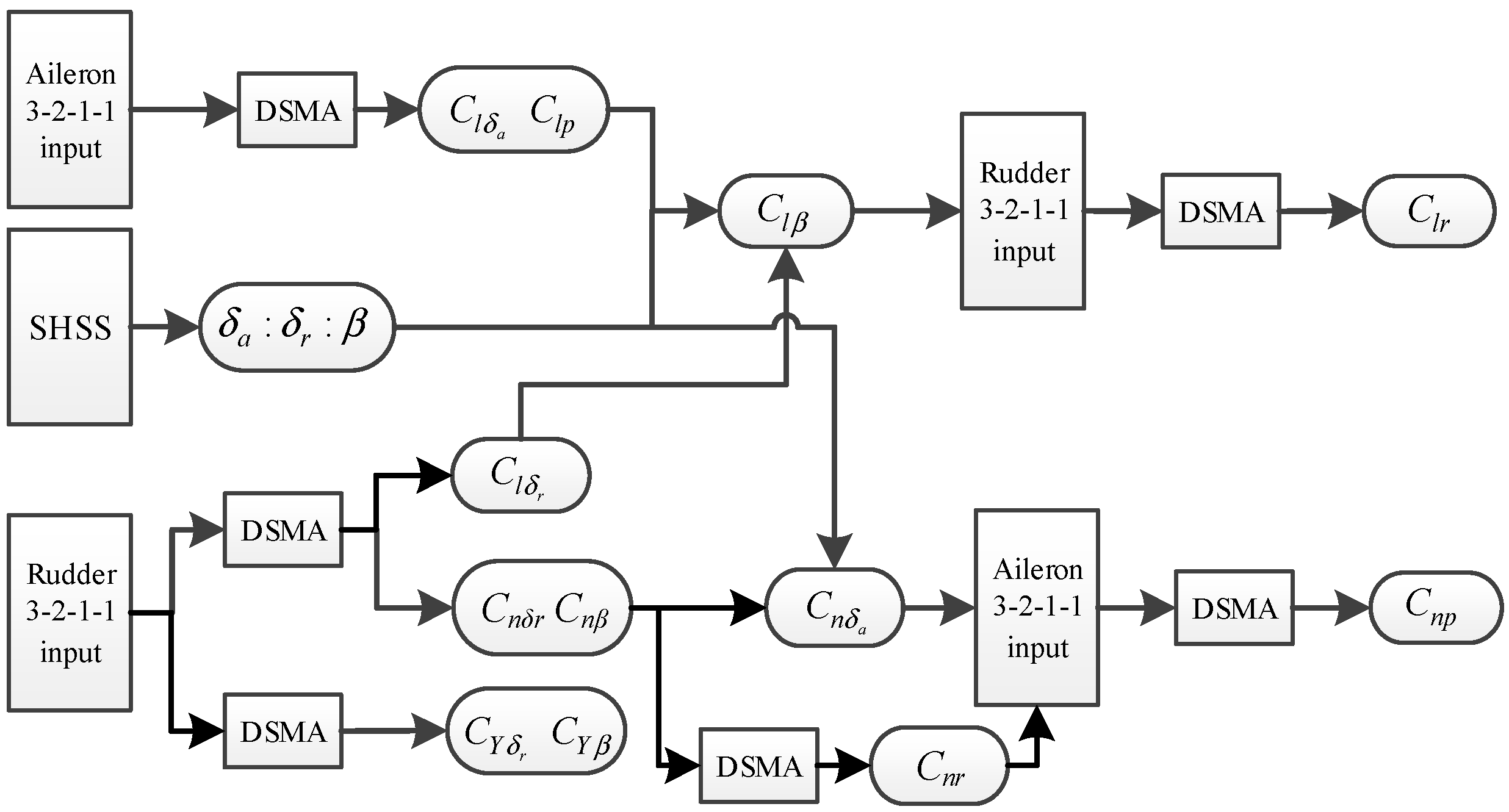
The step-by-step lateral-directional aerodynamic parameter identification procedure is established. First, C_lδa and C_lp are identified by the 3-2-1-1 aileron input; at the same time, C_Yδr, C_Yβ, C_nδr, C_nβ, C_nr and C_lδr are identified by the 3-2-1-1 rudder input. Next, C_lβ and C_nδa are solved through the ratio between sideslip angle, aileron deflection angle and rudder deflection angle in steady heading sideslip. Finally, the identification results gained in the steps above are used as prior constraints for the identification of cross derivative C_np and C_lr.

(2)

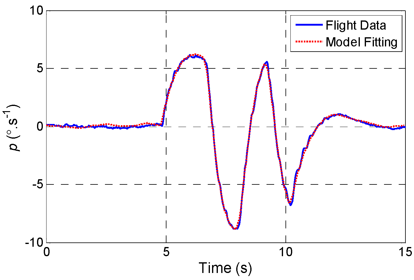
The angular acceleration estimation method based on the angular velocity equivalent model is established. Firstly, an angular velocity equivalent model is established based on the generic aerodynamic moment model and the rotational dynamics equations of aircraft, and the unknown parameters in the model are iterated to make the angular velocity response of the model fit the angular velocity flight data. Then, the time delay between angular velocity data and control surface deflection data is calibrated by using the cross-correlation function between the angular acceleration response of the angular velocity equivalent model and the differential signal of angular velocity data. Finally, the unknown parameters are iterated once again to fit angular velocity data using the calibrated control surface deflection data, and the angular acceleration of the equivalent model at this moment is used as the estimated angular acceleration for aerodynamic parameter identification when conducting flight tests.

(3)

An aerodynamic parameter identification method using segmented adaptation of identification model and flight test data is established. First, the flight test data is segmented preliminarily according to the components as well as the magnitude of aerodynamic force and moment coefficients generated by each variable. Secondly, the scope of data segmentation and the structure of the identification model is determined by stepwise regression and model-fitting metrics combination. Thirdly, the aerodynamic derivative is estimated in stages through the ordinary least squares method and least squares mixed estimator according to the established identification and solving procedure, and C_lβ and C_nδa are solved by using the constraint of steady heading sideslip and the accurate prior identification results.

(4)

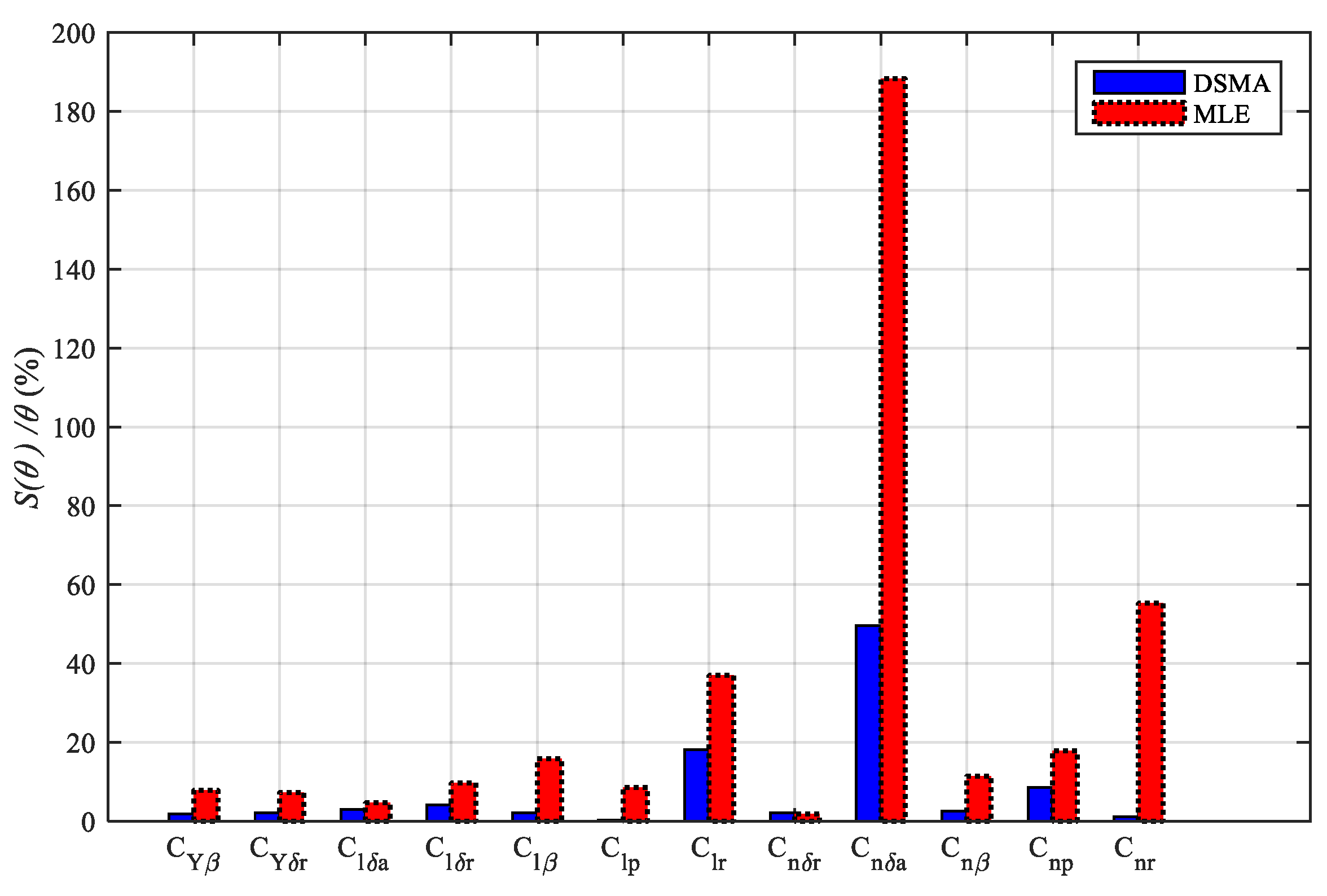
The identification and validation of lateral-directional aerodynamic derivatives are carried out with the DSMA identification method and the conventional MLE identification method. Compared with the conventional MLE method, the lateral-directional aerodynamic derivatives obtained by the DSMA identification method have a higher accuracy and consistency because valid data segments with good identifiability are selected and the obtained accurate identification results and steady heading sideslip trim results are used as prior constraints. Especially for derivatives with small absolute value and slight contribution to aircraft motion, the improvement of identification accuracy is more significant.

The flight test scheme proposed in this paper is simple and can be easily operated by pilots. The identification algorithm of the identification method is also simple and practical, and the results are reliable.

References

1. Klein, V.; Morelli, E.A. Regression Methods. In Aircraft System Identification—Theory and Practice; AIAA Education Series; AIAA: Reston, VA, USA, 2006; pp. 95–180. [Google Scholar]
2. Strutz, T. Uncertainty of Results. In Data Fitting and Uncertainty: A Practical Introduction to Weighted Least Squares and Beyond; Vieweg + Teubner Verlag: Wiesbaden, Germany, 2011; pp. 105–123. [Google Scholar]
3. Liu, S.F.; Luo, Z.; Moszczynski, G.; Grant, P.R. Parameter Estimation for Extending Flight Models into Post-Stall Regime—Invited. In Proceedings of the AIAA Atmospheric Flight Mechanics Conference, San Diego, CA, USA, 4–8 January 2016. [Google Scholar]
4. Saderla, S.; Kim, Y.; Ghosh, A.K. Online system identification of mini cropped delta UAVs using flight test methods. Aerosp. Sci. Technol. 2018, 80, 337–353. [Google Scholar] [CrossRef]
5. Zanette, J.V.; Almeida, F.D. RealSysId: A software tool for real-time aircraft model structure selection and parameter estimation. Aerosp. Sci. Technol. 2016, 54, 302–311. [Google Scholar] [CrossRef]
6. Federal Aviation Administration (2018). Full Flight Simulator (FFS) Objective Tests QPS REQUIREMENTS. In CFR Part 60, Flight Simulation Training Device Initial and Continuing Qualification; USA. 2016; pp. 97–98. Available online: https://www.ecfr.gov/current/title-14/chapter-I/subchapter-D/part-60 (accessed on 10 June 2022).
7. Sousa, M.S.; Paula, A.A. Matching of Aerodynamic databank with Flight test data-Latero-directional Dynamics. In Proceedings of the AIAA Modeling and Simulation Technologies Conference, Grapevine, TX, USA, 9–13 January 2017. [Google Scholar]
8. Morelli, E.A.; Klein, V. Application of System Identification to Aircraft at NASA Langley Research Center. J. Aircr. 2005, 42, 12–25. [Google Scholar] [CrossRef]
9. Sieberling, S.; Chu, Q.P.; Mulder, J.A. Robust Flight Control Using Incremental Nonlinear Dynamic Inversion and Angular Acceleration Prediction. J. Guid. Control Dyn. 2010, 33, 1732–1742. [Google Scholar] [CrossRef]
10. Jatiningrum, D.; Lu, P.; Chu, Q.P.; Mulder, M. Development of a New Method for Calibrating an Angular Accelerometer Using a Calibration Table. In Proceedings of the AIAA Guidance, Navigation, and Control Conference, Kissimmee, FL, USA, 5–9 January 2015. [Google Scholar]
11. Levant, A. Robust Exact Differentiation via Sliding Mode Technique. Automatica 1998, 34, 379–384. [Google Scholar] [CrossRef]
12. Nicolosi, F.; Marco, A.D.; Sabetta, V.; Vecchia, P.D. Roll performance assessment of a light aircraft: Flight simulations and flight tests. Aerosp. Sci. Technol. 2018, 76, 471–483. [Google Scholar] [CrossRef]
13. Morelli, E.A. Global nonlinear aerodynamic modeling using multivariate orthogonal functions. J. Aircr. 1995, 32, 270–277. [Google Scholar] [CrossRef]
14. Morelli, E.A.; Cunningham, K.; Hill, M.A. Global Aerodynamic Modeling for Stall/Upset Recovery Training Using Efficient Piloted Flight Test Techniques. In Proceedings of the AIAA Modeling and Simulation Technologies Conference, Boston, MA, USA, 19–22 August 2013. [Google Scholar]
15. Grauer, J.A.; Morelli, E.A. Generic Global Aerodynamic Model for Aircraft. J. Aircr. 2015, 52, 13–20. [Google Scholar] [CrossRef]
16. Williamson, W.E.; Mcdowell, J.L. Instrument modeling for aerodynamic coefficient identification from flight test data. J. Guid. Control Dyn. 2015, 3, 275–279. [Google Scholar] [CrossRef]
17. Dang, X.W.; Tang, P. Incremental nonlinear dynamic inversion control and flight test based on angular acceleration estimation. Acta Aeronaut. Astronaut. Sin. 2020, 41, 323534. [Google Scholar]
18. Grauer, J.A. Real-Time Data-Compatibility Analysis Using Output-Error Parameter Estimation. J. Aircr. 2015, 52, 940–947. [Google Scholar] [CrossRef]
19. Morelli, E.A. Real-Time Aerodynamic Parameter Estimation Without Air Flow Angle Measurements. J. Aircr. 2012, 49, 1064–1074. [Google Scholar] [CrossRef]
20. Chowdhary, G.; Jategaonkar, R. Aerodynamic parameter estimation from flight data applying extended and unscented Kalman filter. Aerosp. Sci. Technol. 2010, 14, 106–117. [Google Scholar] [CrossRef]
21. Oliveira, J.; Chu, Q.P.; Mulder, J.A.; Balini, H.M.N.K.; Vos, W.G.M. Output Error Method and Two Step Method for Aerodynamic Model Identification. In Proceedings of the AIAA Guidance, Navigation, and Control Conference and Exhibit, San Francisco, CA, USA, 15–18 August 2005. [Google Scholar]
22. Parameswaran, V.; Girija, G.; Raol, J. Estimation of Parameters from Large Amplitude Maneuvers with Partitioned Data for Aircraft. In Proceedings of the AIAA Atmospheric Flight Mechanics Conference and Exhibit, Austin, TX, USA, 11–14 August 2003. [Google Scholar]
23. Simmons, B.M.; McClelland, H.G.; Woolsey, C.A. Nonlinear Model Identification Methodology for Small, Fixed-Wing, Unmanned Aircraft. J. Aircr. 2019, 56, 1056–1067. [Google Scholar] [CrossRef]
24. Lombaerts, T.J.J.; Oort, E.V.; Chu, Q.P.; Mulder, J.A.; Joosten, D.A. Online Aerodynamic Model Structure Selection and Parameter Estimation for Fault Tolerant Control. J. Guid. Control Dyn. 2010, 33, 707–723. [Google Scholar] [CrossRef]
25. Mann, P.S. Introductory Statistics, 8th ed.; John Wiley & Sons, Inc.: New York, NY, USA, 1995; pp. 100–106. [Google Scholar]
26. Etkin, B.; Reid, L.D. Dynamics of Flight-Stability and Control, 3rd ed.; John Wiley & Sons, Inc.: New York, NY, USA, 1996; pp. 107–120. [Google Scholar]
Figure 1. 3-2-1-1 input signal.
Aerospace 09 00433 g001
Figure 2. The flow diagram of angular acceleration estimation method.
Aerospace 09 00433 g002
Figure 3. The flow diagram of data segmentation and model adaptation method.
Aerospace 09 00433 g003
Figure 4. Identification procedure of lateral-directional aerodynamic parameters.
Aerospace 09 00433 g004
Figure 5. Cross-correlation function values of AAR of AVEM and differential signals of angular velocity data. (a) Roll angular velocity; (b) Yaw angular velocity.
Aerospace 09 00433 g005
Figure 6. Fitting of roll velocity equivalent model after time delay calibration of control surface deflection data.
Aerospace 09 00433 g006
Figure 7. Identifiability analysis of rolling moment coefficient and data segmentation in aileron 3-2-1-1 input. (a) Variation of rolling moment coefficient; (b) Variation of rolling moment components.
Aerospace 09 00433 g007
Figure 8. Data segments of response of aileron 3-2-1-1 input for rolling moment derivative identification.
Aerospace 09 00433 g008
Figure 9. Data segments of response of rudder 3-2-1-1 input for yaw moment derivative identification.
Aerospace 09 00433 g009
Figure 10. Data segments of response of rudder 3-2-1-1 input for side force derivative identification.
Aerospace 09 00433 g010
Figure 11. The flight test data of control and motion variables in steady heading sideslip.
Aerospace 09 00433 g011
Figure 12. Data segments of response of aileron 3-2-1-1 input for Cnp identification.
Aerospace 09 00433 g012
Figure 13. Flight test data of response of combined rudder and aileron doublet input for MLE identification.
Aerospace 09 00433 g013
Figure 14. Dispersion coefficients of identification results.
Aerospace 09 00433 g014
Figure 15. Mathematical simulation validation of the identification result. (a) Responses of reconstructed model based on MLE identification results; (b) Responses of reconstructed model based on DSMA identification results; (c) Aileron and rudder deflection data.
Aerospace 09 00433 g015