Abstract
Rapid and accurate rendezvous and proximity operations for spacecraft are crucial to the success of most space missions. In this paper, a sequential convex programming method, combined with the first-order and second-order Birkhoff pseudospectral methods, is proposed for the autonomous rendezvous and proximity operations of spacecraft. The original nonlinear and nonconvex close-range rendezvous problem with thrust constraints and no-fly zone constraints is converted into its convex version by using the sequential convexification techniques; then, the Birkhoff pseudospectral method is used to transcribe the dynamic constraints into a series of linear algebraic equality constraints, in other words, a convex second-order conic programming problem with a relatively small condition number. Thus, the resulting problem can be accurately and efficiently solved by a convex solver. The simulation results indicate that the proposed methods, especially the second-order Birkhoff pseudospectral method, have obvious advantages over other methods in computational efficiency and sensitivity.
1. Introduction
The rendezvous and proximity operation (RPO), a key technology in on-orbit space missions such as the assembly, supply, maintenance, or astronaut rotation, usually refers to the process in which the chaser spacecraft approaches the target spacecraft to complete docking or accompany a flight. In the last century, the early space programs carried out by the United States and Russia have accumulated rich RPO technological experiences, hence, some famous projects have naturally become the main research objects of scholars. Fehse [1] presented the background information, related concepts, and control strategies of early RPO tasks, such as the Gemini [2], Apollo [3], and Space Shuttle of the US, as well as the Soyuz/Progress [4] of the former Soviet Union, or Russia. Goodman [5] surveyed the overall development and flight history of the Space Shuttle from 1983 to 2005 and gave a detailed introduction to the procedural limitations and technical challenges encountered in the early space shuttle RPO missions. Based on the characteristics of different technical routes between the United States and Russia, Woffinden and Geller [6] comprehensively summarized the orbital rendezvous standards, tasks, and technologies, and concluded that autonomous technology would become the mainstream trend of RPO tasks in the future.
Generally, an RPO can be divided into five periods: the launch, phasing, close-range rendezvous, final approach, and docking [7,8]. The spacecraft’s maneuver requires comprehensive navigation and control support from the ground during the phasing period. As a result, researchers are concentrating their efforts on the close-range rendezvous and final approach to prepare for final docking or berthing using autonomous rendezvous technology [9]. Autonomous rendezvous technology means that the entire rendezvous procedure relies solely on onboard equipment to create a full set of maneuver solutions, without the need for ground-based assistance. In the decades before and after the beginning of the 21st century, to achieve this goal, the researchers of the Engineering Test Satellite VII (ETS-VII) [10], Experimental Satellite System-11 (XSS-11) [11], Demonstration of Autonomous Rendezvous Technology (DART) [12], and Orbital Express [13], have actively investigated and made significant progress in the autonomous rendezvous technologies. In recent years, China has also achieved several new technological breakthroughs [14,15], among which the Shenzhou manned spacecraft, as well as the rapid autonomous rendezvous and docking process of the Tianzhou cargo spacecraft, which has been reduced to around 6.5 h. SpaceX, a private US aerospace company, also has matured autonomous rendezvous and docking technology through its Dragon spacecraft and Crew Dragon spacecraft projects [16]. However, owing to the limited computing power of onboard equipment, it is challenging to achieve the online and real-time trajectory generating requirements when dealing with complicated conditions, such as power loss and safety obstacle avoidance.
The process of close-range rendezvous is a typical trajectory optimization problem with various constraints, which can be treated as an optimal control problem. Numerical methods for solving optimal control problems (OCPs) are mainly divided into indirect methods and direct methods [17,18,19]. The indirect method converts the OCPs into extrema for multi-point boundary value problems based on the calculus of variations and the first-order optimality condition [20]. Despite having a globally optimal solution with high accuracy, the indirect method is not suitable for solving complicated OCPs because of the tedious derivation process and sensitive initial values. The direct method discretizes the state and control, transforms the continuous-time OCPs into nonlinear programming (NLP) problems, and then employs the optimization techniques [21] to directly solve the index function [22,23]. The convex optimization method has swiftly drawn the interest of scholars because of its polynomial complexity, great computational efficiency, and theoretical guarantee of a solution for optimal control issues [20,24,25]. In the convex optimization framework, an original OCP is often converted into a convex programming problem by using convexification techniques for the non-convex constraints and discretization techniques for the dynamical constraints. Malyuta et al. [26] comprehensively reviewed the success experience and latest progress of convex optimization in the fields of planetary landing, RPOs, and asteroid landing.
Discretization methods are crucial to an NLP problem or a convex programming problem because the converted problem can be numerically solved using a well-known NLP-solver [27,28]. Actually, the discretization approach necessitates a trade-off between the computing efficiency and solution accuracy. The early discretization methods [29] (e.g., the Euler, Trapezoidal, or Runge–Kutta methods) were developed based on discretized uniform grids, where the state or control in each grid interval was approximated by the same fixed-order piecewise polynomials. This simple construction means that only a large number of grid points achieves sufficient accuracy. The applications are constrained, since an increase in the variables typically results in significant computing overhead [30]. In recent years, the pseudospectral discretization methods have made great progress in theory [31,32,33,34,35] and engineering practice [36,37,38]. The pseudospectral discretization methods, based on non-uniform grid points, have spectral convergence accuracy with an increase in the number of grid points, but hence bring a sharp deterioration in the condition number [39]. The modified pseudospectral knots method [40] suppresses the growth of the condition number at the expense of the computational efficiency and convergence rate. Some preconditioning techniques have made effective attempts [41,42]. At present, the most attractive work is the Birkhoff pseudospectral method framework for solving OCPs, proposed by Ross et al. [39,43]. They investigated the first-order Birkhoff interpolation on arbitrary grids and transcribed the dynamic constraints into algebraic constraints using the idea of pseudospectral methods. The condition number of the original system has decreased significantly, from to , and, in some cases, it has even reached , thanks to the advantage of the Birkhoff interpolation in dealing with higher-order differential equations [44,45,46].
In light of the progress of the Birkhoff interpolation [39,43,44,45], we extend the paradigm of the Birkhoff pseudospectral method and supplement the research findings in computational efficiency and stability. Three main contributions can be summarized in our work. First, we provide a novel sequential convex programming method that combines convex techniques and the Birkhoff pseudospectral method, focusing on the rendezvous and proximity operation of the spacecraft. Second, we provide a modified pseudospectral discretization technique based on the second Birkhoff interpolation to deal with the dynamic constraints. According to the simulation results, the revised technique performs better than the first-order Birkhoff pseudospectral method. Finally, we discover that the Birkhoff pseudospectral methods have clear advantages in computing efficiency and sensitivity, in addition to the improvement in the condition number.
The content of this paper is arranged as follows. The close-range rendezvous problem is discussed in the second section, along with several convexification techniques. Section 3 presents the discretization of the optimal control problem by using the classic pseudospectral method. In Section 4, two well-conditioned pseudospectral discretization approaches, based on the Birkhoff interpolation, are provided for the rendezvous trajectory optimization. The computational efficiency and sensitivity of the proposed algorithm are described through simulation experiments and results analysis in Section 5. Finally, Section 6 provides a conclusion and evaluates the work of this paper.
2. Problem Formulation
2.1. Relative Equations of Motion
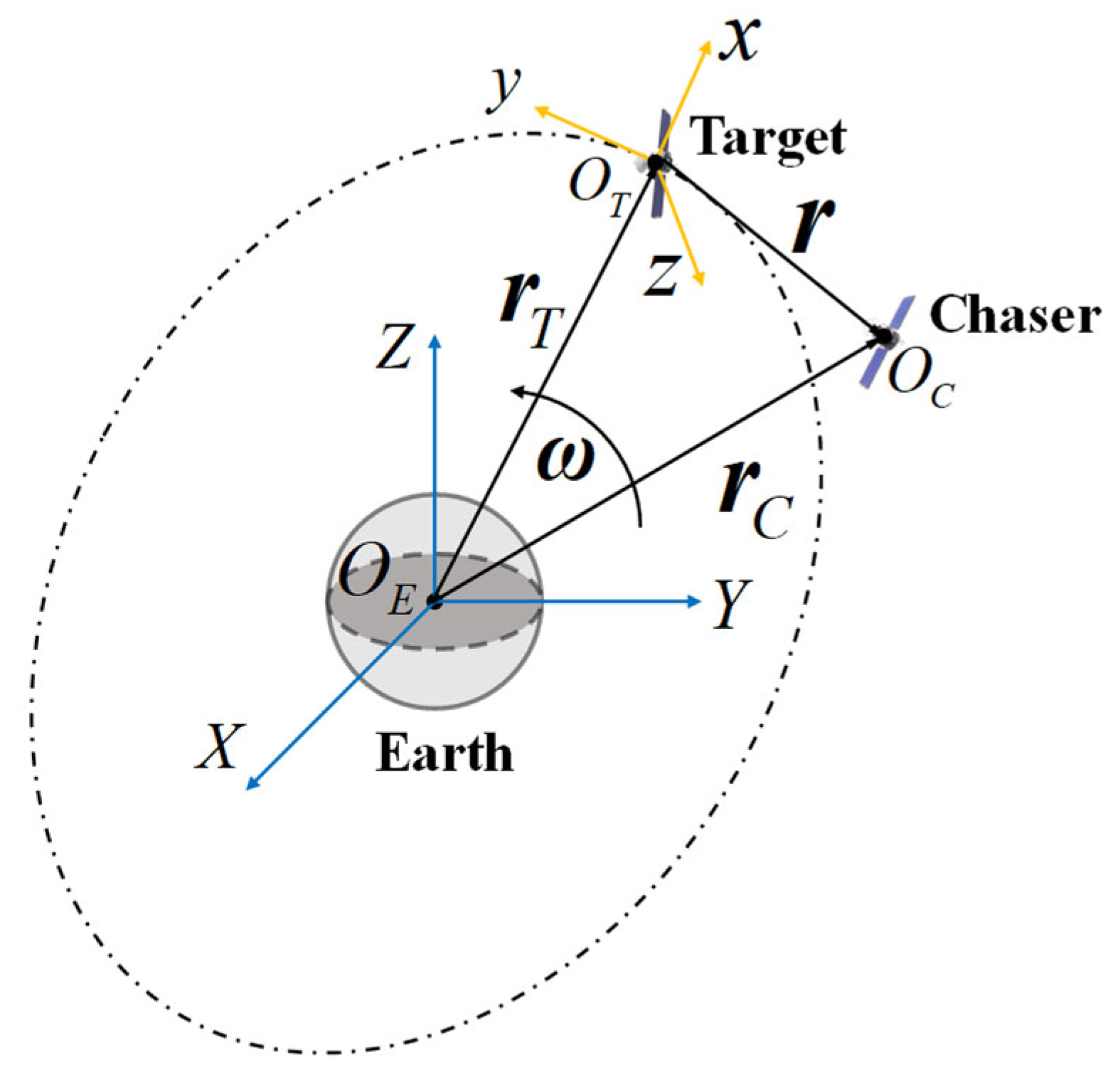
A close-range rendezvous maneuver scenario is discussed in this paper, in which the deputy spacecraft (called the Chaser) passes by the chief spacecraft (called the Target) without colliding. The motion of the Chaser relative to the Target is normally used to illustrate the above proximity. As shown in Figure 1, a local-vertical, local-horizontal (LVLH) coordinate system is defined at the center of the Target and moves with it. The axis, or R-bar, is radially outward. The axis, or V-bar, is perpendicular to the axis and points in the direction of the Target’s motion. The axis, or H-bar, completes the right-hand rule. The position and velocity of the Chaser are indicated by the vectors and , respectively. The superscript represents the transpose operation of a vector or matrix.

Figure 1.
A close-range rendezvous maneuver scenario.
Figure 1 also contains the geocentric equatorial inertial (GEI) coordinate system, which sets its origin at the center of the Earth , the X-axis point in the vernal equinox direction, and the Z-axis point in the direction of the North Pole. The Y-axis is in the equatorial plane and completes the right-hand rule. The vector positions of the Chaser and Target relative to the center of the Earth are denoted by and , accordingly. The angular velocity of the Target is given by the vector , and the scalar indicates its magnitude. Therefore, the vector position of the Chaser satisfies
Differentiating both sides of the Equation (1) twice with respect to time for the GEI coordinate system yields the Chaser’s motion equation as
where the vectors, and , denote the inertial acceleration of the Chaser and the Target. The vector represents the acceleration of the Chaser relative to the Target. The remaining three terms on the right side of Equation (2) are the Coriolis acceleration, the tangential acceleration, and the centripetal acceleration, respectively. The dot notation on signals is defined as the derivative . The double dot [⋅⋅] on signals represents the second-order derivative . The cross-product of the two vectors is indicated by the operator . The following are the operation rules.
where and are the skew-symmetric matrices corresponding to and , respectively.
The following essential assumptions are made to simplify the model of the close-range rendezvous motion. Assume that
- the Target is in a circular orbit near the Earth, and ;
- the orbit radius of the Target . is much larger than the distance between the two spacecraft ;
- both spacecraft are regarded as mass points, and all the orbit perturbations are ignored.
The motion of the Chaser, relative to the Target, can be described by the Clohessy–Wiltshire(CW) equations, based on Equations (2) and (3) and the above assumptions. The CW equations are a set of linear, time-invariant differential equations [47]. The detailed derivation is shown in Chapter 7, reference [48], and the results are given here, directly.
where scalar represents a thrust component of the Chaser’s engine. The mass of the Chaser is given by . Therefore, the relative equations of motion or dynamics equations can be written as a first-order system of variables
or a second-order system of
where
The matrix and denote the -dimensional zero matrix and the identity matrix, respectively.
The analysis of the relative motion of two bodies using the CW equations, which can offer analytical solutions, is widespread and effective [49]. However, the dynamical constraints in the close-range rendezvous process must be balanced against the events, path constraints, and other factors. The analytical solution of the CW equations becomes invalid in this instance. The RPO problem is treated as an optimal control problem (OCP), with various nonlinear and nonconvex constraints in the later subsection.
2.2. Rendezvous Trajectory Optimization
The Chaser completes the objective of approaching the Target with the shortest maneuvering time, or the least fuel consumption, under complicated constraints using the law of relative motion equations. This process is called rendezvous trajectory optimization (RTO). Let be the state variables and be the control variable. Therefore, the OCP version of the RTO in the LVLH coordinate system can be defined as follows:
where scalar signifies the terminal time, which is set as a constant, i.e., the time of RTO is fixed. Scalar is the engine-specific impulse, and is called the sea level gravitational acceleration. The operator here denotes the modulus of a vector. The magnitude of the thrust vector, , must not be greater than the maximum thrust amplitude . The objective function is the integral of thrust to time. The initial condition and the terminal condition for the Chaser are generally determined according to the mission requirements and serve as reference indexes for the accuracy of the subsequent algorithms. The radius of the no-fly zone, denoted by , is the minimum safe distance at which the Chaser will not collide with the Target when approaching it.
The existence of nonlinear or nonconvex terms, such as , and , makes it challenging to obtain the optimal solution to Problem 1. Convexification techniques will be utilized in the following section to convert the original problem into a SOCP problem with a linear objective function and convex constraints.
2.3. Convexification Techniques Applied to RTO
Convexification techniques are used to handle the dynamic constraints and no-fly zone constraints in Problem 1, which was inspired by the study of Aciknese et al. [50,51]. In this study, the key convexification techniques are equivalent transformation, change of variables, and successive approximation, as stated in reference [52].
2.3.1. Equivalent Transformation of the Objective Function
The objective function in Problem 1 cannot become a linear function after discretization, because of the nonlinear factor . Equivalent transformation is used to deal with this situation, as is done in [20]. A slack variable, , is introduced to replace the norm, . The new objective function, , is as follows:
subject to
The transformation from to is equivalent and satisfies the following property at the optimal solution of the problem.
Proof of the equivalence and property is given in Proposition 1, reference [53].
2.3.2. Change of Variables for Dynamic Constraints
The nonlinear terms in dynamic constraints are replaced by linear terms, using a change of variables. The following variables are defined:
The dynamics equations can be rewritten as
where the constant is replaced by for brevity.
Let be the state vector and be the control vector. Therefore, the new description form of the dynamic constraints is as follows:
where
The following is an update to Equation (10)
Then, using the first-order Taylor expansion, the nonlinear term in Equation (19) is approximated at the time, , yielding:
where and the lower bound is .
Now, we can replace Equation (9) with
derived from Equation (15),
From Equation (22), minimizing is equivalent to maximizing , which also implies the optimal fuel consumption. Therefore, replacing with as the objective function is identical.
2.3.3. Linearization of the No-Fly Zone
Setting a no-fly zone is a crucial step in ensuring the safety of the proximity process. The no-fly zone constraint in Problem 1 is defined in the LVLH coordinate system, as shown in Figure 2a. The magnitude of the position vector also represents the distance between the two spacecraft, as the origin is set at the Target centroid. The distance must at least meet the minimum safe distance, , to avoid collisions.
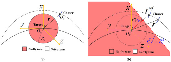
Figure 2.
No-fly zone (red area) and safety zone (white area): (a) Nonconvex no-fly zone; (b) Linear no-fly zone.
The no-fly zone constraint can also be expressed as follows:
The affine function of the position vector is denoted by and approximated using the first-order Taylor expansion at a given reference point . The left side of Equation (23) becomes a linear term.
The trust region constraint is added to guarantee a reasonable approximation of the original value.
where the radius of trust-region ε is positive and small enough. The reference trajectory commonly takes the solution of the last iteration using the SC algorithm, as mentioned in Section 4.4. Inspired by the separating hyperplane theorem [24], we define a separating hyperplane, as shown in Figure 2b, and the describing equation is
where the vector is in the same direction as and the endpoint P is on the boundary of the no-fly zone. The relationship can be denoted as
Based on Equations (24)–(27), we can derive a more intuitive and linear expression of the no-fly zone constraint.
Therefore, the original Problem 1 is converted into a convex Problem 2 through the above convexification techniques.
For Problem 2, the linear time-varying system (LTV) in Equation (29) can be converted from a continuous infinite dimension to a discrete finite dimension by some discretization methods, including the zero-order hold (ZOH), first-order hold (FOH), the Runge–Kutta (RK) method, and the global pseudospectral (PS) method [26]. After discretization, Problem 2 with the convex constraints can obtain the optimal solution by solving a convex programming problem in each iteration until the convergence criterion is satisfied, via the sequential convex (SC) method. In this study, the PS method based on the Birkhoff interpolation is combined with the SC method to solve the RTO problem.
3. Discretization Based on Classical PS Method
3.1. Time-Domain Transformation
In the standard PS method, the time domain is transformed from the physical time t0∈[t0,tf] to the PS time . The mapping function is given as:
where the time mapping factor is defined as .
The discretization method of dynamic constraints, or the transformation of differential equations into algebraic equations, is the focus of this section. For the convenience of explanation, we describe the convex RTO problem as a distilled optimal control problem [35], which simplifies the expression of the boundary constraints and path constraints in Problem 2. For multivariable differential systems, the dynamic constraints follow the vector representation. The time-domain transformation of dynamic constraints is defined as
where the notation ‘′’ denotes the derivative . On the one hand, the boundary constraints were simplified into unified equality constraints
where the dimension of the zero vector was determined by the number of equality constraints. On the other hand, the path constraints included the thrust constraints Equations (18)–(20) and the no-fly zone constraints, Equations (25)–(28), and were simplified into unified inequality constraints.
where the dimension of the zero vector depended on the number of inequality constraints.
As a result, a distilled Problem 3 [39,54] is rephrased in the PS time domain as follows:
3.2. Classical PS Method for RTO
Firstly, an arbitrary grid of distinct nodes is defined in the interval . These nodes are chosen to be the roots of orthogonal polynomials, such as the Legendre polynomials and the Chebyshev polynomials [55]
where the scalar represents the order of the orthogonal polynomials and the number of grid points is . The well-conditioned Gauss–Lobatto (GL) points are chosen as the discrete grid points [35].
Let denote a component of the states on a grid . In the PS theory, the state function can be approximated by the approximation function with the interpolation basis polynomial at these collocation points. For the GL points, the collocation points are the same as the discrete grid points [35]. Therefore, on the grid , we define
where the Lagrange basis functions satisfy the Kronecker delta condition.
The symbol ‘’ can be replaced by the symbol ‘’ when the order tends toward positive infinity.
By introducing Equation (37) into Equation (36), we can get
To simplify the representation, we use instead of , and Equation (38) can be written as .
One of the features of the PS methods, or any Galerkin method, is that the differentiation of the approximation function can be converted into the differentiation of the interpolation polynomial [56,57,58,59]. Consequently, taking the derivative of the time on both sides of Equation (36), we get
Define as the first-order PS differential matrix (PSDM), which is represented as
where is part of . Matrix is also referred to as the differential operator, and it possesses a key characteristic proposed in [14].
where is called the -th order PSDM.
In addition, can also be denoted by the vector .
Equation (39) can be simplified as a matrix-vector product by combining (40) and (42).
Equation (43) is extended to a higher-order form by applying Equation (41) [44]
where denotes the λ-th derivative of with respect to the PS time .
For example, for a second-order system, Equation (44) can be written as
The discretized decision variables are expressed as follows:
where
Therefore, the dynamic constraints in Problem 3 can be discretized as
Defining an overloaded function , Equation (48) can be written as
Based on Equation (43), a new matrix form of differential transformation is given by:
Note that the transpose operation here is because the decision variable is a combination of seven variables, and, after discretization, it is a matrix of , as stated in Equation (46).
Substituting Equation (50) into Equation (49), we get
The dynamic constraints have been turned into a set of algebraic equations, using the differential transformation of the PS method. This means that the RTO problem has become an NLP problem that can be solved by specific solvers [27,28].
For the objective function Equation (21), we make an affine transformation on the time domain, according to Equation (30).
The integral term in the objective function is calculated using the Gauss quadrature formula, as described in [44].
where and
The weight, wi(i = 0,1,2,⋯,N), and the first-order differential matrix, , as mentioned before, have many representations based on different grid values. Readers can refer to [39,44] for further information, owing to the article’s length and major topics.
Due to the length of the paper, the specific derivation process is omitted and the results are directly used in Section 4.4. Readers can refer to Sagliano’s research [58] for a detailed processing framework. Thus, the PS transformation of the boundary constraints and the path constraints on the grid remains as in Problem 3. As a result, Problem 3 on the discretized points can be rewritten, using the first-order differential PS method (FDPSM).
4. Well-Conditioned Birkhoff PS Methods for Multiple Dynamic Systems
4.1. Basic Properties of Birkhoff Interpolation
As the basis of the Birkhoff PS method, the Birkhoff interpolation is regarded as a new extension of the Lagrange interpolation and Hermite interpolation [60,61]. Unlike the Lagrange interpolation in Equation (36), the Birkhoff interpolation function is a mix of various orders of the derivatives of a function [60]. Two general forms of the Birkhoff interpolation, based on the first-order or second-order boundary value problems (BVPs), were proposed in [44]. The dynamics system in the RTO can be a first-order system about , as indicated in Equation (5), or a second-order system about , as shown in Equation (6).
Let be a first-order, continuously bounded function on the grid points . Therefore, a first-order Birkhoff interpolation polynomial is defined as [39],
where the Birkhoff interpolation basis polynomials, , can be regarded as the counterpart of the Lagrange polynomials [39] and must satisfy
The interpolation polynomial needs to meet the interpolation conditions, which can be regarded as an extension of Equation (38)
Let , thus a first-order Birkhoff PS integral matrix (FBPSIM) is defined as
and satisfies that
where the matrix is generated by substituting the initial row of with . The calculation of and the property of and in Equation (60) are omitted here, and the detailed derivation can be found in Section 4.1, reference [44]. Therefore, the Equation (56) can be rewritten in vector-matrix form:
where
Let be a second-order, continuously bounded function on the grid points . Similarly, a second-order Birkhoff interpolation polynomial can be written as
the interpolation conditions Equations (57) and (63) can be rewritten as
and
Let , thus a second-order Birkhoff PS integral matrix (SBPSIM) is defined as
and satisfies that
where the matrix can be produced by replacing the initial and last rows of the matrix with and , respectively. The detailed derivation can be found in Sections 3.1 and 3.2, reference [44]. The vector-matrix form of Equation (63) is given as
where
4.2. The First-Order Birkhoff PS Method for RTO
The first-order Birkhoff PS method (FBPSM) is based on the first-order Birkhoff interpolation in Equation (56). For the first-order system, we approximate the state function by applying Equation (56) to Problem 3. The approximation function on the grid can be rewritten as
where the vector is regarded as the unknown optimization variable and satisfies Equation (57). Taking the derivative of the time on both sides of Equation (70), we get
As in Equation (61), the vector-matrix form of Equation (70) is given by
Therefore, the vector-matrix form of Equation (71) can be given by
where represents the derivative of over .
According to Equations (43) and (70), it can be deduced that
where
Applying the property of the FBPSM to Problem 3, the discretized unknown variables can be denoted by
Combining the decision variables defined in Equation (46), the dynamic constraint in Equation (51) is rewritten as
where
Therefore, Problem 3 on the discretized points is given by using the first-order Birkhoff PS method (FBPSM).
.
4.3. The Second-Order Birkhoff PS Method for RTO
The second-order Birkhoff PS method (SBPSM) is based on the second-order Birkhoff interpolation in Equation (63). The Equations (13) and (14) in the dynamic constraint can be expressed in a second-order form.
Let set be a component of . Applying Equation (63) to Equation (81) on the grid , we get
where the vector is the unknown optimization variable, is the approximation function, and satisfies the condition in Equation (64). Differentiating twice on both sides of Equation (82), we get
The vector-matrix form of Equation (82) can be written as
where and is the SBPSIM defined in Equation (66).
The vector-matrix form of Equation (83) is given as
where represents the derivative of over .
Combining the properties of Equations (45) and (67), we have
where
Applying the SBPSM to Problem 3, the unknown optimization variables are defined as
The new discretized representation of the decision variables is given as
Thus, Equation (81) is rewritten as
where
In addition, the FBPSM is used to deal with the remaining first-order equation, Equation (15). We define the unknown variable as
The new discretized representation of the decision variables is given as
Thus, Equation (15) can be rewritten as
where
Therefore, Problem 3 on the discretized points is given by using the second-order Birkhoff PS method (SBPSM).
4.4. Sequential Convex Algorithm for RTO
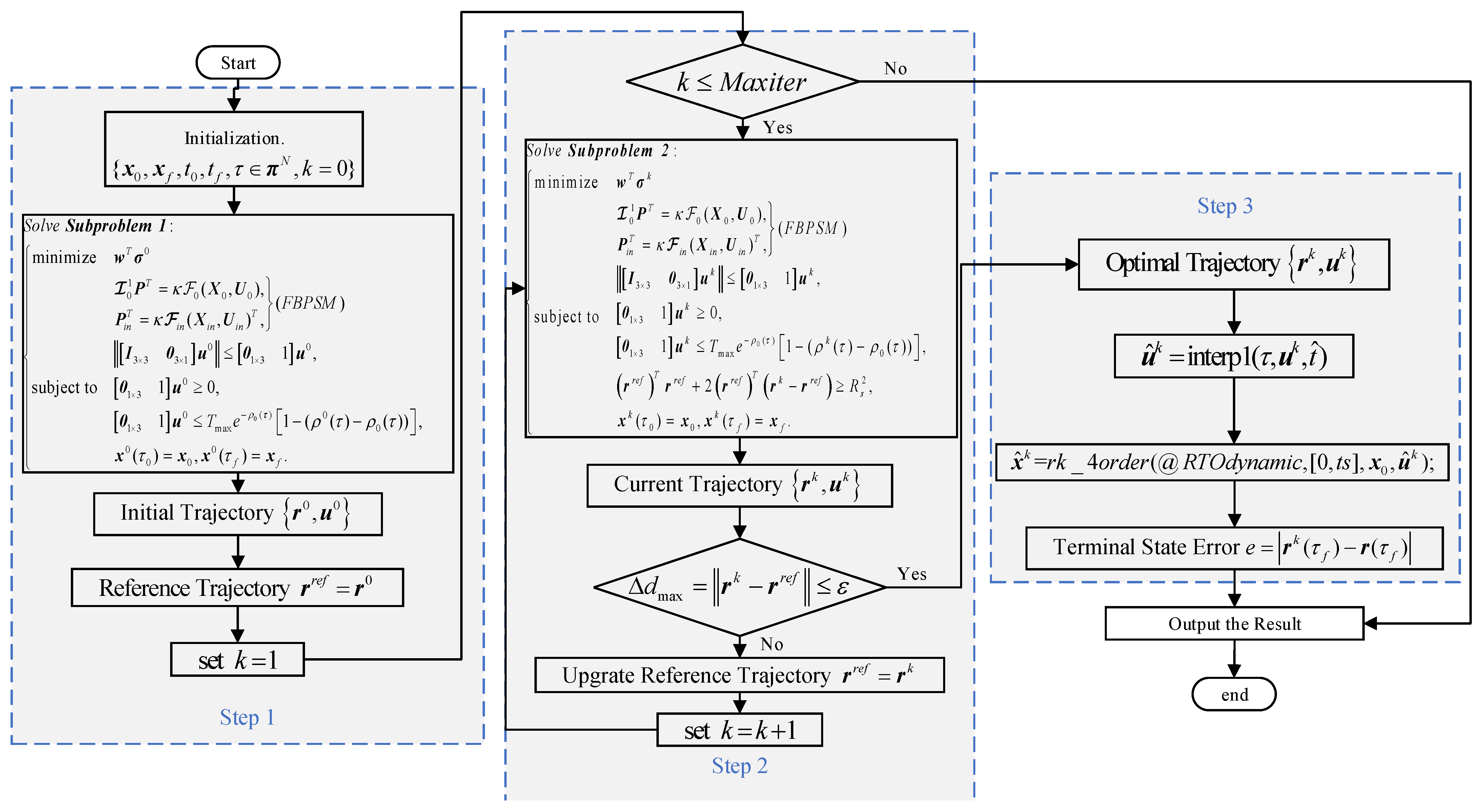
In this section, the sequential convex (SC) algorithm is used to solve the finite convex problem after the convexification and discretization. The main idea is to solve a series of convex subproblems to converge to the optimal solution . The iteration process via the SC algorithm is described in Algorithm 1.
| Algorithm 1 The iteration process of the SC algorithm |
| SC Algorithm for RTO |
Input: The initial state x0 = [r0,v0] and the terminal state xf = [rf,vf]; the initial mass of the Chaser m0; the initial and terminal time [t0,tf] .
|
Step 1: Calculate the initial trajectory r0 without the no-fly constraint and set it as the reference trajectory rref of the first iteration. Go to step 2. |
Step 2: Start the loop until meeting the trust-region constraint. |
1. For k = 1:Maxiter; |
2. Calculate the current trajectory {rk,uk}; |
3. Calculate the maximum distance Δdmax between rk and rref; |
4. Check the trust-region constraint: |
If Δdmax ≤ ε established, exit the loop and go to step 3; otherwise, set rref = rk and continue.
|
5. End. |
Step 3: Evaluate the accuracy of the solution e. Go to step 4. |
Step 4: Output the result. The optimal trajectory and optimal control are {r*,u*} ; the optimal objective value is j*. |
Remark 1.
The convergence of the SC algorithm is significantly influenced by a good initial trajectory. We propose to cancel the no-fly zone constraint to achieve this goal, which is also given by the subsequent simulation. Therefore, the first subproblem is given as
Remark 2.
In step 2, the subproblem required to be solved in the-th iteration with all constraints is as follows:
The parameter maxiter in step 2 represents the SC algorithm’s maximum number of iterations. The SC algorithm does not converge to the optimal solution, fulfilling the trust-region condition, if takes the value of maxiter. It’s feasible to replace more relaxed convergence conditions or add the mesh points to improve the convergence of the SC algorithm.
Remark 3.
In step 3, we linearly interpolate the optimal controlof the iterative result of the SC algorithm, integrate the original dynamic equation with fourth-order Runge–Kutta to obtain the terminal state, and then compare the terminal valueto the given accurate valueto calculate the terminal error, which is used as the algorithm’s accuracy index.
The stepsize of the fourth-order Runge–Kutta integral was 0.001 in the PS time domain.
Remark 4.
To simplify the problem, only one no-fly zone constraint is considered in step 2, and the geometric shape is a sphere or an ellipsoid. Readers can learn more about the excellent work on multiple no-fly zones and complex geometries through [62,63].
For the ease of comprehension, we provide the complete process framework of the SC algorithm, using the FBPSM discretization method as an illustration, in Figure 3.
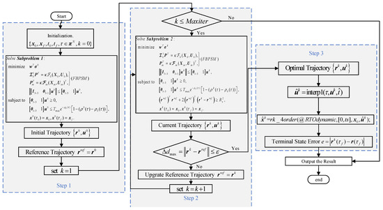
Figure 3.
The complete process framework of the SC algorithm takes the FBPSM discretization method as an example.
5. Numerical Simulation
In this section, two cases are given to illustrate the feasibility and advantages of the proposed SC algorithm, based on the first-order and second-order Birkhoff pseudospectral discretization methods (FBPSM and SBPSM). As comparison methods, other discretization techniques, such as the zero-order hold (ZOH) [26] and the classic pseudospectral method, as mentioned in Section 3 (FDPSM), are chosen.
All numerical simulations were performed on a desktop with an Intel (R) Core (TM) i5-10400 (CPU 2.90 GHz) and with MATLAB version 2020a. The modeling tool is Yalmip [64] and the solver tool is Mosek [21]. Additionally, we found through research that the preprocessing option of the MOSEK solver significantly affects the results of the solution. Therefore, we changed the value of the option “MSK_IPAR_PRESOLVE_USE” to OFF and the reason is given in the following section.
Nondimensionalization is an effective method to simplify the calculation and improve accuracy. Table A1 in Appendix A provides a list of the principal dimensionless units. The radius of the earth, , is 6378.14 km, and the gravitational acceleration, , is 9.807 m/s. The value of the geocentric gravitational constant, , is . The satellite completes the maneuvering and rendezvous at an orbital altitude, , of 600 km. The initial mass of the Chaser, , is 1000 kg. The initial parameters of the simulations are dimensionless, as shown in Table A2, Appendix A. Note that the variables contained in this section tables and figures are defined in the LVLH coordinate system.
5.1. Case 1: Excellent Computational Efficiency and Solution Accuracy under Different Grid Points
We set up several numerical tests with different grid points to evaluate the accuracy of the solution and the computational efficiency of the proposed methods. In general, the grid points of the ZOH method are evenly distributed. The Runge phenomenon [54] becomes increasingly prevalent as the number of grid points rises, which reduces the precision of the solution. Although the FDPSM improves the situation to a certain extent, it destroys the sparsity of the system, which is manifested in the exponential growth of the condition number of the coefficient matrix and leads to a longer solution time. This situation can be improved by using the proposed methods, based on the Birkhoff interpolation. Given that reference [39] contains the outcomes of the first-order system, we just provide the change law of the condition number of the coefficient matrix under the second-order system, as depicted in Figure A1, Appendix A. The definitions of three types of coefficient matrices can be found in Section 5 of [39]. The condition number, based on the second-order Birkhoff PSIM , shows an obvious decrease from to , even with an invariable constant , which indicates that the Birkhoff PS method also has a significant effect on improving the condition number of the second-order system.
First, we divided the tests into seven groups, each with a number of grid points ranging from 30 to 210. The total time, , required to arrive at the optimal solution is utilized as the evaluation criterion for computational efficiency, and it primarily involves the two stages of problem-modeling and solver-solving. The expression is as follows:
where the term represents the time of solving Subproblem 1 in Equation (95), the intermediate-term denotes the time of solving Subproblem 2 in Equation (96), and is the number of iterations. The term is the time of the remaining parts in Figure 3 and is equal, in principle, for the above four methods. The terminal state error, , which is stated in Equation (97) of remark 3, is used to determine the accuracy of the solution. The value of the performance index, , is related to the optimality of the solution. The statistical results are shown in Table 1.

Table 1.
The statistical results under different grid points N.
The results in Table 1 demonstrate that the number of grid points, , does have an impact on the computational efficiency and some new findings are given here. The indicators of the final three methods show a minimal difference, whereas the ZOH method’s total time, , has nearly tripled and has a significant terminal error, according to the findings of the first four groups. However, when is selected as 150 or more, the total solution time of the FDPSM rises sharply, which is roughly three times that of the Birkhoff PS methods.
According to our analysis, the Birkhoff PS methods decrease the condition number of the coefficient matrix, enhance the dynamics equations, and thus shorten the modeling time of the optimization problems. Additionally, we discover that the total solution time of the SBPSM is less than the FBPSM. In comparison to the FDPSM and FBPSM, the SBPSM reduces the number of unknown variables, which, in turn, reduces the dimension of the problem and ultimately speeds up the solving process. Figure 4 illustrates the model time and solver time at various grid points and supports the validity of the conclusion. For example, the model time of the FDPSM in Figure 4a is greater than that of the FBPSM and SBPSM, when is set as 150 or more. In contrast, the two first-order approaches take longer to solve the problem than the SBPSM in Figure 4b.
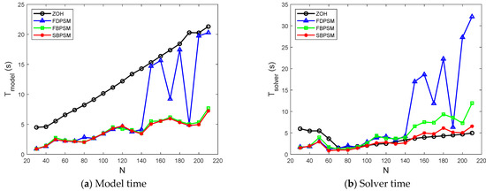
Figure 4.
The curve of model time and solver time under the different number of grid points.
A perfect discretization method has a modest terminal state error, in addition to a brief total solution time. Figure 5 demonstrates that, although the terminal error of ZOH steadily lowers as the number of grid points increases, it is still higher than that of other discretization approaches. In terms of the solution accuracy, this result demonstrates that the ZOH is inferior to the pseudospectral discretization method. The outcomes also indicate that the new discrete approach, which is based on the Birkhoff interpolation, inherits the superior qualities of the conventional pseudospectral method. Figure 6 displays the position errors as measured by the difference between the optimal trajectory and the propagated trajectory in both the x-axis and y-axis directions. The solution accuracy of the SBPSM is higher because, during the entire maneuver, the error of the SBPSM is smaller than the result of the ZOH in both directions.
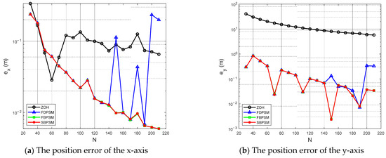
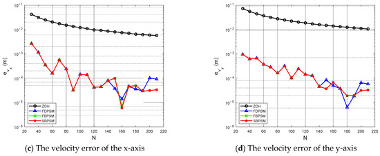
Figure 5.
The terminal position and velocity error under the different number of grid points.
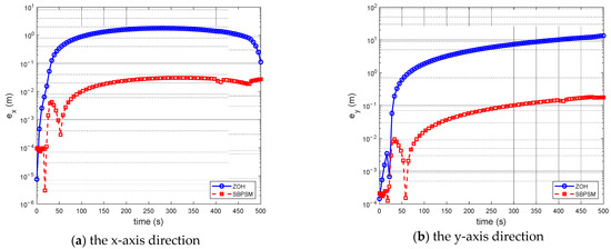
Figure 6.
The position errors, as measured by the difference between the optimal trajectory and the propagated trajectory. (N = 90).
Furthermore, we investigated the impact of the grid points count on the no-fly zone and thrust constraints. The findings indicate that increasing the grid points was necessary to improving the practicality of the ideal solution and the maneuverability. Readers can refer to Appendix B for details.
In summary, to ensure that the constrained problem has an optimal solution, we need to set the number of grid points, , to be large enough, which will reduce the computational efficiency and solution accuracy. The proposed methods based on the first-order and second-order Birkhoff interpolation can significantly improve the efficiency of the solution, while maintaining high accuracy.
5.2. Case 2: Sensitivity Analysis under Different Conditions
In this section, the performance of the proposed algorithm was verified by a sensitivity analysis under different test conditions. The main measurement indicators were the total solution time, the number of iterations, and the terminal state error. Firstly, two conditions were considered: the type of grid points, and the shape of the no-fly zone. By adding the perturbation to the initial position in the y-axis direction, a Monte Carlo analysis was conducted. The grid points were chosen between LGL and CGL [26] for the fuel optimization problem over a fixed time interval. In addition to the sphere, the ellipsoid was also selected for the shape of the no-fly zone. Table A2 in Appendix A displays the shape characteristics of no-fly zones. The value of the perturbation was randomly generated within the range of [−1,1] m and the number of simulation groups was set as 300. The different simulation settings are denoted by the titles of the subgraphs in Figure 7 and Figure 8, and three pseudospectral methods are described in the legend. The ZOH technique is not considered in this section, due to the uniform distribution of the grid points and the difficulty in meeting the accuracy requirements with the maximum number of iterations, due to the huge terminal position error.

Figure 7.
The curves of the total solution time Ttotal under different types of grid points and no-fly zones.

Figure 8.
The curves of the number of iterations Siter under different types of grid points and no-fly zones.
It is clear from Figure 7 that the FBPSM and SBPSM have more stable total solution times than the FDPSM, as evidenced by the roughly linear growth and square growth trends once the grid point exceeds 100, respectively. At the same time, the SBPSM performs marginally better than the FBPSM, which is in line with the analysis in the preceding section. The number of iterations of the three methods in Figure 8 displays a “steady” fluctuation, but the interpretation is different. The fact that the number of iterations fluctuates between five and eight for the FBPSM and SBPSM indicates that the two approaches can steadily converge to the optimal solution. The approach of the FDPSM cannot ensure a stable convergence to the optimal solution since the number of iterations varies between the maximum and the finite number of iterations (). The findings demonstrate that the SC algorithm, based on the FBPSM and SBPSM, is suitable for the four circumstances listed and can maintain a faster solution and more stable convergence when there are more grid points.
The purpose of the Monte Carlo simulation tests is to evaluate the sensitivity of these three methods in dealing with the initial state perturbations. The tests are divided into two scenarios: and . Each test only changes the initial position in the -axis direction, and the perturbations are randomly generated. The total solution time, , and the terminal position error, , are chosen as the evaluation indices. The results are presented in Appendix A.
A visual evaluation model is created in Figure A2 by using the total solution time as the vertical axis and the terminal position error as the horizontal axis. The overall performance of this method is better the closer the results are to the lower left corner. In scenario 1, as depicted in Figure A2a, the output from the three algorithms reveals two identical clustering zones, with an error line of 0.4 m serving as the dividing line. The increase in the terminal position accuracy is accompanied by a jump in the total solution time, which rises from the right side of the dividing line to the left side of the dividing line, with an increase of roughly two seconds. The clustering regions’ findings indicate that, while the solution accuracy may increase in some ranges, the total solution time may remain unchanged. Figure A2b depicts the differential distribution between the FDPSM and the Birkhoff pseudospectral methods results in scenario 2. Although the majority of the FDPSM results are clustered around , there are some scattered points in a wider range in both the horizontal and vertical directions. The results of the FBPSM and the SBPSM are more concentrated, and the advantage in the total solution time can be perceived. To some extent, the approach of the FDPSM is more sensitive to the initial position disturbance.
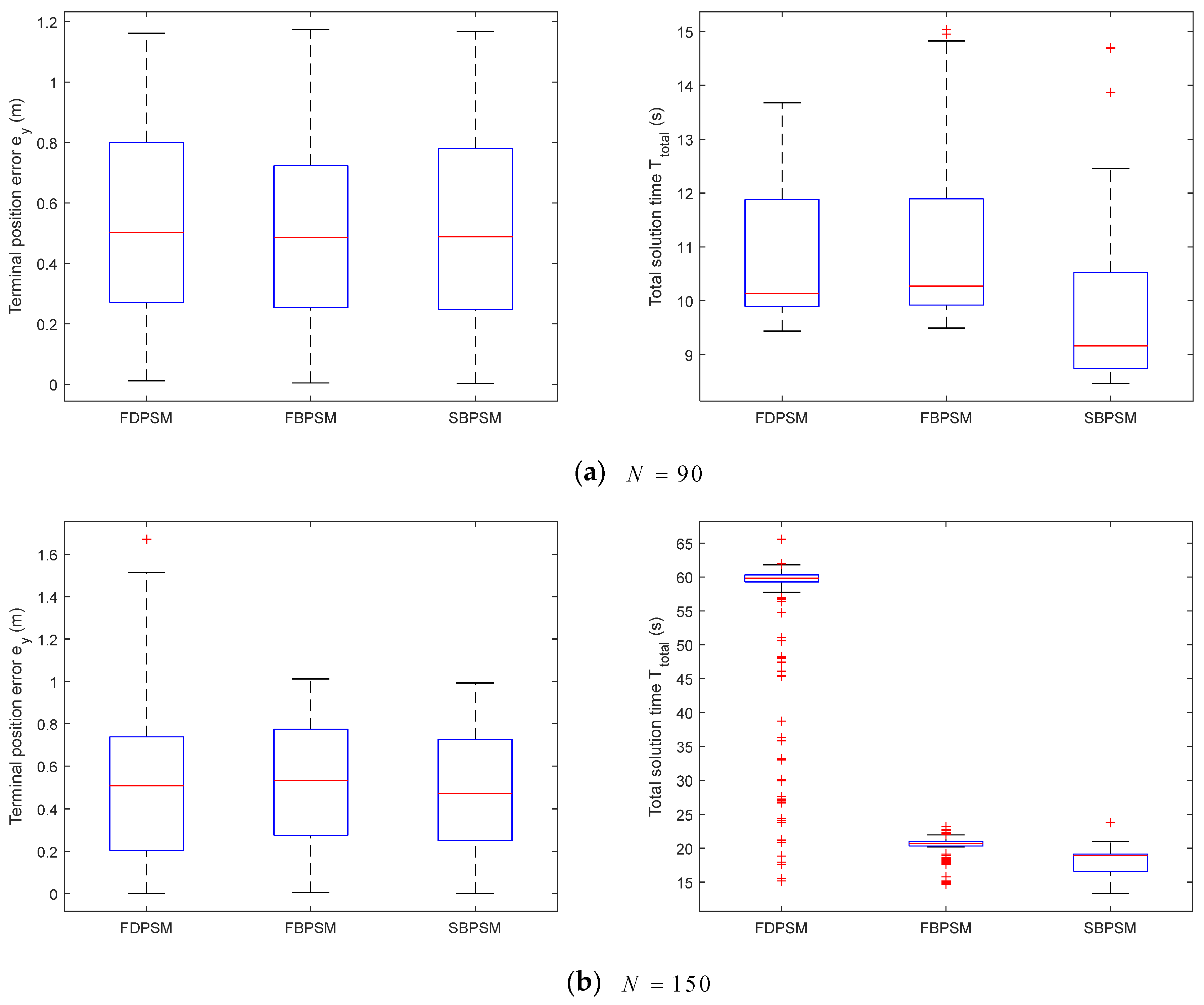
Figure A3 illustrates the findings of our quantitative analysis of the Monte Carlo simulation data, which is an addition to the results of the qualitative study discussed above. The terminal position errors of the three methods are primarily spread in the range of [0,1.2] m depicted in Figure A3a, with a median value of roughly 0.5 m. The highest limit of the FBPSM is closer to 15 s in terms of total solution time, whereas the majority of the SBPSM outcomes (about 75%) are 1.5 s faster than the other two approaches. When the number of grid points is set to 150, in Figure A3b, the terminal position error of the FDPSM spreads to 1.5 m, the median value of the total solution time rises from 10 s to 60 s, and the properties of the centralized distribution deteriorate. The original error level is maintained by the FBPSM and SBPSM, and the median value of the total solution time is 21 s and 19 s, respectively. In terms of both the solution accuracy and computational efficiency, the Birkhoff pseudospectral approaches are more stable than the FDPSM.
Through sensitivity analysis, it is found that, compared with the FDPSM, the Birkhoff pseudospectral methods have the following advantages: (i) they can converge to the optimal solution steadily at a faster speed and are suited for two different types of grid points and no-fly zones. (ii) In the case of the initial position disturbance, they can maintain a more stable terminal position error distribution and higher computational efficiency. (iii) Under the same conditions, the second-order Birkhoff pseudospectral method (SBPSM) is better than the first-order Birkhoff pseudospectral method (FBPSM), both in solution time and the robustness against the initial position disturbances.
6. Conclusions
With the increase in the series of space missions, such as the space station construction, on-orbit maintenance, material supply, and astronaut rotation, in the future, the RPOs will play a more important role. The popularization of automatic rendezvous technology will be of great significance to save human and material resources. The method proposed in this paper combines convex optimization technology with the Birkhoff pseudospectral method. The advantages of convex optimization techniques, such as polynomial complexity and global optimal solution, are inherited. At the same time, the pseudospectral method, based on the Birkhoff interpolation, overcomes the shortcomings of the original, traditional differential operator pseudospectral method. With the increase of the polynomial order, , the proposed methods can not only maintain the solution accuracy but also greatly improve the computational efficiency. Especially for the dynamic system, the second-order Birkhoff pseudospectral method will have a more obvious improvement effect. Under certain conditions, the improvement of the computational efficiency can be expanded by up to three times. This work discovery will provide a possible basis for realizing spacecraft autonomous online real-time trajectory planning. Further exploring the computational performance of the proposed method and striving for practical onboard applications will be the goal of our future work.
Author Contributions
Conceptualization, Z.Z., D.Z. and X.L.; methodology, Z.Z. and D.Z.; software, Z.Z.; validation, Z.Z., D.Z. and X.L.; formal analysis, Z.Z.; investigation, Z.Z.; resources, Z.Z.; data curation, D.Z. and X.L.; writing—original draft preparation, Z.Z.; writing—review and editing, D.Z. and X.L.; visualization, C.K. and M.S.; supervision, D.Z.; project administration, D.Z.; funding acquisition, D.Z. All authors have read and agreed to the published version of the manuscript.
Funding
This research was funded by the National Key Research and Development Program of China, grant number 2021YFC3090401.
Informed Consent Statement
Not applicable.
Data Availability Statement
Not applicable.
Acknowledgments
We thank the anonymous reviewers for providing many detailed comments. Their comments greatly improved the quality of this paper.
Conflicts of Interest
The authors declare no conflict of interest.
Appendix A
Appendix A contains some of the tables and result charts that are needed for Chapter 5.
Table A1.
Dimensionless units and values for Section 5.1.
Table A1.
Dimensionless units and values for Section 5.1.
| Dimensionless Unit | Value |
|---|---|
| Length | |
| Speed | |
| Time | |
| Acceleration | |
| Mass | |
| Force |
Table A2.
Initialization parameters of the RTO problem for Section 5.1.
Table A2.
Initialization parameters of the RTO problem for Section 5.1.
| Initialization Parameters | Value |
|---|---|
| Initial Mass | |
| Initial and Terminal Time | |
| Initial and Terminal Position | |
| Initial and Terminal Speed | |
| No-fly Zone Radius | |
| Maximum Thrust Limit | |
| Reciprocal of effective exhaust velocity |
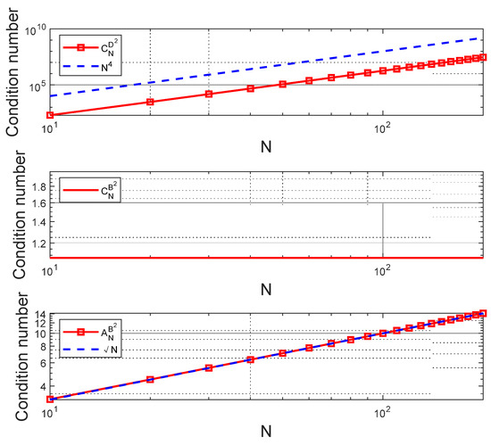
Figure A1.
The change law of condition number of the coefficient matrix under the second-order system.
Figure A1.
The change law of condition number of the coefficient matrix under the second-order system.
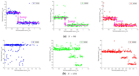
Figure A2.
6 × 300 groups of Monte Carlo simulation results based on initial position perturbation .
Figure A2.
6 × 300 groups of Monte Carlo simulation results based on initial position perturbation .


Figure A3.
Distribution statistics data of 6 × 300 groups of Monte Carlo simulation results.
Figure A3.
Distribution statistics data of 6 × 300 groups of Monte Carlo simulation results.
Appendix B
Figure A4a illustrates that the no-fly zone constraint fails when N is 30 because the Chaser’s optimal trajectory, as determined by the FDPSM, passes across the no-fly zone. The optimal trajectory, as seen in Figure A4b, flies around the boundary of the no-fly zone and finally reaches the desired position safely when there are 120 grid points. This demonstrates that the effectiveness of the no-fly zone constraint is correlated with the number of grid points.
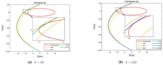
Figure A4.
The two-dimensional trajectory of the Chaser satellite approaches the spherical no-fly zone.
Figure A4.
The two-dimensional trajectory of the Chaser satellite approaches the spherical no-fly zone.
Generally, the distribution characteristics of the Chebyshev–Gauss–Lobatto (CGL) grid points cluster at both ends and are sparse in the middle. As a result, when N is too small, there are few interpolation points near the no-fly zone, causing the trajectory to directly cross this area, as illustrated in Figure A5. Finally, the optimal trajectory fails to meet the no-fly zone constraint, and the two satellites may collide in the close-range rendezvous mission. There are enough interpolation nodes close to the no-fly zone’s boundary when is a suitable value. Through the successive iterative optimization process, the Chaser satellite avoids the no-fly zone along the optimal trajectory and reaches the endpoint, as shown in Figure A6. The results and conclusions obtained by using the FBPSM and SBPSM are consistent with the above findings using the FDPSM. Therefore, after assessing the computational efficiency and precision of the solution, the Birkhoff pseudospectral method is unquestionably a better option when the number of grid points must be raised to satisfy the requirements.
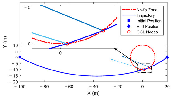
Figure A5.
Distribution of trajectory grid points (red circles) near the no-fly zone. (N = 30).
Figure A5.
Distribution of trajectory grid points (red circles) near the no-fly zone. (N = 30).
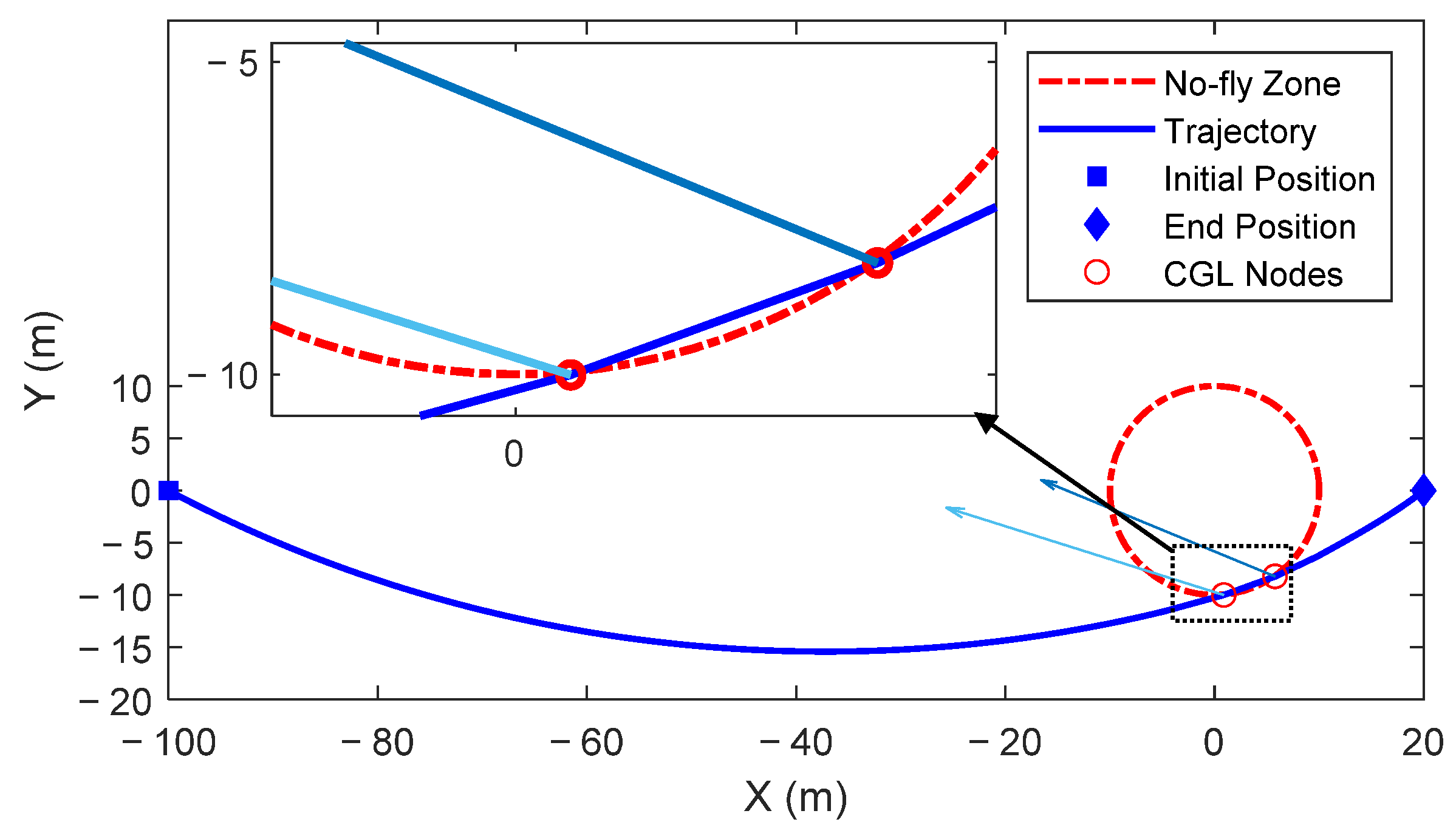
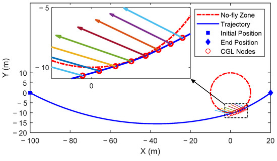
Figure A6.
Distribution of trajectory grid points near the no-fly zone. (N = 120).
Figure A6.
Distribution of trajectory grid points near the no-fly zone. (N = 120).
Figure A7 depicts the variation curve of the component and the magnitude of the Chaser’s thrust when the number, , is taken as 30 and 120, respectively. First, from the two subgraphs on the right, it can be found that the slack variable, , is completely consistent with the change curve of the thrust magnitude, . This illustrates that the lossless convexity operation is effective and verifies that the solution of the relaxed Problem 2 is equivalent to the original Problem 1. From the subgraphs of the thrust component, it can be found that the thrust mainly acts on the -axis and the -axis, which is also in line with the characteristics of the maneuvering transfer in the plane, with minimum fuel consumption. Moreover, when the number of grid points is small, the change in thrust is relatively stable and slow, especially when passing through the no-fly zone, when the working time of the whole engine is about 80 s. In sharp contrast, when is 120, the satellite makes a rapid maneuver response when approaching the no-fly zone, which lasts only 15 s. From the previous result analysis, it is known that, in the end, the former mission failed, while the latter perfectly avoided the no-fly zone and reached the destination.
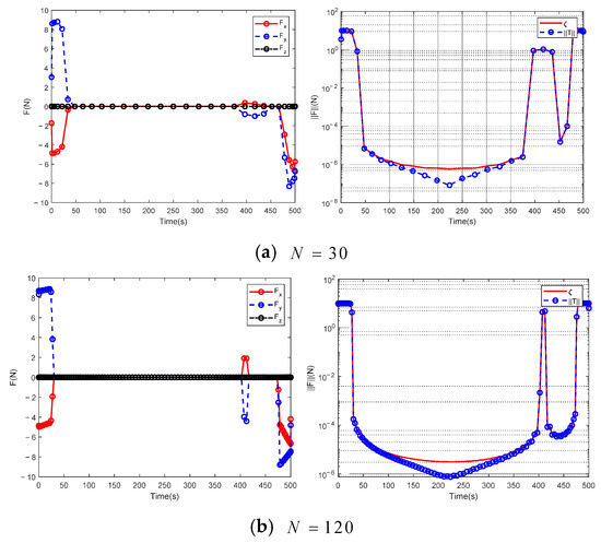
Figure A7.
The curve of the thrust components and magnitude for the spherical no-fly zone when N is 30 and 120,respectively.
Figure A7.
The curve of the thrust components and magnitude for the spherical no-fly zone when N is 30 and 120,respectively.
References
- Fehse, W. Automated Rendezvous and Docking of Spacecraft; Cambridge University Press: Cambridge, UK, 2003. [Google Scholar] [CrossRef]
- Chamberlin, J.A.; Rose, J.T. Gemini rendezvous program. J. Spacecr. Rocket. 1964, 1, 13–18. [Google Scholar] [CrossRef]
- Young, K.A.; Alexander, J.D. Apollo lunar rendezvous. J. Spacecr. Rocket. 1970, 7, 1083–1086. [Google Scholar] [CrossRef]
- Murtazin, R.F.; Budylov, S.G. Short rendezvous missions for advanced Russian human spacecraft. Acta Astronaut. 2010, 67, 900–909. [Google Scholar] [CrossRef]
- Goodman, J.L. History of space shuttle rendezvous and proximity operations. J. Spacecr. Rocket. 2006, 43, 944–959. [Google Scholar] [CrossRef]
- Woffinden, D.C.; Geller, D.K. Navigating the road to autonomous orbital rendezvous. J. Spacecr. Rocket. 2007, 44, 898–909. [Google Scholar] [CrossRef]
- Luo, Y.; Zhang, J.; Tang, G. Survey of orbital dynamics and control of space rendezvous. Chin. J. Aeronaut. 2014, 27, 1–11. [Google Scholar] [CrossRef]
- Morante, D.; Sanjurjo Rivo, M.; Soler, M. A Survey on Low-Thrust Trajectory Optimization Approaches. Aerospace 2021, 8, 88. [Google Scholar] [CrossRef]
- Bucchioni, G.; Innocenti, M. Rendezvous in Cis-Lunar Space near Rectilinear Halo Orbit: Dynamics and Control Issues. Aerospace 2021, 8, 68. [Google Scholar] [CrossRef]
- Kawano, I.; Mokuno, M.; Kasai, T.; Suzuki, T. Result and evaluation of autonomous rendezvous docking experiment of ETS-VII. Guid. Navig. Control Conf. Exhib. 1999, 38, 105–111. [Google Scholar] [CrossRef]
- Thomas, M.D.; David, M. XSS-10 microsatellite flight demonstration program results. In Spacecraft Platforms and Infrastructure; SPIE: Orlando, FL, USA, 2004; Volume 5419, pp. 16–25. [Google Scholar]
- Timothy, E.R. Demonstration of autonomous rendezvous technology (DART) project summary. In Space Systems Technology and Operations; SPIE: Orlando, FL, USA, 2003; Volume 5088, pp. 10–19. [Google Scholar]
- Manny, R.L.; Chih-Tsai, C.; Michael, W.B.; Thomas, P.W.; David, L.C.; William, B.G.; Peter, W.S.; Peter, A.S.; Mark, A.L. Orbital express autonomous rendezvous and capture sensor system (ARCSS) flight test results. In Sensors and Systems for Space Applications II; SPIE: Orlando, FL, USA, 2008. [Google Scholar]
- Zhou, J. Tiangong-1/Shenzhou-8 rendezvous and docking process. In Space Rendezvous and Docking Technology; National Defense Industry Press: Beijing, China, 2013; pp. 56–62. [Google Scholar]
- Yang Cheng, Z.X. Tianzhou-3 Completes Autonomous Rapid Rendezvous and Docking. Available online: https://www.chinadefenseobservation.com/?p=8682 (accessed on 20 September 2021).
- Trent, J.; Perrotto, J.B. Spacex Dragon Attached to Space Station in Spaceflight First. Available online: https://www.nasa.gov/home/hqnews/2012/may/HQ_12-172_SpaceX_Dragon_Berth.html (accessed on 25 May 2012).
- Betts, J.T. Survey of numerical methods for trajectory optimization. J. Guid. Control Dyn. 1998, 21, 193–207. [Google Scholar] [CrossRef]
- Rao, A.V. A survey of numerical methods for optimal control. Adv. Astronaut. Sci. 2010, 135, 1–32. [Google Scholar]
- Trélat, E. Optimal control and applications to aerospace: Some results and challenges. J. Optim. Theory Appl. 2012, 154, 713–758. [Google Scholar] [CrossRef]
- Tang, G.; Jiang, F.; Li, J. Fuel-Optimal Low-Thrust Trajectory Optimization Using Indirect Method and Successive Convex Programming. IEEE Trans. Aerosp. Electron. Syst. 2018, 54, 2053–2066. [Google Scholar] [CrossRef]
- Andersen, E.D.; Roos, C.; Terlaky, T. On implementing a primal-dual interior-point method for conic quadratic optimization. Math. Program. 2003, 95, 249–277. [Google Scholar] [CrossRef]
- Guo, X.; Zhu, M. Direct trajectory optimization based on a mapped Chebyshev pseudospectral method. Chin. J. Aeronaut 2013, 26, 401–412. [Google Scholar] [CrossRef]
- Benson, D.A.; Huntington, G.T.; Thorvaldsen, T.P.; Rao, A.V. Direct Trajectory Optimization and Costate Estimation via an Orthogonal Collocation Method. J. Guid. Control Dyn. 2006, 29, 1435–1440. [Google Scholar] [CrossRef]
- Boyd, S.; Boyd, S.P.; Vandenberghe, L. Convex Optimization; Cambridge University Press: Cambridge, UK, 2004. [Google Scholar]
- Oumer, A.M.; Kim, D.-K. Real-Time Fuel Optimization and Guidance for Spacecraft Rendezvous and Docking. Aerospace 2022, 9, 276. [Google Scholar] [CrossRef]
- Malyuta, D.; Reynolds, T.; Szmuk, M.; Mesbahi, M.; Acikmese, B.; Carson, J.M. Discretization Performance and Accuracy Analysis for the Rocket Powered Descent Guidance Problem. In Proceedings of the AIAA Scitech 2019 Forum, San Diego, CA, USA, 7–11 January 2019. [Google Scholar] [CrossRef]
- Wächter, A.; Biegler, L.T. On the implementation of an interior-point filter line-search algorithm for large-scale nonlinear programming. Math. Program. 2006, 106, 25–57. [Google Scholar] [CrossRef]
- Gill, P.E.; Murray, W.; Saunders, M.A. SNOPT: An SQP Algorithm for Large-Scale Constrained Optimization. SIAM Rev. 2005, 47, 99–131. [Google Scholar] [CrossRef]
- Betts, J.T. Practical Methods for Optimal Control and Estimation Using Nonlinear Programming; Cambridge University Press: Cambridge, UK, 2009. [Google Scholar]
- Betts, J.T.; Huffman, W.P. Mesh refinement in direct transcription methods for optimal control. Optim. Control Appl. Methods 1998, 19, 1–21. [Google Scholar] [CrossRef]
- Elnagar, G.; Kazemi, M.A.; Razzaghi, M. The pseudospectral Legendre method for discretizing optimal control problems. IEEE Trans. Autom. Control 1995, 40, 1793–1796. [Google Scholar] [CrossRef]
- Elnagar, G.; Kazemi, M.A. Pseudospectral Chebyshev Optimal Control of Constrained Nonlinear Dynamical Systems. Comput. Optim. Appl. 1998, 11, 195–217. [Google Scholar] [CrossRef]
- Fahroo, F.; Ross, I.M. Costate Estimation by a Legendre Pseudospectral Method. J. Guid. Control Dyn. 2001, 24, 270–277. [Google Scholar] [CrossRef]
- Benson, D. A Gauss Pseudospectral Transcription for Optimal Control. Ph.D. Thesis, Massachusetts Institute of Technology, Cambridge, MA, USA, 2005. [Google Scholar]
- Fahroo, F.; Ross, I.M. Advances in pseudospectral methods for optimal control. In Proceedings of the AIAA Guidance, Navigation and Control Conference and Exhibit, Honolulu, HI, USA, 18 August–21 August 2008. [Google Scholar] [CrossRef]
- Rea, J. Launch Vehicle Trajectory Optimization Using a Legendre Pseudospectral Method. In Proceedings of the AIAA Guidance, Navigation, and Control Conference and Exhibit, Austin, TX, USA, 11–14 August 2003. [Google Scholar] [CrossRef]
- Bedrossian, N.; Kang, W. Pseudospectral Optimal Control Theory Makes Debut Flight, Saves NASA $1M in Under Three Hours. SIAM News 2007, 40, 1–3. [Google Scholar]
- Sagliano, M. Generalized hp Pseudospectral Convex Programming for Powered Descent and Landing. J. Guid. Control. Dyn. 2018, 42, 1562–1570. [Google Scholar] [CrossRef]
- Koeppen, N.; Ross, I.M.; Wilcox, L.C.; Proulx, R.J. Fast Mesh Refinement in Pseudospectral Optimal Control. J. Guid. Control Dyn. 2019, 42, 711–722. [Google Scholar] [CrossRef]
- Gong, Q.; Fahroo, F.; Ross, I.M. Spectral Algorithm for Pseudospectral Methods in Optimal Control. J. Guid. Control Dyn. 2008, 31, 460–471. [Google Scholar] [CrossRef]
- Hesthaven, J.S. Integration Preconditioning of Pseudospectral Operators. I. Basic Linear Operators. SIAM J. Numer. Anal. 1998, 35, 1571–1593. [Google Scholar] [CrossRef]
- Elbarbary, E.M.E. Integration Preconditioning Matrix for Ultraspherical Pseudospectral Operators. SIAM J. Sci. Comput. 2006, 28, 1186–1201. [Google Scholar] [CrossRef]
- Ross, I.M.; Proulx, R.J. Further Results on Fast Birkhoff Pseudospectral Optimal Control Programming. J. Guid. Control Dyn. 2019, 42, 2086–2092. [Google Scholar] [CrossRef]
- Wang, L.-L.; Samson, M.D.; Zhao, X. A well-conditioned collocation method using a pseudospectral integration matrix. SIAM J. Sci. Comput. 2014, 36, A907–A929. [Google Scholar] [CrossRef]
- Du, K. On Well-Conditioned Spectral Collocation and Spectral Methods by the Integral Reformulation. SIAM J. Sci. Comput. 2016, 38, A3247–A3263. [Google Scholar] [CrossRef]
- McCoid, C.; Trummer, M.R. Preconditioning of spectral methods via Birkhoff interpolation. Numer. Algorithm 2017, 79, 555–573. [Google Scholar] [CrossRef]
- Clohessy, W.H.; Wiltshire, R.S. Terminal guidance system for satellite rendezvous. J. Aerosp. Sci. 1960, 27, 653–658. [Google Scholar] [CrossRef]
- Chobotov, V.A. (Ed.) Orbital Mechanics; AIAA, Inc.: Reston, WV, USA, 2002. [Google Scholar]
- Luo, Y.-Z.; Tang, G.-J.; Lei, Y.-J. Optimal multi-objective linearized impulsive rendezvous. J. Guid. Control Dyn. 2007, 30, 383–389. [Google Scholar] [CrossRef]
- Acikmese, B.; Ploen, S.R. Convex programming approach to powered descent guidance for Mars landing. J. Guid Control Dyn. 2007, 30, 1353–1366. [Google Scholar] [CrossRef]
- Açıkmeşe, B.; Carson, J.M.; Blackmore, L. Lossless convexification of nonconvex control bound and pointing constraints of the soft landing optimal control problem. IEEE Trans. Control Syst. Technol. 2013, 21, 2104–2113. [Google Scholar] [CrossRef]
- Liu, X.; Lu, P.; Pan, B. Survey of convex optimization for aerospace applications. Astrodynamics 2017, 1, 23–40. [Google Scholar] [CrossRef]
- Lu, P.; Liu, X. Autonomous Trajectory Planning for Rendezvous and Proximity Operations by Conic Optimization. J. Guid. Control Dyn. 2013, 36, 375–390. [Google Scholar] [CrossRef]
- Gong, Q.; Ross, I.M.; Fahroo, F. Spectral and Pseudospectral Optimal Control Over Arbitrary Grids. J. Optim. Theory Appl. 2016, 169, 759–783. [Google Scholar] [CrossRef]
- Fornberg, B. A Practical Guide to Pseudospectral Methods; Cambridge University Press: Cambridge, UK, 1996. [Google Scholar] [CrossRef]
- Fahroo, F.; Ross, I.M. Pseudospectral methods for infinite-horizon optimal control problems. J. Guid Control Dyn. 2008, 31, 927–936. [Google Scholar] [CrossRef]
- Garg, D.; Hager, W.W.; Rao, A.V. Pseudospectral Methods for Solving Infnite-Horizon Optimal Control Problems. Automatica 2011, 47, 829–837. [Google Scholar] [CrossRef]
- Sagliano, M. Pseudospectral Convex Optimization for Powered Descent and Landing. J. Guid. Control Dyn. 2017, 41, 320–334. [Google Scholar] [CrossRef]
- Fletcher, C.A.J. Computational Galerkin Methods. In Computational Galerkin Methods; Springer: Berlin/Heidelberg, Germany, 1984; pp. 72–85. [Google Scholar] [CrossRef]
- Lorentz, G.G.; Zeller, K.L. Birkhoff Interpolation. SIAM J. Numer. Anal. 1971, 8, 43–48. [Google Scholar] [CrossRef]
- Schoenberg, I.J. On Hermite-Birkhoff interpolation. J. Math. Anal. Appl. 1966, 16, 538–543. [Google Scholar] [CrossRef]
- Zhao, D.-J.; Song, Z.-Y. Reentry trajectory optimization with waypoint and no-fly zone constraints using multiphase convex programming. ACTA Astronaut. 2017, 137, 60–69. [Google Scholar] [CrossRef]
- Hu, Q.; Xie, J.; Liu, X. Trajectory optimization for accompanying satellite obstacle avoidance. Aerosp. Sci. Technol. 2018, 82, 220–233. [Google Scholar] [CrossRef]
- Löfberg, J. YALMIP: A Toolbox for Modeling and Optimization in MATLAB2004. In Proceedings of the 2004 IEEE International Conference on Robotics and Automation, CACSD Conference, Taipei, Taiwan, 2–4 September 2004. [Google Scholar]


Publisher’s Note: MDPI stays neutral with regard to jurisdictional claims in published maps and institutional affiliations. |
© 2022 by the authors. Licensee MDPI, Basel, Switzerland. This article is an open access article distributed under the terms and conditions of the Creative Commons Attribution (CC BY) license (https://creativecommons.org/licenses/by/4.0/).