Article

Will Gold Prices Persist Post Pandemic Period? An Econometric Evidence

by
Sumathi Kumaraswamy
*,
Yomna Abdulla
and
Shrikant Krupasindhu Panigrahi
*
Economics and Finance Department, College of Business Administration, University of Bahrain, Sakhir P.O. Box 32038, Bahrain
*
Authors to whom correspondence should be addressed.
Int. J. Financial Stud. 2023, 11(1), 8; https://doi.org/10.3390/ijfs11010008
Submission received: 31 October 2022 / Revised: 21 December 2022 / Accepted: 23 December 2022 / Published: 29 December 2022

Abstract

:
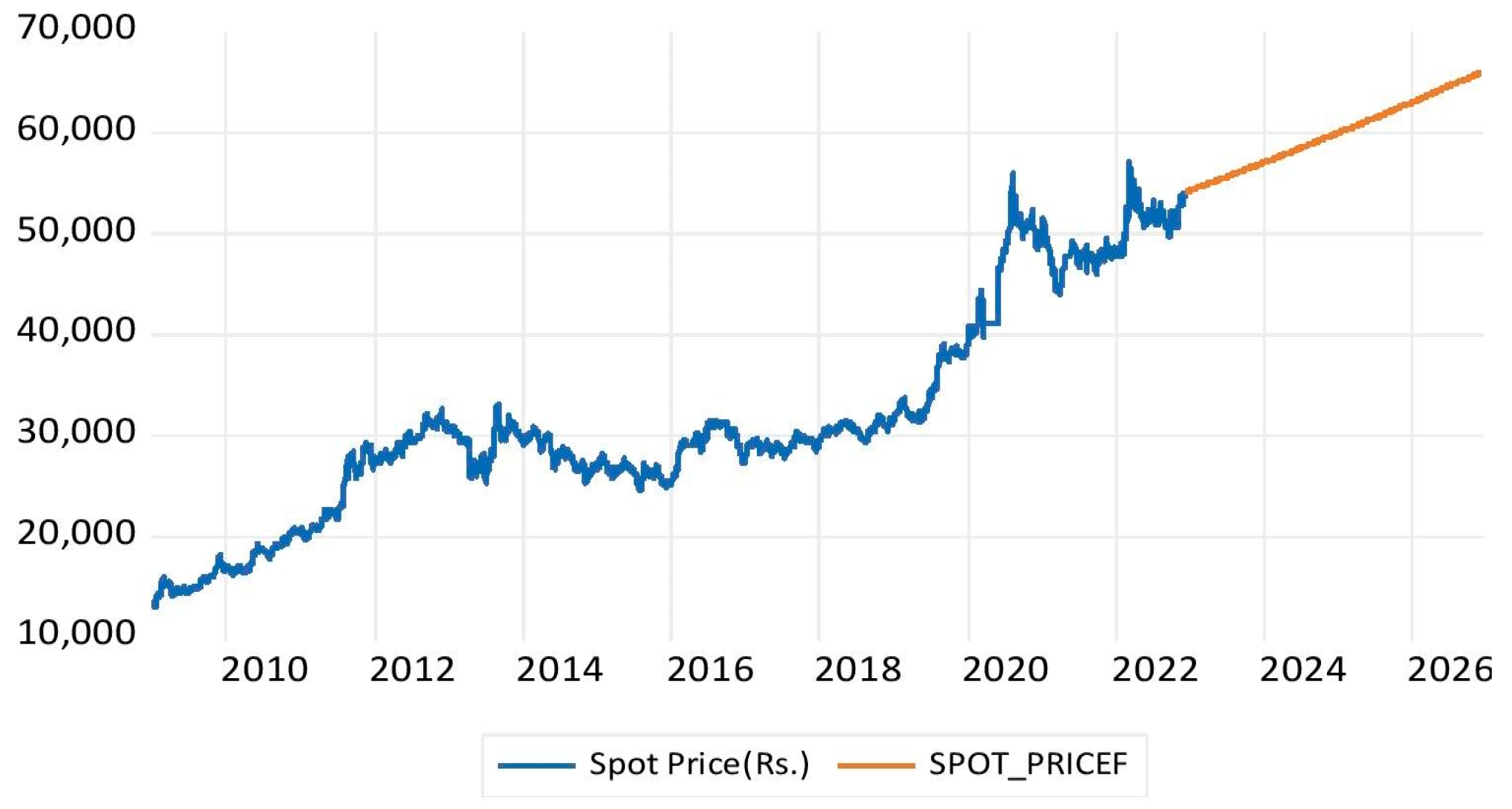
Recurrent stock market fall and rise sequel by COVID-19, rising global inflation, increase in Fed interest rates, the unprecedented meltdown of technology stocks, fear of trade wars, tightening of governments’ fiscal policies call for a new trend in international investing. It is time for the investors to rethink, rebalance and reset their investment strategies to position and protect their portfolios during and post-pandemic period. This paper attempts to forecast the gold prices for the post-pandemic era and explores whether gold will serve as a decisive hedge during this transition period. The techniques of ARCH, GARCH, E-GARCH, A-PARCH, and GARCH-M is employed in forecasting the conditional volatility of gold spot price from Multi Commodity Exchange (MCX) of India. A total of 3631 observations were collected from the daily spot prices of gold from January 2009 to December 2022. The findings show that the gold prices in India are highly persistent similar to other emerging markets and that gold will remain a safe haven for investors and institutional investors in the post-pandemic period. This paper is the first of its kind to forecast gold prices for the post-pandemic period. The forecast price of 10-gram gold is expected to trade for 65,948 ₹ in the Indian MCX by 2026 if the gold prices behold its previous momentum. This forecast will help the investors to plan their portfolio diversification for the post-pandemic period.

1. Introduction

The unprecedented stock market crash globally sequel by the COVID-19 pandemic has created unbridled global fears on capital market investments. The slump of recent crude oil prices, trade, capital, technology and biological wars among the world’s largest economies, the proposed US Securities and Exchange Commission (SEC) legislation in delisting Chinese firms on US stock exchanges, expectation of change in Fed interest rates, meltdown of technology stocks all creates a state of perplexity in the future trend of stock market movements. Advanced and emerging economies worldwide are now striving hard to combat this systematic risk by revising their monetary and fiscal policies with a quest for economic recovery and normalization. The economic impact of COVID-19 on the emerging markets is exceptionally adverse, fueled by high poor and financially vulnerable population, weak public health care systems, lack of awareness and knowledge regarding spread and prevention. India, one of the emerging economies, is significantly disrupted by this global economic downturn.
The Indian financial market has responded to this uncertainty dramatically. At the same time, institutional investors and fund managers could maneuver this trauma, the hard-hit hammers on small retail investors. Indian retail investors are losing their confidence and are perplexed by whether the recent stock price reaction reflects their performance. It is time for the investors to rethink, rebalance and reset their investment strategies to position and protect their portfolios during and post-pandemic period. Gold serves as a safe haven for such retail investors who look for the best alternative investment to preserve their portfolio assets. Lessons from the global financial downturn in 2008–2009 and earlier credit crunches stress the importance of portfolio diversification by reallocating equity investments with gold as a powerful hedging tool during transitional periods. As a financial asset, gold has consistently shown positive price momentum has maintained its value and purchasing power even during inflationary periods.
This paper aims to forecast the gold price returns for the post-pandemic period using various forms of General Autoregressive Conditional Heteroscedastic (GARCH) models such as GARCH, Threshold GARCH (T-GARCH), Exponential GARCH(E-GARCH), Asymmetric power ARCH (A-PARCH), and GARCH- in Mean (GARCH-M). We utilize daily data, including five days trading spot price of 10-gram gold from June 2009 to September 2021. The spot price of gold was extracted from the MCX of India. The findings show that gold prices in India are highly persistent similar to other emerging markets.
The remaining section of this paper is structured as follows. In Section 2, we review the literature related to the Indian gold market and its relative importance in the Indian economic system, which provides the research background to this study. The following section includes the research methodology with subsections on data description, its preliminary diagnostic, empirical model employed. Section 4 provides the empirical results. Finally, the study concludes with social and practical implications and future scope in Section 5.

2. Literature Review

Prior literature has identified numerous reasons for the extensive demand for gold. First, gold can act as an inflation hedge, especially during crisis periods (Gokmenoglu and Fazlollahi 2015; He et al. 2020). Second, it can also be utilized as an alternative investment for stocks and hedge against currencies as it is considered a safe asset that involves no credit risk as central banks retain it. Third, gold can help to transmit monetary policy to the economic system (Liu and Su 2019). Overall, it can be a diversifying asset in a portfolio representing up to 30–50% of total portfolio value if interest-earning deposits are unavailable (Dey and Sampath 2018). In addition to these reasons, gold holds a significant position in India due to cultural and traditional demands at weddings and festivals.
There have been various studies conducted on the gold sector in India. The majority of these studies linked it with stock markets, currencies, oil prices, and silver. Empirical studies prove the standard view of an inverse relationship between stock prices and gold. (Singhal et al. 2019) find that gold price significantly impacts the stock market in the long run. In a similar context, Mishra et al. (2022) found that Granger causality exists from gold price to stock price. Jain and Biswal (2016) find that fall in gold prices can cause a fall in the Indian currency and stock market index. They also confirm that gold represents an investment asset class.
Nevertheless, during high volatile periods, the co-relationship between gold and stock prices can be contemplated as a time of co-movements due to dependence (Mroua and Trabelsi 2020). At this juncture, investors reallocating their portfolios by increasing the percentage of gold will yield risk-adjusted returns and preserve their portfolio values in the post-pandemic period. The findings indicate that gold returns are not related to Bombay stock market indices. Therefore, gold can be considered a diversification tool in portfolios. On the other hand, gold returns can forecast the future price movements of consumer durables and fast-moving consumer goods and oil & gas indices.
Gold and silver have been connected to each other as both are precious metals that are mainly used for passive investments. The profit out of them replies on the expectation that their prices will increase. Furthermore, silver can be considered as a substitute for gold as both metals follow arbitrage and low risk spread trading features (Lucey and Tully 2006). According to Pradhan et al. (2020) the stream of literature on silver and gold can be grouped in to three domains; first the price reactions of these metals to macroeconomic conditions, second, the forecasting of their prices, third, the relationship between the two metal prices. Mishra et al. (2019) investigated the dynamic relationship between gold and silver in the Indian market. They highlighted the weak efficient form of the Indian market that calls for optimal decisions regarding portfolio investment and hedging. The study found a unidirectional relationship between gold and silver using rolling window bootstrap approach. However, Pradhan et al. (2020) show a mixed result of causality between silver and gold. Su et al. (2020) and Qin et al. (2020) indicated the significance of capturing the parameter instability in the analysis of gold and silver using Granger-causality approach. In a recent study, Sami (2021) examines the cointegrating relationship between gold and silver prices in India. The results reveal a significant cointegrating long-run relationship between the two metals.
Dey and Sampath (2020), while investigating the spillover of five major asset classes in India, find a paradigm shift in the dynamics of gold’s impact on the Indian economy post demonetization. The study highlights the emergence of IT sector as a critical mediator between the gold and the rupee-dollar exchange rate markets in India. Indeed, any form of economic reform impacts the gold prices in India. Kumar and Maheswaran (2013) found a positive, long-run volatility spillover effect of crude oil on the commodities market. However, Rastogi et al. (2021), did not find any evidence of gold and crude oil volatility spillover on interest rates. Nevertheless, the price variations in gold and crude oil impact the economy but do not adversely affect interest rates.
During the pandemic, several papers have examined whether gold is a safe-haven asset or not. The findings of these papers were mixed; for instance, (Ji et al. 2020) and (Salisu et al. 2021) have evinced that gold has proven to be a safe-haven asset against equity returns and oil price risks, respectively. On the other hand, Cheema et al. (2022) indicate contradicting results. Using thirteen Asian stock market data, Yousaf et al. (2021) find supportive results for the role of gold as a solid safe-haven asset in China, Indonesia, Singapore, and Vietnam, and a weak safe-haven in Pakistan and Thailand. Gharib et al. (2021) show a bilateral contagion impact of bubbles in the oil and gold market during COVID-19. However, the above-mentioned empirical studies focused on the gold performance during the pandemic; we attempt to forecast the gold prices for the post-pandemic era in India, one of the largest importers of gold globally.

Indian Gold Market

The official gold imports of India in Feb 2021 recorded its highest in the Indian gold import history of 165 tons (approx.). Multiple factors attribute to this ever-rising gold imports in India. Rising income levels of the middle-class Indian population and increasing gold prices are considered to be major long-run drivers of this affluent demand for gold at the macro level. Inflation and gold price changes also trigger gold demand in the short run. Additionally, the perception of the Indian population about this precious metal has a central role to play. Among the Indian middle-class population, gold is mainly perceived as a symbol of wealth, social status, and secured investment with high liquidity.
Furthermore, gold holds a significant position in India due to its cultural background and traditional demands at weddings and festivals. These factors have made India a global leader in consuming gold jewelry, bar, and coins for decades. In addition, the sharp decline in bank interest rates in the recent past further increases investors’ preference for gold investments. Gold has various investment instruments in India, such as gold ETFs, bullion, gold sovereign bonds, and gold mutual funds traded in the multi-commodity exchange market.

3. Discussion

3.1. Sample Data

This paper employs daily data of gold spot price during the period from January 2009 to December 2022. A total of 3631 observations including the five-day trading price of 10-gram gold was sourced from the MCX of India. The spot price is denominated in Indian currency which possess an absolute value we converted the price into return series. Systematic research always calls for converting absolute values to a return series, which likely to have constant means and variance over the sample period (Kumar and Maheswaran 2013). Therefore, the gold return is calculated as a proportion of the natural log of the spot price over a one-day lagged price. Rit = log (Pit/Pi,t−1), where Rit = the return of the asset i at time t, Pit is the asset i at t time, and Pt−1 is the price of asset i at one lagged period t−1.

3.2. Preliminary Diagnostics

As we use time-series data in this research paper, it is highly imperative to run the preliminary diagnosis of the data to avoid spurious results and to report better forecasting models. The preliminary diagnosis in time series includes the test for stationarity, autocorrelation, and white noise (Agung 2011; Meister and Kreiß 2016) which have been discussed in detail below.

3.2.1. Stationarity

One of the critical assumptions to apply to forecasting models is that the time series data must be stationary to generalize the results to other periods. A time series is considered stationary if its mean and covariance are constant over time (Gujarati 2011). Employing non-stationary times series data in financial models draws unreliable and spurious forecasting results. The Augmented Dickey-Fuller (ADF) test considered as a spurious test in examining the unit root in any series tests the following regression with three assumptions
ΔYt = α + βt + δYt−1 + γ1Yt−2 + γ2Yt−3 + εt
where α includes intercept assumption, β holds trend assumption, and δ augments unit root assumption wherein γ1Yt−2 + γ2Yt−3 are the lagged values that can be selected using SIC criteria generally with a maximum lag length of 24.

3.2.2. Autocorrelation

Attribute to the correlation of a financial time series amidst its previous (lagged) values, and the partial autocorrelation (PACF) shows the correlation between the current observation (yt) with its own previous lagged values (k) while controlling the intermediate lags. In other terms it shows the correlation between yt and yt − k, subsequently excluding the effects of yt−k+1, yt−k+2, , yt−1. The presence of autocorrelation and PACF in the return series is examined using correlogram and Breusch Godfrey serial correlation LM test.
Additionally, researchers have documented that the presence of so-called “stylized facts” in financial and economic series is ubiquitous for large datasets with high-frequency observations like daily prices. As our data set includes 3631 observations which can be considered as a large data set, we examine the presence of the stylized facts include volatility clustering, leptokurtic of marginal distributions, mean reversion, and financial series asymmetries (Meister and Kreiß 2016; Teräsvirta 2009) in sample data.

3.2.3. Volatility Clustering

In developing forecasting models in time series data, the mean equation takes the common form of
Yt = α + β1Yt−1 + β2Et−1 + εt
where, β1Yt−1 + β2Et−1 is the predicted value. Based on this Yt value the residual error term will be equal to
Et = YtŶt
where, Yt = actual or realized value Ŷt is the predicted value. In employing predictive modeling techniques with time-series data, it is imperative to identify whether the error term (Et) of the forecasting equation is white noise or not. White noise indicates that the residuals are random with no patterns. The critical assumptions of white noise include zero mean residuals, constant variance in error terms, and normal distribution of residuals. In computing Yt, the error terms of the mean equation may not have constant variance, which contradicts the stationary and homoscedastic distribution of error terms. The error terms may be very high at times, generally known as a highly volatile period followed by a stable period where error term values are low. The behavior pattern of error terms that showcase the appearance of large absolute returns (Et) in financial assets group together is commonly called volatility clustering. The presence of volatility clustering in the financial rate of return series strongly depicts that the volatility encompasses a certain degree of interdependence of its historical values. In other words, the current volatility level positively correlates with its immediate prior term (Brooks 2008). The presence of volatility clustering in the residuals could be visually captured using a residual graph, and an Autoregressive Conditional Heteroscedasticity (ARCH) test can be performed to substantiate the presence of autoregressive conditional heteroscedasticity in the residuals.

3.2.4. Leptokurtic Distribution

An empirical distribution of daily data tends to have conditional distribution sharply spiked at zero with fat tails is commonly named as leptokurtic distribution. Kurtosis coefficient measures leptokurtosis as a ratio of the sample fourth-order moment to the squared sample variance (Francq and Zakoian 2020). Histogram plots are used to examine whether the series possesses leptokurtic distribution that has fat tails or not.

3.3. Empirical Model

The General Autoregressive Conditional Heteroskedasticity (GARCH), developed by (Bollerslev 1986), is a renowned forecasting model that can accommodate and explain the stylized facts of financial time series. Prior literature has also evidenced that leptokurtic asymmetric distributions have proven better forecasting ability with GARCH models (Li et al. 2013; Wilhelmsson 2006). The GARCH models parametrize the autocorrelation in volatility by allowing the conditional variance of the error terms to depend on its lagged squared error (Brooks 2008). The conditional variance equation can be written as
σ t 2 = ω + i = 1 q α i ε t i 2 + i = 1 p β i σ t i 2
A simple form of GARCH (1,1) takes the following form
σ t 2 = ω 0 + α 1 ε t 1 2 + β 1 σ t 1 2
σ2 is the conditional variance to be forecasted based on past information, α 1 ε t 1 2 is the information about volatility from previous lag, and σ t 1 2 is the fitted variance from previous lag, ω is the constant term, α and β are ARCH and GARCH coefficient terms.
In GARCH models, the conditional variance indicated as a linear function of squared lagged values tends to explicitly captures the so-called stylized facts in financial time series. More specifically, GARCH (1,1) having three variables in the conditional variance have higher order capability in obtaining a good model especially for financial series commodity market data. Apparently, as reported by previous papers, it is strenuous to identify a model that surpass the classical GARCH (1,1) where p = 1 (1 lag variance) and q = 1 (1 lag of residual error) (Hansen and Lunde 2006). We also found compelling evidences substantiate that GARCH (1,1) model with only three parameters have proven its unbiases in its predictive
We also found compelling evidences substantiate that GARCH (1,1) model with only three parameters have proven its unbiases in its predictive ability exceptionally in commodity markets (Čermák et al. 2017; Handika and Chalid 2018; Trabelsi et al. 2021) and in forecasting stock price volatility (Hansen and Lunde 2006; Jain and Biswal 2016; Sharma 2015). However, in some cases, the model may improve to capture the series dynamics, especially the asymmetric volatility, which can be captured by TGARCH, EGARCH, PGARCH, and APARCH models. GARCH-M attempts to estimate the relationship between risk and returns in the gold return series.

4. Results and Discussion

This section summarizes the results of descriptive statistics of the data set, pre diagnostic test results, selection of GARCH model, residual and coefficient diagnostics of the proposed model and the forecasting of future gold prices.

4.1. Descriptive Statistics

Table 1 shows the descriptive statistics of the spot price and percentage returns of gold. The mean returns of daily price of gold are 31,321.15 ₹ and gold returns is 0.038% which are all positive and significantly vary from zero. This average positive return looks promising for retail investors in a country that ranks top in gold jewelry consumption. This substantiates the fact that gold has proven to be a safe haven for investors to hedge their portfolio risk. Over the sample period the gold returns had reached its apex rate of 12% with a lowest margin of −8% which clearly depicts the heighten volatility of this precious yellow metal. The kurtosis of gold price returns exhibits leptokurtic distribution (with fat tails) of our time series data which is one the stylized facts to employ GARCH models.

4.2. Preliminary Diagnostics Results

Preliminary screening of the sample data is indispensable in time series modeling. The stationary of the data series must be confirmed to avoid spurious regression results in the forecasting models. Subsequently the optimal lag order is selected from autocorrelation and partial autocorrelation tests of the mean equation. Finally, the presence of ARCH effects in the residuals is confirmed to proceed with the application GARCH model.

4.3. Stationarity Results of Gold Spot Price

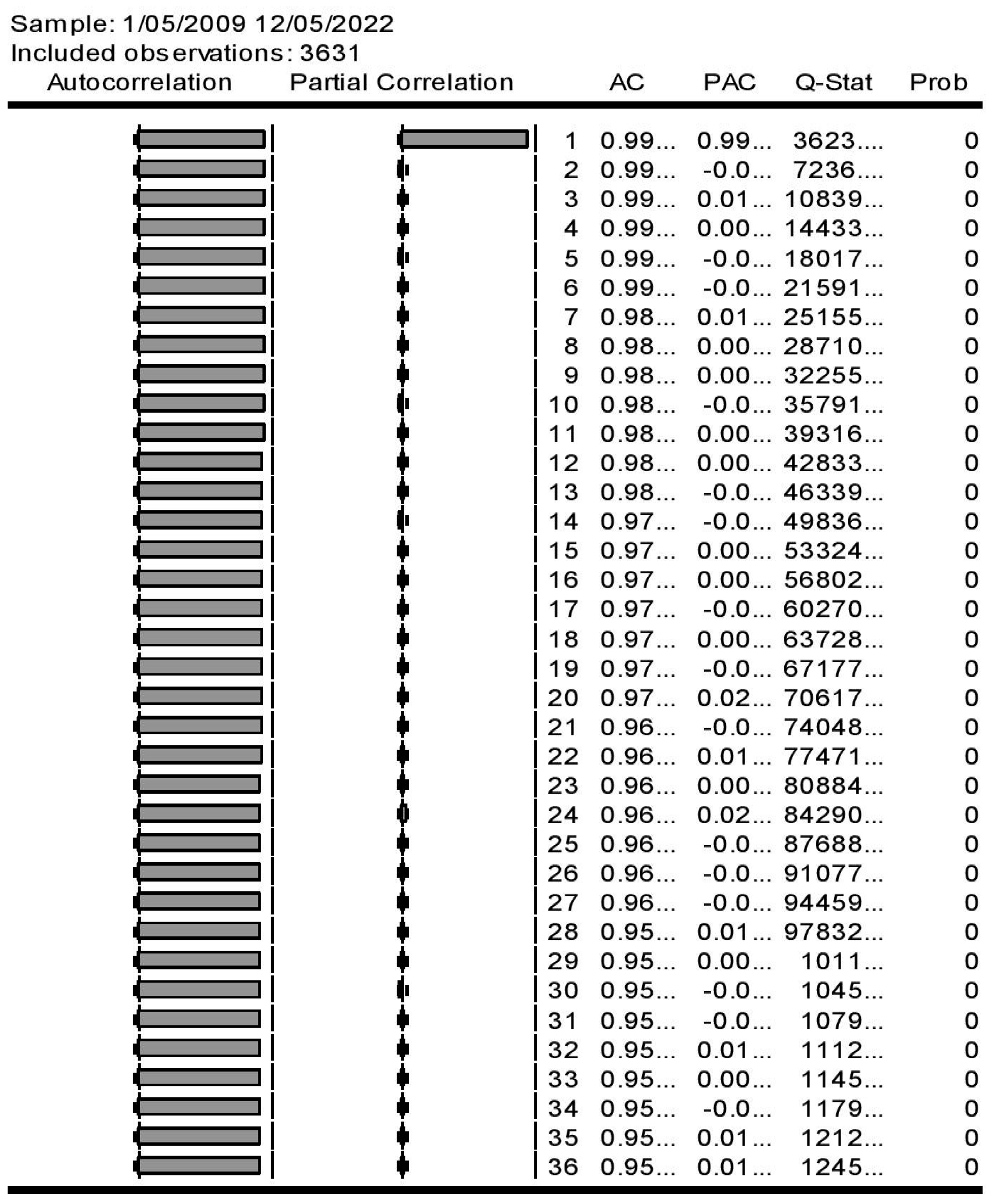
Though a trivial volatility in gold prices is observed from Figure 1, there is a marginal increase in the price of this yellow metal continuously increases over two decades. Figure 1 captures the record-breaking trading price of gold at its peak during the COVID 19 pandemic outbreak in 2020. The stationarity of the gold price series is initially examined through graphical representation (Figure 1), correlogram (Figure 2), and unit root test using the ADF test by employing Equation (1). Figure 1 indicates that the gold price series is non-stationary as it is drifting upwards with fair heaps of variations.
As a further step in examining the stationarity of gold series we examined the correlogram plot of gold price to audit the Auto-Correlation (AC) and Partial Auto-Correlation (PAC) values and the results are presented in Figure 2. Figure 2 reports a high correlation of about 0.95 between current gold price and lagged gold price even up to 36 days. In addition, the estimated autocorrelation (AC) is also slowly declining. The marginal decrease in the AC values, and the highest insignificant value of the first PAC and the significant p values of the 36 lags of the gold series clearly depicts that the series is non-stationary.
Subsequently, the unit root test was performed using the ADF test to check the stationarity of the gold spot price series. The ADF results is presented in Table 2 shows that the presence of unit root in gold prices and thus the null hypothesis is accepted.
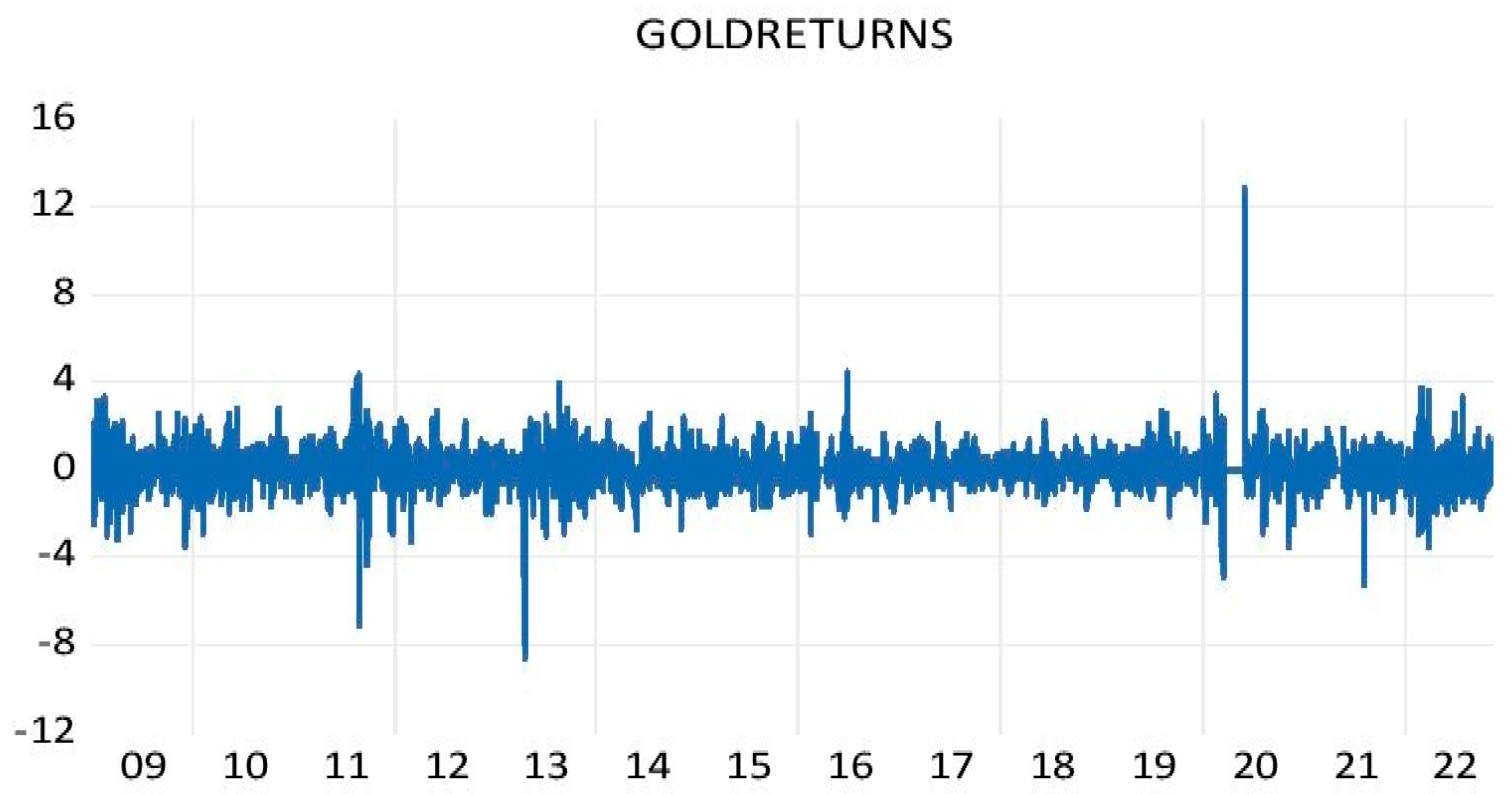
In order to transform the gold series to stationary the returns of gold prices are computed by taking the natural log of daily price with its one previous lagged value and the process of unit root test is repeated. Figure 3 showcase the gold returns evidences the presence of volatility clustering in the series, large changes followed by large changes and small changes come after small changes in return series. The exhibit of mean reversion in the gold returns indicates that the series is stationary.
The ADF test is repeated for gold returns to statistically prove that the series is stationary at level (Table 3). The ADF test results show that the coefficient of gold returns is highly significant at 0.000 level. This confirms the rejection of the null hypothesis and the acceptance of the alternative hypothesis that the series is stationary to proceed with the further critical assumptions of forecasting models.
As a further step, we developed a mean equation with constant as independent variable and observed the AC and PAC values of correlogram had a significant spike at lags 1, 4, 5 and 9. Subsequently we modified the mean equation by including AR terms. The estimated mean equation includes gold spot price as dependent variable regressed with lagged values and a constant term using Least Squares (LS) and Autoregressive Moving Average model (NLS and ARMA) methods. Table 4 shows the results of the mean equation.
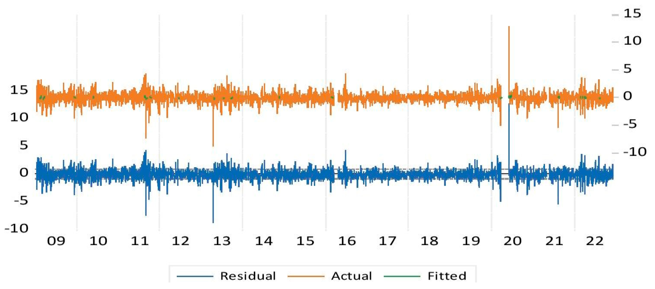
The D-W value close to 2 in the mean equation indicates the presence of no autocorrelation in the residual series. In examining the model fit of the above equation we applied the residual diagnostics test of correlogram by creating a residual series ‘RESID 01’ exhibited in Figure 4.
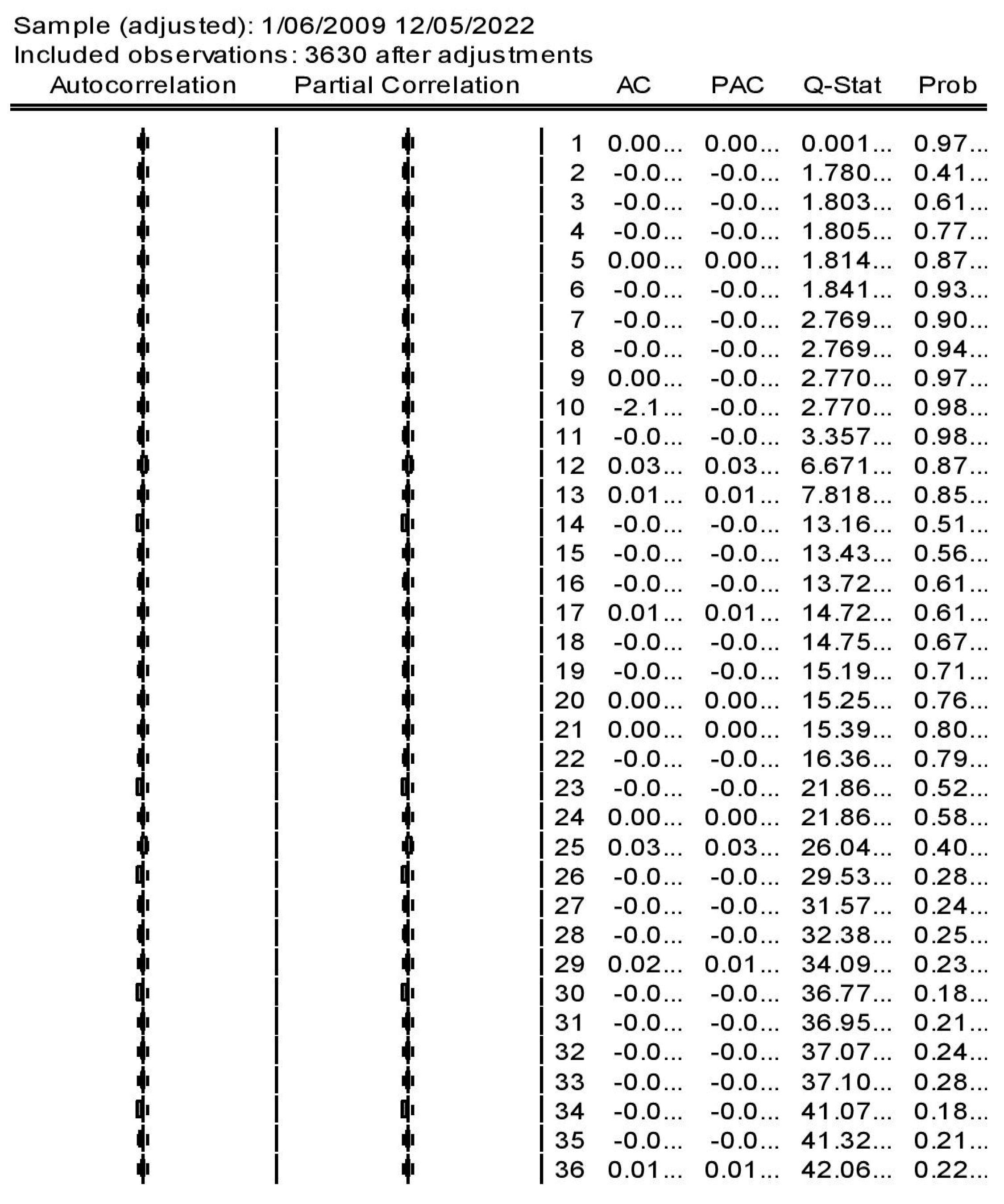
The highest volatility in gold price residuals is captured in the month of July when the number of confirmed cases of COVID-19 cases reached 1 million. The residual graph of LS regression also shows signs of significant volatility clustering which is imperative in applying GARCH models. Indeed, the correlogram plot of the residual series in Figure 5 with no significant spikes support that the error terms are white noise.
Additionally, the unit root test for the residual series as shown in Table 5 confirms that the residuals are stationary as the p values are less than 0.05. To sum up, we can conclude that the residual diagnostics clearly indicate that the mean equation is correctly specified.
As a continuation of the preliminary analysis, the conditional heteroscedasticity was tested using formal volatility test of autoregressive conditional heteroscedasticity (ARCH) and the results are presented in Table 6. The F-statistics is 8.79 and the p-value less than 0.05 augment the presence of ARCH effect which indicate the presence of significant volatility clustering in the residuals. Consequently, the presence of significant ARCH effect in the residuals green signals the appropriateness of applying univariate GARCH framework in gold returns series.

4.4. Empirical Model Results

Table 7 presents the mean and conditional volatility equations of ARCH, GARCH, TGARCH, E-GARCH, A-PARCH, and GARCH-M techniques in forecasting the conditional volatility of gold spot price from the Indian commodity market. We have selected the model based on the three selection criteria Akaike Information Criterion (AIC), Schwarz Criterion (SC), and Hannan Quinn (HQ) Criterion. Based on the model selection indicators, we considered three models: EGARCH, APARCH, and TGARCH, which capture the asymmetric volatility of gold returns. The unusual insignificant (5% level) negative outcome of leverage parameter in TARCH, A-PARCH and EGARCH models prompted us to select the GARCH (1,1) model. Table 7 shows that the estimated power coefficients are significantly different from 1 or 2, which strongly evidences the inability to reject Bollerslev formulation and support the GARCH model as appropriate in modeling gold return series. Finally, we selected GARCH (1,1) model where p = 1 and q = 1 as the best fit. The coefficient of lagged squared residual and lagged conditional variance in the conditional variance equation both are highly statistically significant in our model.
Gold is often substantiated as a safe haven asset to hedge inflation, other currencies, stocks market shocks during economic uncertainties for Indian investors. Consequently, the investment in gold is driven by these factors and not in all cases by the price changes in the asset (Dey and Sampath 2018) Unlike stock market reactions which are short lived, investor’s reaction to gold price changes has momentum effect. Apparently, we find that applying a symmetric model (GARCH) to forecast the gold prices is relevant.
In a common form of the GARCH model, the sum of the coefficients on the lagged squared error and the lagged conditional variance is approximately near to 1 (Brooks 2008). In our conditional variance equation, we found that the coefficient of α is 0.149 and β is 0.599, and the sum of ARCH and GARCH terms equals 0.75. The decaying rate of the volatility i 0.25. The higher value of β compared to α implies that shocks to the condition-al variance of gold returns in the Indian commodity market are highly persistent. The persistence volatility shocks indicate that the gold prices fluctuations, once started, may take a longer time to return to a quieter phase. Similar results on gold prices were reported by Cao et al. (2015) on the Chinese market, Ping et al. (2013) from the Malaysian market, Sopipan et al. (2012), from London, and Irene et al. (2020) findings on world gold prices.

4.5. Residual Diagnostics of the Empirical Model

This section presents the validity and the model fit, including residual and coefficient diagnostics. Firstly ARCH_LM test was applied to assess the presence of heteroskedasticity in the residual series of the GARCH model. The results are presented in Table 8.
The F statistic at 0.092139 supports the acceptance of the null hypothesis, proving that there is no serial correlation in the residuals series. The correlogram plot reassured the results of the ARCH LM test of the squared residuals. Figure 6 clearly indicates that the error terms are white noise as the PAC and AC values in the plot lie within the 5% significance limits. Furthermore, the p values of Q-stat remain insignificant till lag 36.

4.6. Engle-Ng Sign-Bias Test

Engle -Ng tests validate whether an asymmetric or symmetric model to be applied. The test also examines the impact of positive and negative returns shocks on volatility not captured by our proposed model. Table 9 shows the result of the Engle-Ng Sign Bias test. The sign-bias, negative, positive, and joint bias insignificant t-stat values highlight that there is no leverage effect present in the standardized residuals. The results validate that our symmetric model is deemed adequate.

4.7. Coefficient Diagnostics of the Empirical Model

To test the stability of the parameters of the model, we use the nyblom parameter stability test. This test assesses the variance of the parameters included in our model. From the results of this test static, as shown in Table 10, we confirm that our parameters are stable and do not shift over time.

4.8. Forecasting of Gold Price Using Empirical Model

In forecasting the conditional volatility of gold prices for the next five years, we increased the sample size by adding 1044 observations to the actual sample of 3631 observations. Then, in the mean equation estimates, we applied GARCH (1,1) and forecasted the gold price for the next five years till December 2026, as shown in Figure 7. Thus, SPOT_PRICE indicates the historical price, and SPOT_PRICEF signifies the forecast of future gold price. To conclude, if India’s gold prices follow its previous momentum, we expect that the price of 10-gram gold in the Indian commodity market will reach 54,236 ₹ by 2023 and 65,948 ₹ by 2026 based on our model estimates.

5. Conclusions

5.1. Conclusion

The global economic downturn and the significant decline in stock market crash fueled by the COVID 19 affect investors’ expectations and planned behavior. Indian stock market index NIFTY 500 recorded −0.112% returns in 1st January 2020, −24% in 1st March 2020, +6% in July 2020 and −1.8% in 31st January 2021, and +1.4% in August 2021, creating uncertainty about future returns compels investors to reallocate their portfolio to preserve their assets in the portfolio. Strong evidence shows that gold bestows a decisive hedge over equity investment and is often negatively correlated during risk-on periods (Bouri et al. 2017; Jain and Biswal 2016). The long-run gold prices suggest that India’s gold prices are continuously increasing ever since 2009. Especially the performance of gold has been solid over the recent decades, driven by key structural changes in the Indian economy. The average annual return of gold was 9.10% in the last ten years, increased to 14.70% in the last five years, and outperformed other portfolio components by securing 24.34% in the last two years of the pandemic as against 16.41% of S&P BSE Sensex. Driven by many micro and macro factors that affect gold prices in India, a question is raised on whether it will remain a safe haven for investors in the post-pandemic period. This paper tries to model the volatility of gold prices from the Indian commodity market and forecast the spot gold prices for the next five years using the univariate GARCH (1,1) model. The results show that the gold prices in India are highly persistent like other emerging markets. We can conclude that the reason for gold prices volatility in the Indian market is due to its persistence.

5.2. Practical Implication

As a part of implication, this paper forecasts that the price of 10-gram gold is expected to be traded for 65,948 ₹ in the Indian MCX by 2026 if the gold prices behold its previous momentum. This gives a practical implication that gold will remain a safe haven for investors and institutional investors in the post-pandemic period. The findings shed light for the policymakers and regulators on the impact of the pandemic on one of the most important financial assets in India. Gold prices are affected by the government decisions, and macroeconomic conditions and hence have experienced a high increase in its price level; therefore, as chances of formation of price bubble increase, policymakers should be cautious to avoid a boom-bust cycle in the post-pandemic period (Akhtaruzzaman et al. 2021).

5.3. Limitations and Future Research Directions

Although we strive our best in presenting quality research work, this study also has limitations. The scope of this study is confined only to the Indian market, and the results might provide better insights to investors from emerging economies; however, the results may vary. Additionally, our estimates of gold future prices are computed based on the historical prices that any economic uncertainties or events may surpass this forecast. In addition, we have used the univariate GARCH model in forecasting future prices. Future research directions may include applying Multivariate GARCH models, including the micro and macroeconomic variables that drive the demand for gold in other developed or developing economies.

Author Contributions

S.K. and Y.A formulated the study design. Y.A. designed and conceived the research methodology. S.K. and S.K.P. collected and formulated the data as per the software requirement. S.K. analyzed and interpreted the data. S.K., Y.A. and S.K.P. finalized the paper. S.K.P. formatted and proofread the paper. All authors have read and agreed to the published version of the manuscript.

Funding

The authors confirm that there is no funding support from any source for this research work.

Data Availability Statement

The dataset will be provided upon request.

Conflicts of Interest

The authors declare no conflict of interest.

References

  1. Agung, Gusti Ngurah. 2011. Time Series Data Analysis Using EViews. Singapore: John Wiley & Sons. [Google Scholar]
  2. Akhtaruzzaman, Md, Sabri Boubaker, Brian M. Lucey, and Ahmet Sensoy. 2021. Is gold a hedge or a safe-haven asset in the COVID–19 crisis? Economic Modelling 102: 105588. [Google Scholar] [CrossRef]
  3. Bollerslev, Tim. 1986. Generalized autoregressive conditional heteroskedasticity. Journal of Econometrics 31: 307–27. [Google Scholar] [CrossRef] [Green Version]
  4. Bouri, Elie, Anshul Jain, Pratap Chandra Biswal, and David Roubaud. 2017. Cointegration and nonlinear causality amongst gold, oil, and the Indian stock market: Evidence from implied volatility indices. Resources Policy 52: 201–6. [Google Scholar] [CrossRef]
  5. Brooks, Chris. 2008. RATS Handbook to Accompany Introductory Econometrics for Finance. Cambridge: Cambridge University Press. [Google Scholar]
  6. Cao, Guangxi, Yingchao Zhao, and Yan Han. 2015. Asymmetric statistical features of the Chinese domestic and international gold price fluctuation. International Journal of Modern Physics B 29: 1550113. [Google Scholar] [CrossRef]
  7. Čermák, Michal, Karel Malec, and Mansoor Maitah. 2017. Price Volatility Modelling–Wheat: GARCH Model Application. AGRIS On-Line Papers in Economics and Informatics 9: 15–24. [Google Scholar] [CrossRef] [Green Version]
  8. Cheema, Muhammad A., Robert Faff, and Kenneth R. Szulczyk. 2022. The 2008 global financial crisis and COVID-19 pandemic: How safe are the safe haven assets? International Review of Financial Analysis 83: 102316. [Google Scholar] [CrossRef]
  9. Dey, Shubhasis, and Aravind Sampath. 2020. Returns, volatility and spillover–A paradigm shift in India? The North American Journal of Economics and Finance 52: 101110. [Google Scholar] [CrossRef]
  10. Dey, Shubhasis, and Aravind Sampath. 2018. Dynamic linkages between gold and equity prices: Evidence from Indian financial services and information technology companies. Finance Research Letters 25: 41–6. [Google Scholar] [CrossRef]
  11. Francq, Christian, and Jean-Michel Zakoian. 2020. Virtual Historical Simulation for estimating the conditional VaR of large portfolios. Journal of Econometrics 217: 356–80. [Google Scholar] [CrossRef] [Green Version]
  12. Gharib, Cheima, Salma Mefteh-Wali, and Sami Ben Jabeur. 2021. The bubble contagion effect of COVID-19 outbreak: Evidence from crude oil and gold markets. Finance Research Letters 38: 101703. [Google Scholar] [CrossRef]
  13. Gokmenoglu, Korhan, and Negar Fazlollahi. 2015. The interactions among gold, oil, and stock market: Evidence from S&P500. Procedia Economics and Finance 25: 478–88. [Google Scholar]
  14. Gujarati, Damodar. 2011. Econometrics by Example. New York: Palgrave Macmillan, vol. 1. [Google Scholar]
  15. Handika, Rangga, and Dony Abdul Chalid. 2018. The predictive power of log-likelihood of GARCH volatility. Review of Accounting and Finance 17: 482–97. [Google Scholar] [CrossRef]
  16. Hansen, Peter Reinhard, and Asger Lunde. 2006. Consistent ranking of volatility models. Journal of Econometrics 131: 97–121. [Google Scholar] [CrossRef]
  17. He, Xie, Tetsuya Takiguchi, Tadahiro Nakajima, and Shigeyuki Hamori. 2020. Spillover effects between energies, gold, and stock: The United States versus China. Energy & Environment 31: 1416–47. [Google Scholar] [CrossRef]
  18. Irene, Yanne, Madona Yunita Wijaya, and Aisyah Muhayani. 2020. World Gold Price Forecast using APARCH, EGARCH and TGARCH Model. InPrime: Indonesian Journal of Pure and Applied Mathematics 2: 71–78. [Google Scholar] [CrossRef]
  19. Jain, Anshul, and Pratap Chandra Biswal. 2016. Dynamic linkages among oil price, gold price, exchange rate, and stock market in India. Resources Policy 49: 179–85. [Google Scholar] [CrossRef]
  20. Ji, Qiang, Dayong Zhang, and Yuqian Zhao. 2020. Searching for safe-haven assets during the COVID-19 pandemic. International Review of Financial Analysis 71: 101526. [Google Scholar] [CrossRef]
  21. Kumar, Dilip, and S. Maheswaran. 2013. Correlation transmission between crude oil and Indian markets. South Asian Journal of Global Business Research 2: 211–29. [Google Scholar] [CrossRef]
  22. Li, Yong, Wei-Ping Huang, and Jie Zhang. 2013. Forecasting volatility in the Chinese stock market under model uncertainty. Economic Modelling 35: 231–34. [Google Scholar] [CrossRef]
  23. Liu, Guo-Dong, and Chi-Wei Su. 2019. The dynamic causality between gold and silver prices in China market: A rolling window bootstrap approach. Finance Research Letters 28: 101–6. [Google Scholar] [CrossRef]
  24. Lucey, Brian M., and Edel Tully. 2006. The evolving relationship between gold and silver 1978–2002: Evidence from a dynamic cointegration analysis: A note. Applied Financial Economics Letters 2: 47–53. [Google Scholar] [CrossRef]
  25. Meister, Alexander, and Jens-Peter Kreiß. 2016. Statistical inference for nonparametric GARCH models. Stochastic Processes and Their Applications 126: 3009–40. [Google Scholar] [CrossRef]
  26. Mishra, Bibhuti Ranjan, Ashis Kumar Pradhan, Aviral Kumar Tiwari, and Muhammad Shahbaz. 2019. The dynamic causality between gold and silver prices in India: Evidence using time-varying and non-linear approaches. Resources Policy 62: 66–76. [Google Scholar] [CrossRef]
  27. Mishra, Ashwini Kumar, Kshitish Ghate, Jayashree Renganathan, Joushita Kennet, and Nilay Pradeep Rajderkar. 2022. Rolling, recursive evolving and asymmetric causality between crude oil and gold prices: Evidence from an emerging market. Resources Policy 75: 102474. [Google Scholar] [CrossRef]
  28. Mroua, Mourad, and Lotfi Trabelsi. 2020. Causality and dynamic relationships between exchange rate and stock market indices in BRICS countries: Panel/GMM and ARDL analyses. Journal of Economics, Finance and Administrative Science 25: 395–412. [Google Scholar] [CrossRef]
  29. Ping, Pung Yean, Nor Hamizah Miswan, and Maizah Hura Ahmad. 2013. Forecasting Malaysian gold using GARCH model. Applied Mathematical Sciences 7: 2879–84. [Google Scholar] [CrossRef]
  30. Pradhan, Ashis Kumar, Bibhuti Ranjan Mishra, Aviral Kumar Tiwari, and Shawkat Hammoudeh. 2020. Macroeconomic factors and frequency domain causality between gold and silver returns in India. Resources Policy 68: 101744. [Google Scholar] [CrossRef] [PubMed]
  31. Qin, Meng, Chi-Wei Su, Ran Tao, and Muhammad Umar. 2020. Is factionalism a push for gold price? Resources Policy 67: 101679. [Google Scholar] [CrossRef]
  32. Rastogi, Shailesh, Adesh Doifode, Jagjeevan Kanoujiya, and Satyendra Pratap Singh. 2021. Volatility integration of gold and crude oil prices with the interest rates in India. South Asian Journal of Business Studies. [Google Scholar] [CrossRef]
  33. Salisu, Afees A., Xuan Vinh Vo, and Adedoyin Lawal. 2021. Hedging oil price risk with gold during COVID-19 pandemic. Resources Policy 70: 101897. [Google Scholar] [CrossRef]
  34. Sami, Janesh. 2021. Has the long-run relationship between gold and silver prices really disappeared? Evidence from an emerging market. Resources Policy 74: 102292. [Google Scholar] [CrossRef]
  35. Sharma, Prateek. 2015. Forecasting stock index volatility with GARCH models: International evidence. Studies in Economics and Finance 32: 445–63. [Google Scholar] [CrossRef]
  36. Singhal, Shelly, Sangita Choudhary, and Pratap Chandra Biswal. 2019. Return and volatility linkages among International crude oil price, gold price, exchange rate and stock markets: Evidence from Mexico. Resources Policy 60: 255–61. [Google Scholar] [CrossRef]
  37. Sopipan, Nop, Pairote Sattayatham, and Bhusana Premanode. 2012. Forecasting volatility of gold price using markov regime switching and trading strategy. Journal of Mathematical Finance 2: 121. [Google Scholar] [CrossRef] [Green Version]
  38. Su, Chi-Wei, Meng Qin, Ran Tao, and Xiaoyan Zhang. 2020. Is the Status of Gold Threatened by Bitcoin. Ekonomska Istrazivanja-Economic Research 33: 420–37. [Google Scholar] [CrossRef]
  39. Teräsvirta, Timo. 2009. An introduction to univariate GARCH models. In Handbook of Financial Time Series. Berlin and Heidelberg: Springer, pp. 17–42. [Google Scholar]
  40. Trabelsi, Nader, Giray Gozgor, Aviral Kumar Tiwari, and Shawkat Hammoudeh. 2021. Effects of price of gold on Bombay stock exchange sectoral indices: New evidence for portfolio risk management. Research in International Business and Finance 55: 101316. [Google Scholar] [CrossRef]
  41. Wilhelmsson, Anders. 2006. GARCH forecasting performance under different distribution assumptions. Journal of Forecasting 25: 561–78. [Google Scholar] [CrossRef] [Green Version]
  42. Yousaf, Imran, Elie Bouri, Shoaib Ali, and Nehme Azoury. 2021. Gold against asian stock markets during the COVID-19 outbreak. Journal of Risk and Financial Management 14: 186. [Google Scholar] [CrossRef]
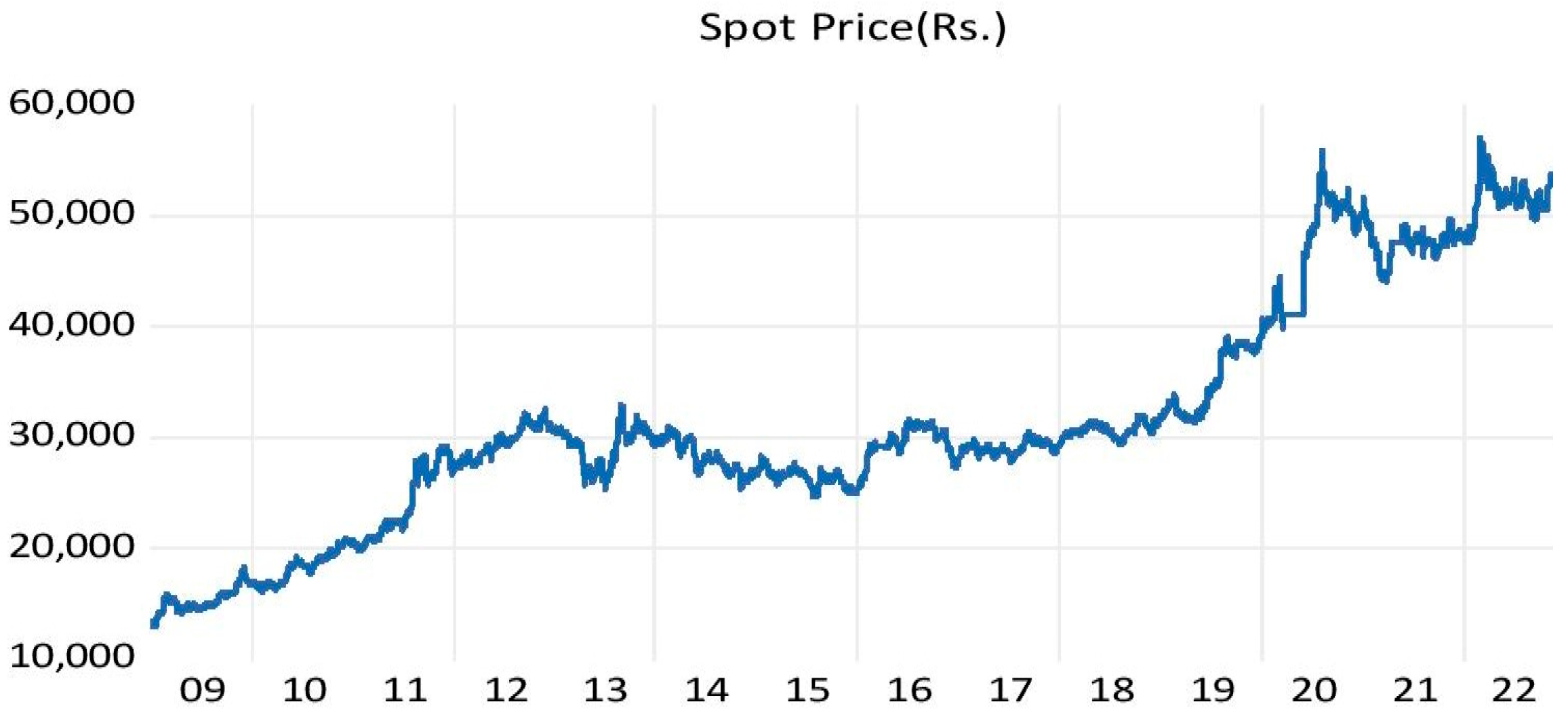
Figure 1. Gold Spot price.
Ijfs 11 00008 g001
Figure 2. Correlogram Plot of Gold Price.
Ijfs 11 00008 g002
Figure 3. Gold Returns.
Ijfs 11 00008 g003
Figure 4. Actual, Fitted, Residual Graph of OLS Regression on Gold Price Returns.
Ijfs 11 00008 g004
Figure 5. Correlogram plot of Residual series.
Ijfs 11 00008 g005
Figure 6. Correlogram plot of Squared Residuals. * indicates significant probability levels.
Ijfs 11 00008 g006
Figure 7. Gold Price Forecast for 2026.
Ijfs 11 00008 g007
Table 1. Descriptive Statistics.
ParameterSPOT_PRICEGOLD RETURNS
Mean31,321.150.038384
Median29,442.000.000000
Maximum57,006.0012.84899
Minimum12,935.00−8.65765
Std. Dev.10,289.300.864064
Skewness0.6157760.465281
Kurtosis2.71300922.87019
Jarque-Bera241.928159,848.19
Probability0.0000000.000000
Sum1.14 × 108139.33
Sum Sq. Dev.3.84 × 10112709.43
Observations36313630
Table 2. Unit Root Test of the Gold Price.
Parametert-StatisticProb.
ADF test statistic−1.65600.7704
Table 3. Unit Root Test of the Gold Price Returns using ADF Test Statistic.
Parametert-StatisticProb.
Augmented Dickey-Fuller test statistic−59.126370.0000
Table 4. Results of Least Squares and ARMA Method.
VariableCoefficientStd.Errort-StatisticsProb.
C0.0383320.0164362.3322760.01974
AR (1)0.0181910.0116941.5556740.11987
AR (4)0.0407250.0128081.5556740.00148
AR (5)0.0212450.0129621.6390340.10129
AR (9)0.0325310.0137962.3580850.01842
SIGMASQ7.44 × 10−15.32 × 10−3139.68520
Log likelihood −4613.19
Durbin-Watson stat 1.997477
Table 5. Unit Root Test of the Residual Series.
Parametert-StatisticProb.
Augmented Dickey-Fuller test statistic−60.230870.0000
Table 6. Heteroskedasticity Test: ARCH.
ParameterValues
F-statistic8.796150
Obs*R-squared8.779708
Prob. F (1,3627)0.00
Prob. Chi-Square (1)0.00
Obs*R-squared” is the Lagrange Multiplier test statistic for the null hypothesis of no serial correlation.
Table 7. Mean and Variance Equation of Gold Price Forecast.
ParameterARCH (1,1)GARCH (1,1)T-GARCH (1,1)E-GARCH (1,1)A-PARCH (1,1)GARCH-M (1,1)
Mean EquationCons0.000366
[2.91848] (0.0035) **
0.000357
[0.87258] (0.3829)
0.000219
[1.980607] (0.0476) **
0.000194
[1.74757] (0.0805)
2.14 × 10⁻¹³
[6.53 × 10⁻⁷] (1.000)
9.85 × 10⁻⁵
[0.492086] (0.6227)
AR (L1)0.024542
[1.539131] (0.1238)
0.018674
[0.42552] (0.6705)
0.01406
[0.865835] (0.3866)
0.015211
[0.98299] (0.3256)
0.017636
[1.2269] (0.2198)
0.014491
[0.887448] (0.3748)
AR (L4)0.034794
[2.99912] (0.0027)
0.038414
[0.96437] (0.3349)
0.022871
[1.45061] (0.1469)
0.018913
[1.2608] (0.2074)
0.012163
[0.90949] (0.3631)
0.022869
[1.443366] (0.1489)
AR (L5)0.010359
[0.90528] (0.3653)
0.02040
[0.52539] (0.5593)
0.01724
[1.12007] (0.2627)
0.016810
[1.12483] (0.2607)
0.013325
[1.00919] (0.3129)
0.018663
[1.202983] (0.2290)
AR (L9)0.016263
[1.45578] (0.1455)
0.02222
[0.61043] (0.5416)
0.00784
[0.54424] (0.5863)
0.008814
[0.61103] (0.5412)
−1.52 × 10⁻⁹
[−2.79 × 10⁻⁶] (1.000)
0.008001
[0.553063] (0.5802)
Returns 0.016565
[0.564349] (0.5725)
Variance EquationCons ω04.29 × 10⁻⁵
[40.6538] (0.0000) ***
6.40 × 10⁻⁵
[3.17916] (0.0015) **
3.45 × 10⁻⁶
[5.28347] (0.0000) ***
−0.65087
[−6.04593] (0.0000) ***
0.000509
[1.65126] (0.0987)
3.55 × 10⁻⁶
[5.2739] (0.0000) ***
ARCH (L1) α0.17139
[10.7971] (0.0000) ***
0.14999
[2.82679] (0.0047) **
0.157632
[6.51693] (0.0000) ***
0.17014
[9.236451] (0.000) ***
0.137593
[11.04234] (0.0000) ***
0.13040
[7.2246] (0.0000) ***
GARCH(L1) β 0.59999
[4.9962] (0.0000) ***
0.842684
[47.00552] (0.0000) **
0.944671
[92.81759] (0.0000) ***
0.893304
[96.8589] (0.0000) ***
0.83816
[45.7931] (0.0000) ***
Leverage γ −0.065202
[−2.601464] (0.0093) **
0.007397
[0.588514] (0.5704)
−0.1749490
[−2.73399] (0.0063) **
POWER δ 0.690901
[8.134186] (0.0000) **
Model Selection IndicatorsLoglikelihood 12,397.8912,669.5712,672.8412,679.881,2749.7112,669.81
AIC−6.843353−6.4439−6.994115−6.998001−7.036018−6.99244
SC−6.829667−6.42859−6.977008−6.998089−7.017200−6.97533
HQ −6.838477−6.43850−6.988020−6.991906−7.029314−6.98634
DW 2.001.991.981.981.991.99
T-DIST.OFF3.23 (0.00) ***19.99 (0.00) ***3.75 (0.00) ***3.69 (0.0000) ***3.34 (0.0000) ***3.73 (0.0000) ***
Figures in square brackets indicate the z-statistics; ** significant at 5% level; *** significant at 1% level.
Table 8. ARCH_LM test of Heteroskedasticity GARCH (1,1).
F-statistic0.092139Prob. F (1,3618)0.7615
Obs*R-squared0.092188Prob.Chi-Square (1)0.7614
Table 9. Engle Ng Sign-Bias Test.
Parametert-StatisticProb.
Sign-Bias1.0526000.2926
Negative-Bias−0.7859750.4319
Positive-Bias0.8743950.3820
Joint-Bias3.0570960.3830
Table 10. Nyblom Stability Test.
VariableStatistic1% Crit5%Crit
Cons0.2767550.7480.470
AR (L1)0.0948570.7480.470
AR (L4)0.4380790.7480.470
AR (L5)0.3750210.7480.470
AR (L9)0.2755470.7480.470
Cons ω0457.81230.7480.470
RESID (−1)2142.56510.7480.470
DIST-PARAM25.61570.7480.470
Joint578.32262.8202.320
Disclaimer/Publisher’s Note: The statements, opinions and data contained in all publications are solely those of the individual author(s) and contributor(s) and not of MDPI and/or the editor(s). MDPI and/or the editor(s) disclaim responsibility for any injury to people or property resulting from any ideas, methods, instructions or products referred to in the content.