The Efficiency of Alternative and Conventional Energy Exchange-Traded Funds: Are Clean Energy Exchange-Traded Funds a Safer Asset?

Abstract

This paper examines the efficiency of alternative energy equity Exchange-Traded Funds (ETFs) and conventional energy equity ETFs from 2018 to 2020, utilizing a combination of an output-oriented Slack-Based Data Envelopment Analysis (DEA) model and cluster analysis. In the context of an output-oriented DEA model, efficiency is defined as the ability of an ETF to maximize its outputs (annualized average return; environmental, social responsibility, and corporate governance; and net asset value) given a fixed level of inputs (expense ratio and beta). The findings indicate that alternative energy ETFs have the potential for long-term outperformance compared to conventional energy ETFs in terms of efficiency. However, during financial crises, the performance differences between the two types of ETFs diminish, with no significant outperformance observed in either category. The expense ratio and net asset value are identified as key factors influencing the efficiency of both ETF types. Additionally, social and governance metrics have a notably stronger positive impact on conventional energy ETFs relative to alternative energy ETFs, highlighting the increasing significance of these factors in financial asset performance.

1. Introduction

Previous studies have explored the performance of clean energy assets compared to conventional energy assets and the significance of environmental, social, and governance (ESG) investments during financial crises. In this context, Kuang (2021) discovered that green bonds and clean energy stocks effectively mitigate the downside risks associated with conventional energy stocks, albeit with varying risk-reduction capabilities. Miralles-Quirós and Miralles-Quirós (2019) utilized a Vector Auto-Regressive–Asymmetric Dynamic Conditional Correlation (VAR-ADCC) approach to demonstrate that alternative energy Exchange-Traded Funds (ETFs) can outperform energy ETFs. Similarly, Pavlova and Boyrie (2022) employed a five-factor model and reported that ESG ETFs can outperform conventional ones, aligning with the findings of Folger-Laronde et al. (2020), who utilized analysis of variance (ANOVA) and multivariate regression models and concluded that higher levels of sustainability performance in ETFs do not safeguard investments during market downturns. However, during the Coronavirus Disease (COVID-19) period, they performed no better than conventional ETFs. These latter findings contradict the conclusions of Broadstock et al. (2021), who investigated the short-term cumulative returns of the China Securities Index 300 (CSI300) and concluded that the ESG role had incremental importance during times of crisis.

When examining past financial crises, Alexopoulos (2018) employed return and risk measures and found that the 2008 financial crisis affected clean energy ETFs more significantly than the 2014 oil crisis affected conventional energy ETFs, as the former were more sensitive to exogenous factors than the latter. Dawar et al. (2021) provided evidence for the decreasing dependence of clean energy stock returns on crude oil returns, reinforcing the theory that these two assets react differently to market turmoil.

While many studies have assessed the performance of energy funds, they mostly focus on indicators based on risk and return factors such as Jensen’s alpha (Jensen 1968), value at risk (VaR), or the Sharpe ratio (Sharpe 1966). Other models, such as the Carhart model (Carhart 1997) and the Fama–French five-factor model (Fama and French 2015), incorporate additional factors like momentum, investment, size, and value. In terms of evaluating the efficiency of a specific fund or portfolio, numerous authors have employed various Data Envelopment Analysis (DEA) approaches to reach their findings. For example, Murthi et al. (1997) used the original DEA model proposed by Charnes et al. (1978) to assess the efficiency of mutual funds, while Basso and Funari (2016) applied a DEA model with variable returns to scale (VRS) to compare the results obtained from this model with traditional financial indicators.

In this given context, the DEA approach emerges as particularly advantageous. DEA, a mathematical programming methodology, proves adept at gauging the efficiency of a group of entities termed Decision-Making Units (DMUs). In our specific case, these DMUs are the ETFs undergoing evaluation, with their performance intricately defined by multiple inputs (indicators being minimized) and outputs (indicators being maximized). Employing this methodology results in the classification of DMUs as either efficient or inefficient based on a singular efficiency score.

Moreover, DEA facilitates the identification of benchmarks for inefficient DMUs, supplying managers with invaluable insights into best practices. Additionally, the DEA methodology has gained widespread acceptance and application in measuring ETF performance due to its ability to surmount limitations associated with conventional performance measures, a point underscored by Murthi et al. (1997) and Choi and Min (2017).

Notably, Murthi et al. (1997) underscored the advantages of this tool in portfolio performance assessment. First and foremost, the methodology dispenses with the need for a theoretical reference model (e.g., the Capital Asset Pricing Model or the Arbitrage Pricing Theory). Instead, the efficiency of each ETF (DMU) is measured against a set of efficient ETFs within the same category. Secondly, it enables the simultaneous consideration of both risk (inputs) and profit measures (outputs), culminating in a comprehensive performance assessment score.

The outputs most used in DEA models are related to return metrics, such as average return, Sharpe ratio, and portfolio return. On the other hand, the inputs in DEA models can vary more widely and include factors such as expense ratio, value at risk (VaR), turnover, standard deviation, and several others that will be discussed in further detail. In this paper, we employ a Slack-Based Measure (SBM) DEA model combined with cluster analysis, considering two inputs (expense ratio and beta) and three outputs (annualized average return; environmental social responsibility and corporate governance; and net asset value), to evaluate the efficiency of 14 alternative energy equity ETFs and 55 conventional energy equity ETFs. This model will allow us to evaluate and compare the efficiency of both types of ETFs across two distinct time periods: a one-year period (2020) and a three-year period (2018, 2019, and 2020). Additionally, it will help us identify the inputs and outputs that have a greater impact on their efficiency.

From an investor’s standpoint, this study holds significant value, as it identifies the most relevant indicators for each category of ETFs across various time frames, encompassing both normal and crisis periods, including the economic downturn triggered by COVID-19. Furthermore, it evaluates the importance of environmental factors over time and compares them with other established financial factors. Hence, instead of assessing hypotheses derived from an underlying asset-pricing model or other theoretical finance framework, the methodology and metric employed in this exercise has the ability to clarify empirical patterns within the sample data.

Finally, unlike the DEA models employed in the literature (see Section 2) that rely on the assumption of homogeneous DMUs—the ETFs in our case–which can limit their accuracy in analyzing heterogeneous datasets, we employ clustering benchmarking, a technique that breaks down a group of ETFs into clusters based on their distinct characteristics (conventional vs. alternative energy). This approach allows for the identification of similarities within clusters and differences between them, thereby enhancing the accuracy of DEA analysis. Furthermore, comparing DEA models without clustering benchmarking to those that employ it enables the calculation of the technology gap ratio (TGR), a metric that assesses the relative efficiency of different ETF clusters against the whole set of ETFs (i.e., the meta-frontier). Additionally, a robustness analysis has been conducted, which enables the evaluation of potential impacts on efficiency stemming from variations in factors, which may transpire during periods of market turbulence.

The remainder of the paper is organized as follows: Section 2 provides a review of previous works that have applied DEA to evaluate efficiency or have utilized other models to analyze ESG or energy funds. Section 3 outlines the DEA methodology employed in this study. Section 4 presents details about the data used and the rationale behind selecting specific inputs and outputs. Section 5 presents and examines the results obtained. Finally, Section 6 presents the main conclusions and offers potential insights for investors based on the findings.

2. Literature Review

Table 1. Literature review on DEA models applied to the performance evaluation of mutual funds, ETFs, and portfolios.

Authors	Main Purpose	Methodologies	Inputs	Outputs
Murthi et al. (1997)	Assess the performance of 2083 mutual funds divided into categories and compare the results with the traditional Jensen’s alpha and the Sharpe index (1965–1993).	CCR DEA model	Expense ratio; Load; Turnover and Standard Deviation.	Return
Premachandra et al. (2012)	Assess the relative performance of 66 large mutual fund families in the US (1993–2008).	Two-stage BCC DEA model	Management fees; Marketing and distribution fees; Fund Size; Net Expense Ratio; Turnover Ratio; Standard Deviation	Net Asset Value (NAV); Average Return
Basso and Funari (2014)	Evaluate the performance of 189 European socially responsible investment (SRI) funds and compare them with 90 non-SRI European funds (2006–2009).	CCR DEA model; BCC DEA model	β-coefficient; Initial payout invested.	Final fund value; Ethical measure
Tsolas and Charles (2015)	Measure the performance of 16 green ETFs with DEA metrics (2008–2010).	SBM DEA models	Price Cash-flow (P/CF) of the portfolio and Price Book (P/B) of the portfolio	Sharpe ratio; Jensen’s alpha
Basso and Funari (2016)	Compare the results of DEA performance measures with traditional financial indicators for 312 mutual funds (2006–2013).	BCC DEA model with variable returns to scale	Volatility; β-coefficient; Downside Risk	Monthly total returns
Choi and Min (2017)	Evaluate the efficiency of eight ETFs and their benchmark index (KOSPI 200) and compare with the individual performance of the underlying stocks.	DEA portfolio efficiency index (DPEI); Range Direction Model (RDM)	Total risk; Systematic risk	Average portfolio return
Zhang and Chen (2018)	Determine the performance of energy portfolios based on daily fossil-fuel futures prices (2006–2015).	DEA window analysis method and DEA directional distance.	Return’s standard deviation; VaR	Mean returns
Allevi et al. (2019)	Evaluate the environmental and financial performance of European green mutual funds (2012–2015).	BCC DEA model with four different groups of inputs and outputs (that focus on environmental and financial aspects or purely on financial indicators).	β-coefficient; Initial payout invested; Downside risk; Environmental consumption indicators	Final value; Environmental saving indicators; Green indicator
Tsolas (2019)	Propose an approach that integrates Grey Relational Analysis and DEA for selecting the best utility ETFs (2008–2010).	Weight correlation analysis based on DEA	Portfolio price to earnings (P/E) ratio; Total expense ratio	Sharpe ratio
Henriques et al. (2022)	Assess the performance of 60 ETFs in the energy sector (2014–2018).	DEA model—Weighted Russell Directional Distance model combined with a multiobjective interval portfolio model	Beta; Standard Deviation	Jensen’s alpha; Sharpe index; Mean annual return; Trailing total return
Tsolas (2022)	Employ a super-efficiency methodology to assess and prioritize ETFs with the aim of identifying the best utility ETFs.	Range-adjusted measure-based DEA	Expense ratio; Beta; Tracking Error	Total Assets; 1-Year Return (%)

highlights the literature that exists on the performance evaluation of mutual funds, ETFs, and portfolios using DEA models, which incorporate various inputs and outputs. However, it is evident that a limited number of studies have specifically applied the DEA approach to assess the efficiency of energy ETFs or incorporated environmental factors in the assessment.

For instance, Allevi et al. (2019) utilized a DEA model that incorporated environmental consumption and saving indicators to evaluate the performance of European green mutual funds. Their findings indicated a positive relationship between environmental factors and the funds’ efficiency. Similarly, Tsolas and Charles (2015) employed SBM models (Tone 2001) to evaluate the performance of green ETFs, although their study did not consider environmental-based factors as indicators.

Given the rapid growth of investment in clean energy and the increasing popularity of the ETF industry due to its accessibility to a wide range of investors, it becomes crucial to incorporate environmental and socially responsible factors when evaluating any type of open-end fund, especially those focusing on energy equities.

In subsequent studies, Choi and Min (2017) applied the Range Direction Model (RDM) to assess 312 mutual funds, and Tsolas (2022) used the same methodology for utility ETFs. Although the RDM is non-radial (i.e., it allows to account for non-proportional changes in the inputs and outputs), it is not units-invariant, limiting its applicability for comparing DMUs with different units of measurement for inputs and outputs.

Like Tsolas and Charles (2015), we employ the SBM DEA model, which is non-radial and units-invariant. This makes the SBM DEA model more flexible and robust than the Charnes, Cooper, and Rhodes (CCR) model (Charnes et al. 1978) used by Murthi et al. (1997) and the Banker, Charnes, and Cooper (BCC) models (Banker et al. 1984) applied by Premachandra et al. (2012), Basso and Funari (2014), and Basso and Funari (2016). The CCR DEA model assumes Constant Returns to Scale (CRS), which may not always hold. In contrast, despite assuming VRS, the BCC model, like the CCR model, assumes a proportional change in either inputs or outputs (depending on the model’s orientation) for efficiency, a somewhat unrealistic assumption.

Zhang and Chen (2018) utilized window DEA analysis and a DEA directional distance to assess energy portfolios based on daily fossil-fuel futures prices. However, akin to the BCC and CCR models, the DEA directional distance model is radial. Finally, Tsolas (2019) employed Grey Relational Analysis, deemed suitable for problems considering multiple factors and their inter-relationships, while Henriques et al. (2022) used DEA as a filtering procedure to compute ETF portfolios in the energy sector.

One common limitation of all these studies, thus far, is the treatment of ETFs as homogeneous DMUs. Therefore, we contribute to the literature by proposing cluster analysis to group ETFs based on their characteristics and performance. This allows us to compare the efficiency of ETFs within each cluster, rather than just comparing the efficiency of all ETFs together. This is a more granular approach that provides a more nuanced understanding of the efficiency of ETFs.

Finally, the paper analyzes the performance of ETFs across two distinct time periods (2020 and 2018–2020) to capture the impact of market conditions and the COVID-19 pandemic. This is important because the relative performance of ETFs can vary depending on market conditions.

3. Methodology

DEA, initially introduced by Charnes et al. (1978), is a model used to estimate the efficiency of DMUs with CRS. Later, Banker et al. (1984) extended the CCR model and introduced the BCC model, which allows for VRS.

In our study, we used the SBM model proposed by Tone (2001). This model offers a more suitable approach for assessing efficiency as it is non-radial and units-invariant, unlike the CCR and BCC models. Furthermore, the SBM model can be input-, output-, or non-oriented, providing flexibility in evaluating efficiency. This latter model not only measures efficiency but also provides valuable information on the specific increase or decrease required for each output or input of the inefficient DMUs, respectively.

Additionally, we incorporated cluster analysis into the SBM model to evaluate the efficiency of DMUs based on the cluster frontier. The combination of the SBM model and cluster analysis enabled us to account for the unique characteristics and performance of each DMU (Tone and Tsutsui 2015).

3.1. The SBM Model

Considering a set of $n$ DMUs $\left({DMU}_1,{DMU}_2,\dots ,{DMU}_n\right)$, where X = [x_ij, i = 1, 2, …, m, j = 1, 2, …, n] is the (m × n) matrix of inputs, Y = [y_rj, r = 1, 2, …, s, j = 1, 2, …, n] is the vector of outputs (s × n) and the rows of these matrices corresponding to the inputs and outputs of DMU_k are, respectively, given by $x_k^T$ and $y_k^T$, with ^T indicating the transpose of a vector. The SBM model is given as (Tone 2001):

$$\begin{array}{c}\begin{array}{c}Min\\ \lambda ,s^{-},s^{+}\end{array}\rho \frac{1-\frac{1}{m}{\sum }_{i=1}^m{s}_i^{-}/x_{ik}}{1+\frac{1}{s}{\sum }_{r=1}^s{s}_r^{+}/y_{rk}}\\ s.t.\\ x_{ik}{\sum }_{j=1}^n{x}_{ij}{\lambda }_j{+s}_i^{-},i=1,\dots ,m,\\ y_{rk}{\sum }_{j=1}^n{y}_{rj}{\lambda }_j-s_i^{+},r=1,\dots ,s,\\ {\lambda }_j\ge 0,j=1,\dots ,n,\\ s_i^{-}\ge 0,i=1,\dots ,m,\\ s_i^{+}\ge 0,r=1,\dots ,s,\end{array}$$

(1)

where ρ is the efficiency score; $s_i^{-}$ for all i = 1, …, m, and $s_r^{+}$, for all r = 1, …, s, represent the input excesses and output shortfalls for each input and output, respectively; and ${\lambda }_j$ represents an intensity factor that refers to the importance of the DMU_j (j = 1, …, n) that is viewed as the benchmark.

From problem (1), we can perceive that an increase in $s_i^{-}$ or $s_i^{+}$, ceteris paribus, will decrease its objective function value. Hence, it can be stated that 0 < ρ < 1. ρ in (1) can also be formulated as:

$$\rho =(\frac{1}{m}{\sum }_{i=1}^m\frac{x_{ik}-s_i^{-}}{x_{ik}}){(\frac{1}{s}{\sum }_{r=1}^s\frac{y_{rk}+s_r^{+}}{y_{rk}})}^{-1}$$

(2)

The ratio $\frac{x_{ik}-s_i^{-}}{x_{ik}}$ evaluates the rate of reduction in input i and $\frac{1}{m}{\sum }_{i=1}^m\frac{x_{ik}-s_i^{-}}{x_{ik}}$ is the average reduction in inputs, in percentage. Likewise, the ratio $\frac{y_{rk}+s_r^{+}}{y_{rk}}$ measures the rate of increase in output r and $\frac{1}{s}{\sum }_{r=1}^s\frac{y_{rk}+s_r^{+}}{y_{rk}}$ is the average increase in outputs, in percentage. Hence, ρ is considered the ratio of average inefficiencies of inputs and outputs.

Model (1) is converted into model (3), using a positive scalar variable t:

$$\begin{array}{c}\begin{array}{c}\mathit{Min}\\ t,\lambda ,s^{-},s^{+}\end{array}\tau =t-\frac{1}{m}{\sum }_{i=1}^m{ts}_i^{-}/x_{ik}\\ s.t.t+\frac{1}{s}{\sum }_{r=1}^{s}t{s}_r^{+}/y_{rk}=1,\\ x_k=X\lambda +s^{-},\\ y_k=Y\lambda -s^{+},\\ \lambda \ge 0,s^{-}\ge 0,s^{+}\ge 0,t>0.\end{array}$$

(3)

If $S^{-}$= ${ts}^{-}$, $S^{+}$= ${ts}^{+}$ and Λ = $t\lambda$, problem (3) becomes:

$$\begin{array}{c}\begin{array}{c}Min\\ t,\lambda ,s^{-},s^{+}\end{array}\tau =t-\frac{1}{m}{\sum }_{i=1}^m{S}_i^{-}/x_{ik}\\ s.t.t+\frac{1}{s}{\sum }_{r=1}^s{S}_r^{+}/y_{rk}=1,\\ {tx}_k=X\Lambda {+S}^{-},\\ {ty}_k=Y\Lambda {-S}^{+},\\ \Lambda \ge 0,S^{-}\ge 0,S^{+}\ge 0,t>0.\end{array}$$

(4)

The optimal solution is formulated as:

ρ* = τ*, $\lambda$* = Λ*/t*, $s^{-\ast }$ = $S^{-}$/t*, $s^{+\ast }$ = $S^{+}$/t*.

Definition 1.

A DMU_k is SBM-efficient if ${\rho }^{\ast }=1$. The previous condition can be equally defined as $s^{-\ast }$ = 0 and $s^{+\ast }$ = 0.

Definition 2.

It is possible to obtain a set of efficient reference units for the SBM-inefficient DMU_k by considering the indices of the DMUs related with ${\lambda }_j^{\ast }>0$.

Consider the reference set of the SBM-inefficient DMU_k as: E_k = {j: ${\lambda }_j^{\ast }>0$, j = 1, …, n}. The point of the efficient frontier that can be considered as a reference DMU for the SBM-inefficient DMU_k is:

$$({\widehat{x}}_k,{\widehat{y}}_k)=(x_k-s^{-\ast },y_k+s^{+\ast })=({\sum }_{j\in E_k}{\lambda }_j^{\ast }{x}_j,{\sum }_{j\in E_k}{\lambda }_j^{\ast }{y}_j)$$

(5)

Model (1) uses the CRS assumption. To consider VRS, it is required to add the constraint $e^T\lambda =1$ to model (1).

The output-oriented version of model (1) is (Tone and Tsutsui 2015):

$$\begin{array}{c}\begin{array}{c}Max\\ \lambda ,s^{-},s^{+}\end{array}{\rho }^{\prime }=1+\frac{1}{s}{\sum }_{r=1}^s{s}_r^{+}/y_{rk}\\ s.t.x_{ik}={\sum }_{j=1}^n{x}_{ij}{\lambda }_j{+s}_i^{-},i=1,\dots ,m\\ y_{rk}={\sum }_{j=1}^n{y}_{rj}{\lambda }_j-s_i^{+},r=1,\dots ,s\\ {\lambda }_j\ge 0,j=1,\dots ,n,\\ s_i^{-}\ge 0,i=1,\dots ,m,\\ s_i^{+}\ge 0,r=1,\dots ,s.\end{array}$$

(6)

Definition 3.

A DMU_k is SBM-output-efficient if ${\rho \prime }^{\ast }=1$, which is equivalent to $s^{+\ast }$ = 0. Nevertheless, it is possible that $s^{-\ast }$ ≠ 0.

3.2. SBM Model with Cluster Benchmarking

Traditional DEA models incorporate data assumptions that can impact the accuracy of the results. Corton and Berg (2009) assert that one crucial factor influencing DEA’s accuracy is the assumption of homogeneity among the DMUs. To address this concern, clustering benchmarking proves valuable when dealing with heterogeneous data (Jiang et al. 2020). Clusters can be identified by applying a statistical clustering method tailored to the specific issue at hand or externally sourced, drawing upon the insights of experts in the field (Tone and Tsutsui 2015).

This technique involves breaking down a group of DMUs into clusters based on distinct characteristics, enabling the identification of similarities within clusters and differences between them. By leveraging the homogeneity within clusters and the heterogeneity across different clusters, clustering benchmarking offers advantages. A comparison between DEA models without clustering benchmarking (i.e., the meta-frontier with an overall set of DMUs) and those that employ this feature allows the calculation of the technology gap ratio (TGR) (Battese et al. 2004). The TGR_k of DMU_k is computed as follows:

$${\mathrm{TGR}}_k=\frac{{{{\rho }^{\prime }}_k}^{meta\left(VRS\right)\ast }}{{{{\rho }^{\prime }}_k}^{cluster\left(VRS\right)\ast }}$$

(7)

where ${{{\rho }^{\prime }}_k}^{meta\left(VRS\right)\ast }$ is the SBM-output-efficiency value of DMU_k that corresponds to the meta-frontier and ${{{\rho }^{\prime }}_k}^{cluster\left(VRS\right)\ast }$ is the SBM-output-efficiency value of DMU_k that corresponds to the cluster-frontier. The lower the TGR value, the higher the grouping requirement, and vice versa. The value of TGR_k varies between 0 and 1, and a TGR_k closer to 1 suggests that there is a small gap between the meta-frontier and the cluster-frontier. Expression (8) reveals that the efficiency of DMU_k measured for the meta-frontier can be obtained by the product of the efficiency of DMU_k measured for the cluster-frontier and the TGR:

$${{{\rho }^{\prime }}_k}^{meta\left(VRS\right)\ast }={{{\rho }^{\prime }}_k}^{cluster\left(VRS\right)\ast }\times {\mathrm{TGR}}_k$$

(8)

3.3. Robustness Analysis

In practical applications, precise measurements of input and output factors can be challenging, and this becomes crucial when employing DEA since the efficiency of DMUs is sensitive to potential data errors (Zerafat Angiz et al. 2012). To address this, various approaches have been proposed to incorporate fuzziness into DEA models by introducing tolerance levels. One prominent approach is the α-level approach, which transforms the fuzzy DEA model into a set of parametric programs to determine the lower and upper bounds of efficiency scores (Hatami-Marbini et al. 2011). The MaxDEA software enables the inclusion of fuzzy inputs and outputs in the model, computing the lower and upper bounds of efficiency scores. This facilitates the evaluation of the impact that changes in inputs and outputs can have on efficiency scores. The lower and upper bounds of inputs and outputs are defined as follows:

$$\begin{array}{c}{x}_{ij}^L=x_{ij}\le x_{ij}\le x_{ij}=x_{ij}^U,\\ y_{ij}^L=y_{ij}\le y_{ij}\le y_{ij}=y_{ij}^U.\end{array}$$

where [$x_{ij}^L$, $x_{ij}^U$] and [$y_{ij}^L$, $y_{ij}^U$] are the α-level form of the fuzzy inputs and fuzzy outputs, and L and U designate the lower and upper bounds, respectively. By applying a tolerance $\delta$ (i.e., a percentage perturbation, representing a deviation in terms of percentage change) to these inputs and outputs it is possible to obtain the new following intervals:

$$\begin{array}{c}{x}_{ij}^L=x_{ij}\left(1-\delta \right)\le x_{ij}\le x_{ij}\left(1+\delta \right)=x_{ij}^U,\\ y_{ij}^L=y_{ij}\left(1-\delta \right)\le y_{ij}\le y_{ij}\left(1+\delta \right)=y_{ij}^U.\end{array}$$

4. Data and Assumptions

The data utilized in this paper pertains to the time span from 2018 to 2020, focusing on the distinct evaluation of alternative energy ETFs (AEEs) and conventional energy ETFs (EEs). Based on the available data, a comprehensive set of 69 ETFs was considered, comprising 14 AEEs and 55 EEs. The indicators selected to perform the assessment are further described below.

4.1. Annualized Average Return

The average return is a frequently utilized output in the scientific literature when employing DEA models and other methodologies (Murthi et al. 1997; Allevi et al. 2019; Zhang and Chen 2018; Basso and Funari 2014). This measure finds popularity due to its applicability from both a portfolio perspective and for evaluating individual securities across various time horizons. However, when examining energy-related funds, relying solely on this indicator may not provide a sufficiently comprehensive performance evaluation.

4.2. Expense Ratio (ER)

The ER serves as a valuable indicator for evaluating a particular fund from an operational management standpoint since it assesses the total costs of the fund relative to its managed assets. In a study by Premachandra et al. (2012), ER was employed as an input in a two-stage DEA model to evaluate the efficiency of a fund in both the operational management and portfolio management functions.

4.3. Environmental, Social, and Governance (ESG)

The application of ESG criteria in the study of funds and portfolio performance has experienced exponential growth during and after the COVID-19 crisis. The pandemic brought about increased awareness among investors regarding the significant influence ESG indicators can have on global markets. Notably, researchers such as Singh (2020) and Broadstock et al. (2021) have delved into the impact of the crisis on ESG-related portfolios and stocks, uncovering findings that have the potential to reshape investors’ perceptions of company fundamentals. In this context, the Morgan Stanley Capital International (MSCI) ESG ratings play a crucial role as they gauge a company’s ability to withstand pertinent ESG risks. These ratings are categorized into letter and numeric scores, ranging from AAA to CCC and 0 to 10, respectively.

4.4. Beta

Beta serves as a market risk measure, determining the volatility of an asset in relation to the overall market. This volatility is particularly relevant for tracking index-based ETFs and proves to be a valuable indicator from an investor’s standpoint, as it allows them to gauge how an asset responds to market shocks. A higher beta indicates greater risk associated with the security, but it may also offer the potential for higher returns relative to the market. Consequently, there arises a question regarding the inclusion of beta as either an input or an output in the assessment. In this context, Allevi et al. (2019) incorporate systematic risk, represented by beta, as an input to evaluate the efficiency of ETFs in comparison to individual stocks. By considering beta as an input, they assess the efficiency of ETFs in managing systematic risk and their ability to outperform individual stocks. Hence, we will follow an analogous approach.

4.5. Net Asset Value (NAV)

The NAV is a widely employed metric for evaluating the performance of mutual funds and ETFs due to its ability, much like the ER, to provide a comprehensive assessment of fund management. Similar to ER, NAV offers a two-fold perspective on fund management. In a study by Premachandra et al. (2012), NAV was utilized both as an output in a DEA approach focused on the operational function and as an input in a DEA approach centered around portfolio management. This demonstrates the versatility of NAV as an indicator, showcasing its adaptability in various types of evaluations.

The selection of input and output factors to evaluate the efficiency of ETFs was based on the specific characteristics of our data and aimed to facilitate a comprehensive comparison of results between the two categories of ETFs from financial and environmental perspectives. Detailed information regarding the inputs and outputs utilized in our study can be found in

Table 2. Inputs and Outputs.

	Return	ER	ESG	BETA	NAV
Description	Annualized total return (Calculated as an average)	Measure of operating costs relative to assets	MSCI rating based on environmental; social responsibility; and corporate governance	Systematic risk of an ETF compared to the tracked index	Net value of fund’s assets less its liabilities, per outstanding share
Type of factor	Output	Input	Output	Input	Output
Unit	%	%	0–10 units of score	-	Dollar

Source: lists of ETFs analyzed and the corresponding data on the inputs and outputs are available online at: https://etfdb.com/ (accessed on 17 November 2022).

.

Table 3. Descriptive Statistic of the Inputs and Outputs—1 yr.

Statistic	Return	ER	ESG	BETA	NAV
Number of Observations	69	69	69	69	69
Number of Observations (AEE)	14	14	14	14	14
Number of Observations (EE)	55	55	55	55	55
Mean	1.133653	0.006602	5.099855	6.266734	1.27 × 109
Mean (AEE)	0.682153	0.006114	7.832857	6.157707	8.9 × 108
Mean (EE)	1.248581	0.006726	4.404182	6.294486	1.37 × 109
Standard Deviation	0.515168	0.002923	3.246057	1.682877	4.03 × 109
Standard Deviation (AEE)	0.167837	0.001175	0.836452	0.510572	1.47 × 109
Standard Deviation (EE)	0.510999	0.003217	3.266623	1.870746	4.46 × 109
Minimum	0.000895	0.00084	0	0.00485	1,419,010
Minimum (AEE)	0.507796	0.0042	6.7	5.39485	1,419,010
Minimum (EE)	0.000895	0.00084	0	0.00485	2,322,090
Maximum	1.000396	0.0087	9.24	7.32485	5.08 × 109
Maximum (AEE)	3.0079	0.0087	9.24	2.47	5.08 × 109
Maximum (EE)	3.077696	0.0201	8.51	10.49485	3.21 × 1010

and

Table 4. Descriptive Statistic of the Inputs and Outputs—3 yrs.

Statistic	Return	ER	ESG	BETA	NAV
Number of Observations	69	69	69	69	69
Number of Observations (AEE)	14	14	14	14	14
Number of Observations (EE)	55	55	55	55	55
Mean	1.173944	0.006464	5.529565	2.38886	1.27 × 109
Mean (AEE)	1.840840	0.006114	7.832857	2.279833	8.9 × 108
Mean (EE)	1.004189	0.006553	4.943273	2.416612	1.37 × 109
Standard Deviation	0.640938	0.0030074	4.339402	1.682876	4.03 × 109
Standard Deviation (AEE)	0.838275	0.001175	0.836452	0.510572	1.47 × 109
Standard Deviation (EE)	0.451089	0.003319	4.67102	1.870746	4.46 × 109
Minimum	0.000976	0	0	−3.87302	0
Minimum (AEE)	0.976976	0.0042	6.7	1.516976	1,419,010
Minimum (EE)	0.000976	0	0	−3.87302	0
Maximum	3.275376	0.0201	29.65	6.616976	3.21 × 1010
Maximum (AEE)	3.275376	0.0087	9.24	3.446976	5.08 × 109
Maximum (EE)	2.628876	0.0201	29.65	6.616976	3.21 × 1010

provide a summary of the descriptive statistics for all observations, highlighting distinct differences in the average values across indicators for both AEEs and EEs over different time periods. Notably, for the 1-year analysis, return emerges as the indicator with the largest disparity between the two ETF categories, with EEs exhibiting an average value 83% higher than that of AEEs. Conversely, the indicator with minimal variation is beta, with a negligible 2% difference favoring EEs.

In the 3-year analysis, it was found that the average returns for AEEs were 45% higher than those of EEs. Notably, the most significant disparity was observed in the NAV indicator, with EEs exhibiting a 54% higher value compared to AEEs. It is worth noting that as the time period extends, there is a tendency for the differences between inputs and outputs to decrease. This suggests a convergence in the performance measures between the two ETF categories over longer durations.

5. Results

This section presents the results obtained from the application of the proposed DEA model, utilizing the MaxDEA 8 Ultra software for computation.

In our analysis, we used statistical tests to evaluate the differences in the TGR between the two clusters. Specifically, we applied the t test for differences in means (

Table 5. t test for differences in means.

.ttest TGR, by (Cluster)
Two-sample t test with equal variances
Group	Obs	Mean	Std. Err.	Std. Dev.	[95% Conf. Interval]
1	14	0.3785036	0.0987606	0.3695284	0.1651443	0.5918629
2	55	0.961333	0.0214056	0.1587481	0.9184174	1.004249
combined	69	0.8430778	0.0384225	0.3191616	0.7664068	0.9197488
diff		−0.5828294	0.0647636		−0.7120981	−0.4535607
diff = mean(1) − mean(2)					t = −8.9993
Ho: diff = 0					degrees of freedom = 67
Ha: diff < 0			Ha: diff! = 0			Ha: diff > 0
Pr(T < t) = 0.0000			Pr(|T| > |t|) = 0.0000			Pr(T > t) = 1.0000
t test for differences in means for 3-yr period
.ttest TGR, by (Cluster)
Two-sample t test with equal variances
Group	Obs	Mean	Std. Err.	Std. Dev.	[95% Conf. Interval]
1	14	0.2557203	0.0841287	0.3147806	0.0739714	0.4374692
2	55	0.9775502	0.0100757	0.0747237	0.9573496	0.9977509
combined	69	0.831092	0.0397245	0.3299762	0.751823	0.9103609
diff		−0.72183	0.0461097		−0.8138652	−0.6297947
diff = mean(1) − mean(2)					t = −15.6546
Ho: diff = 0					degrees of freedom = 67
Ha: diff < 0			Ha: diff! = 0			Ha: diff > 0
Pr(T < t) = 0.0000			Pr(|T| > |t|) = 0.0000			Pr(T > t) = 1.0000
t test for differences in means for 1-yr period

) and the Kolmogorov–Smirnov test (

Table 6. Kolmogorov–Smirnov test.

Two-sample Kolmogorov-Smirnov test for equality of distribution functions
Smaller group	D	p-value
1:	0.7494	0.000
2:	0.0000	1.000
Combined K-S:	0.7494	0.000
Kolmogorov-Smirnov·test·for-3-yr period
Two-sample Kolmogorov-Smirnov test for equality of distribution functions
Smaller group	D	p-value
1:	0.8571	0.000
2:	0.0000	1.000
Combined K-S:	0.8571	0.000
Kolmogorov-Smirnov-test·for 1-yr period

). Upon thorough examination, we identified significant differences between the clusters, allowing us to affirm the validity of the chosen approach.

Detailed insights are provided through

Table 7. Descriptive statistics of the results obtained for each ETF category for the 1-yr period.

ETF Category	Statistics	Efficiency Scores (Meta-Frontier)	Efficiency Scores (Cluster-Frontier)	TGR
Alternative Energy	Mean	0.14	0.50	0.26
	Standard Deviation	0.27	0.40	0.31
	Minimum	0.00	0.01	0.00
	Maximum	1.00	1.00	1.00
	Count	14.00	14.00	14.00
Conventional Energy	Mean	0.28	0.28	0.98
	Standard Deviation	0.40	0.40	0.07
	Minimum	0.00	0.00	0.53
	Maximum	1.00	1.00	1.00
	Count	55.00	55.00	55.00

and

Table 8. Descriptive statistics of the results obtained for each ETF category for the 3-yr period.

ETF Category	Statistics	Efficiency Scores (Meta-Frontier)	Efficiency Scores (Cluster-Frontier)	TGR
Alternative Energy	Mean	0.29	0.55	0.38
	Standard Deviation	0.42	0.47	0.37
	Minimum	0.00	0.00	0.00
	Maximum	1.00	1.00	1.00
	Count	14.00	14.00	14.00
Conventional Energy	Mean	0.16	0.19	0.96
	Standard Deviation	0.30	0.33	0.16
	Minimum	0.00	0.00	0.06
	Maximum	1.00	1.00	1.00
	Count	55.00	55.00	55.00

, offering comprehensive descriptive statistics for the efficiency scores (cluster- and meta-frontier) and the corresponding TGR values. The analysis encompasses EEs and AEEs across multiple time horizons, providing a holistic understanding of their performance.

The key findings of the analysis are succinctly summarized in the preceding tables, revealing a higher potential for improvement among EEs in both the 1-year and 3-year time periods.

Specifically, the EEs exhibit room for improvement of 72% in the 1-year period and 81% in the 3-year period, whereas the AEEs demonstrate room for improvement of only 50% in the 1-year period and 45% in the 3-year period.

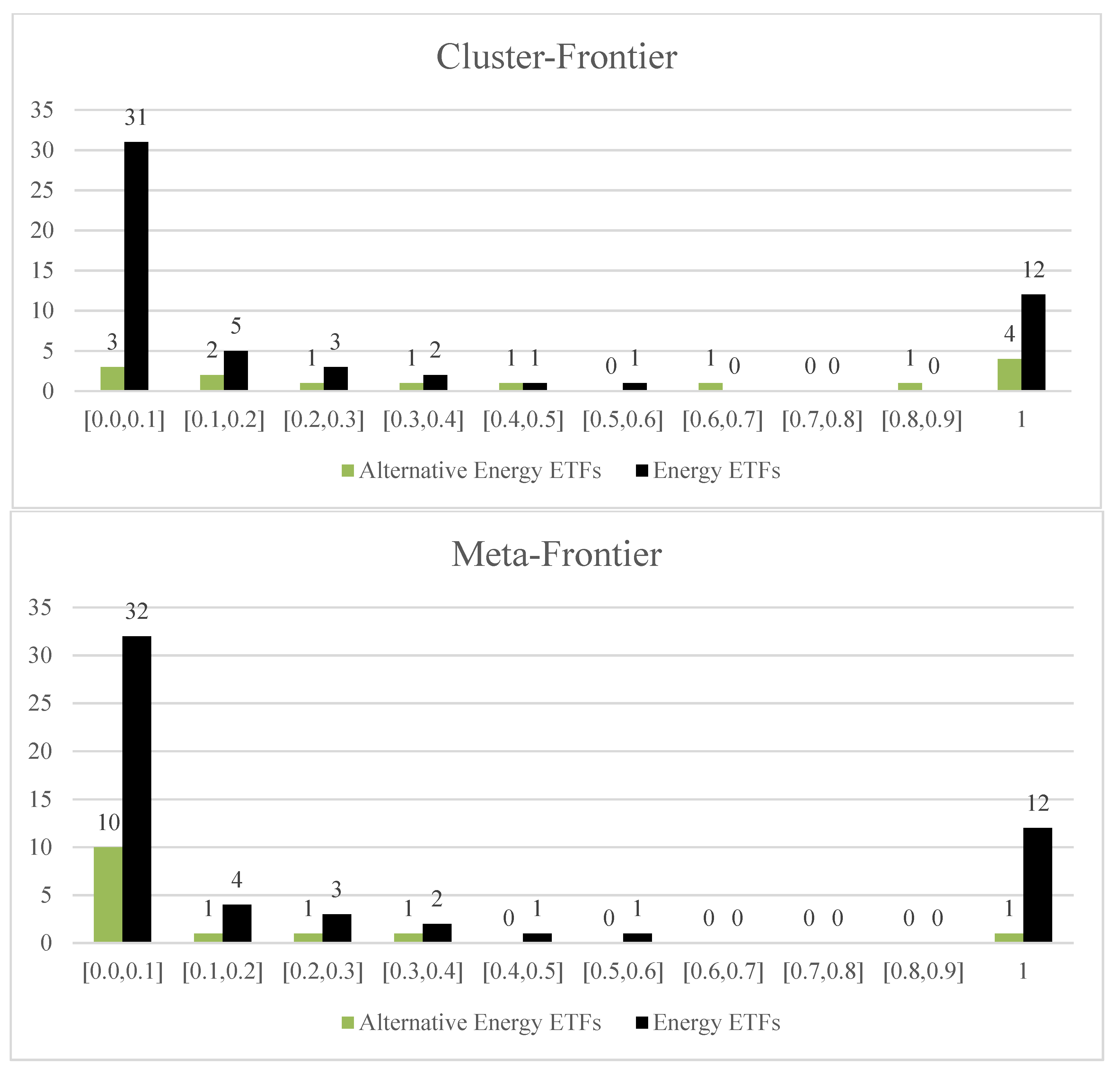
Figure 1 and Figure 2 visually depict the efficiency scores for the meta-frontier and cluster-frontier. The left side showcases the performance of AEEs, while the right side displays the performance of EEs.

The analysis of Figure 3 and Figure 4 reveals a noticeable disparity between the meta-frontier and cluster-frontier for AEEs compared to EEs in both time periods. AEEs exhibit a more significant difference between the two frontiers. This observation is supported by the considerably lower average TGRs for AEEs, with a minimum of 0.26 in the 1-year period, compared to EEs, which have a minimum of 0.96 in the 3-year period. These values indicate a larger gap between the frontiers for AEEs.

Additionally, it is noteworthy that the average TGR values for AEEs slightly decreased over the 3-year period, indicating a growing disparity between the two frontiers, while EEs experienced a slight decrease. This trend suggests that the gap between the meta-frontier and cluster-frontier slightly increased for AEEs, while it slightly narrowed for EEs over the extended time duration.

During the 1-year period, there was a decrease in the number of efficient alternative energy ETFs (AEEs) from the cluster-frontier (4 ETFs) to the meta-frontier (1 ETF), whereas the number of efficient conventional energy ETFs (EEs) remained consistent for both frontiers (12 ETFs)—as depicted in Figure 3.

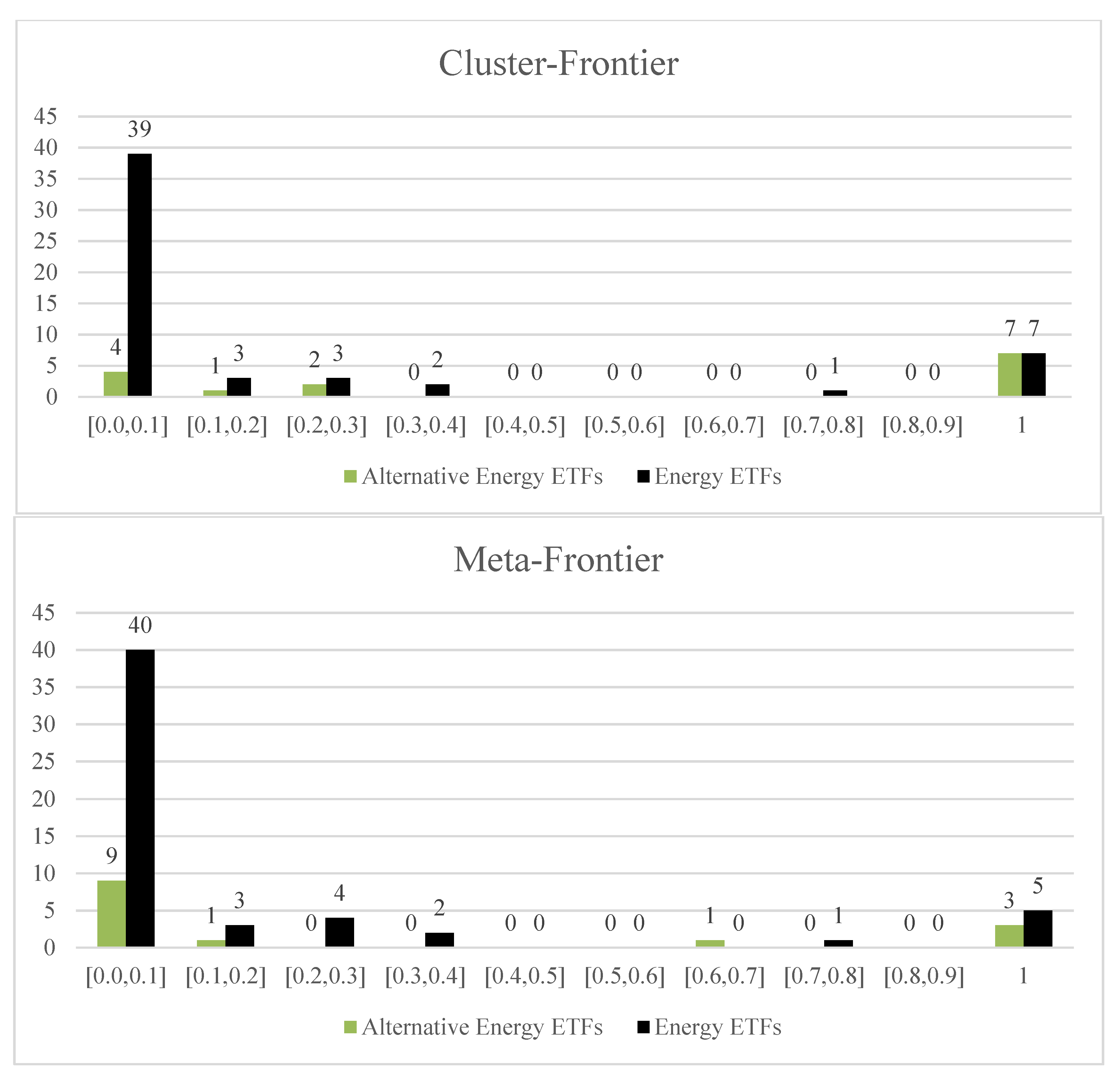
In the 3-year period, there was a decline in the number of efficient AEEs and EEs from the cluster-frontier to the meta-frontier, with a more pronounced decrease observed in the former. Specifically, the number of efficient AEEs decreased from seven to three ETFs. Furthermore, upon conducting a combined analysis of the two periods, it becomes evident that the number of efficient AEEs is higher in the 3-year period, while the number of efficient EEs is higher in the 1-year period—as depicted in Figure 4.

These findings align with the research of Pavlova and Boyrie (2022), who observed that ESG ETFs outperformed the market prior to the crisis but did not exhibit superior performance during the COVID-19 crash. Similarly, Demers et al. (2021) reported that companies with higher ESG scores did not experience superior returns during the COVID-19 crisis. However, contrasting results were reported by Nofsinger and Varma (2014) for the 2000–2011 period, where socially responsible investment (SRI) outperformed conventional funds during the crisis period of 2007–2009.

Table 9. Percentage of efficient ETFs for meta- and cluster-frontiers—1-yr and 3-yr periods.

	Meta-Frontier	Cluster-Frontier
1 yr
Percentage of efficient AEEs	7.14%	28.57%
Percentage of efficient EEs	21.82%	21.82%
3 yrs
Percentage of efficient AEEs	21.43%	50.00%
Percentage of efficient EEs	9.09%	12.73%

presents the percentage of efficient ETFs categorized by type. It is evident that, for the cluster-frontier, the percentage of efficient AEEs surpasses that of efficient EEs in both periods. This indicates that a larger proportion of AEEs are capable of maximizing their outputs.

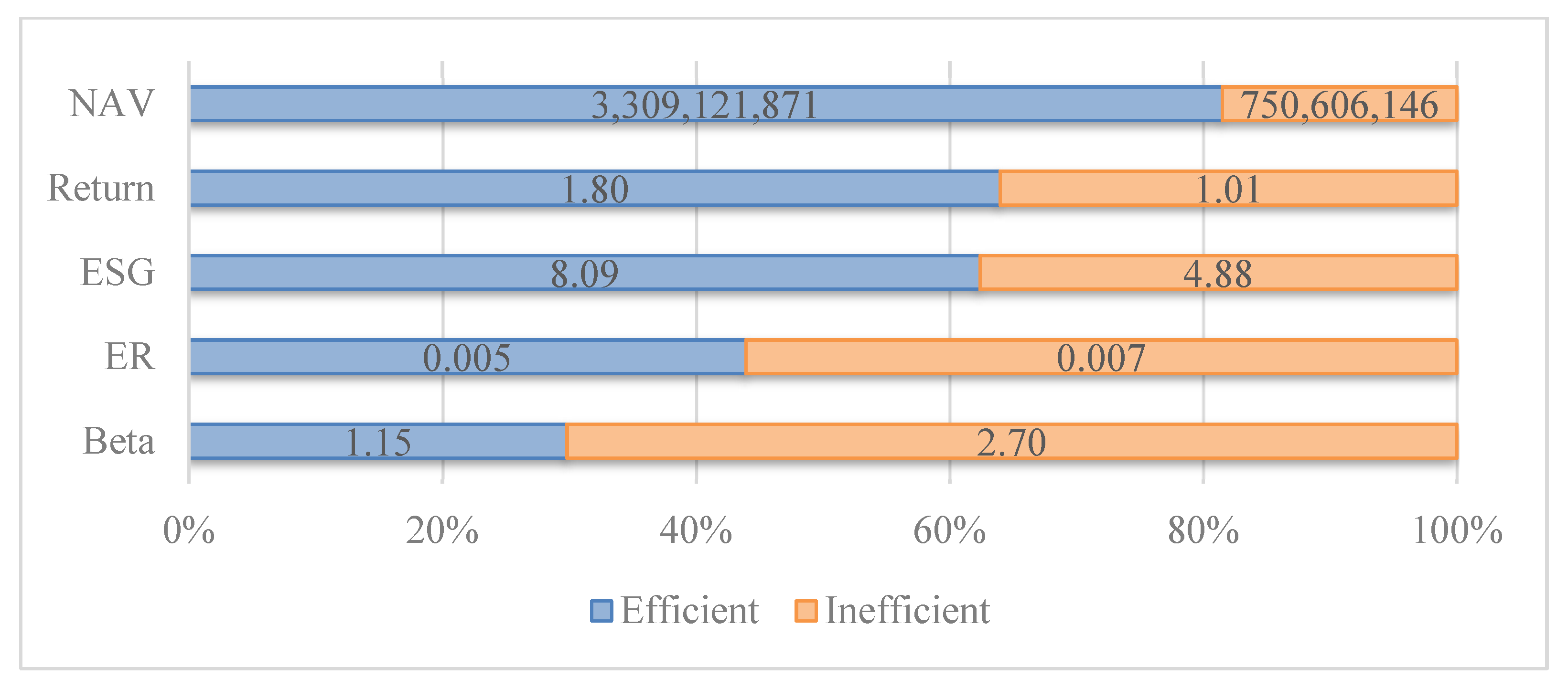
Figure 5 and Figure 6 illustrate that the average values of outputs (NAV, ESG, and return) are significantly higher for efficient ETFs compared to inefficient ones, particularly in the 3-year period. Specifically, efficient funds exhibited higher NAV, ESG, and return values by 341%, 78%, and 66%, respectively. On the other hand, the average values of inputs (beta and ER) are lower for efficient ETFs compared to inefficient ones in both periods, with this difference being more pronounced in the 3-year period. In the 3-year period, efficient funds had lower beta and ER values by 58% and 22%, respectively.

5.1. Potential Improvements

Figure 7 and Figure 8 showcase the potential improvement for each input and output that inefficient ETFs can achieve to become efficient, based on the analysis of the cluster-frontier results. The data presented pertain to a 1-year period and are organized by indicator and ETF category.

Among the indicators, the ER demonstrates the highest potential for improvement, with a remarkable −137%. This implies a reduction in the average ER from 0.0069 to 0.0029. Notably, the potential for improvement in ER is more pronounced for EEs at −182% compared to AEEs at −32%. The NAV also displays a significant improvement potential, averaging 97%. EEs exhibit a higher improvement potential of 97% compared to AEEs at 81%. ESG demonstrates a reasonable average improvement potential of 36%, with a more substantial relevance for EEs at 43% compared to AEEs at 13%. This highlights the importance of environmental, social, and governance factors for EEs compared to AEEs. Return and beta indicate the lowest potential for improvement, with averages of 14% and −5%, respectively. It is noteworthy that the improvement potential for return in AEEs is minimal at 0.4%, while beta shows a more significant value of 10%. Conversely, EEs have a 15% improvement potential for return and a lower value of −4% for beta. Overall, to enhance the efficiency of both EEs and AEEs over the 1-year period, a reduction in the ER and an increase in the NAV are key areas for improvement.

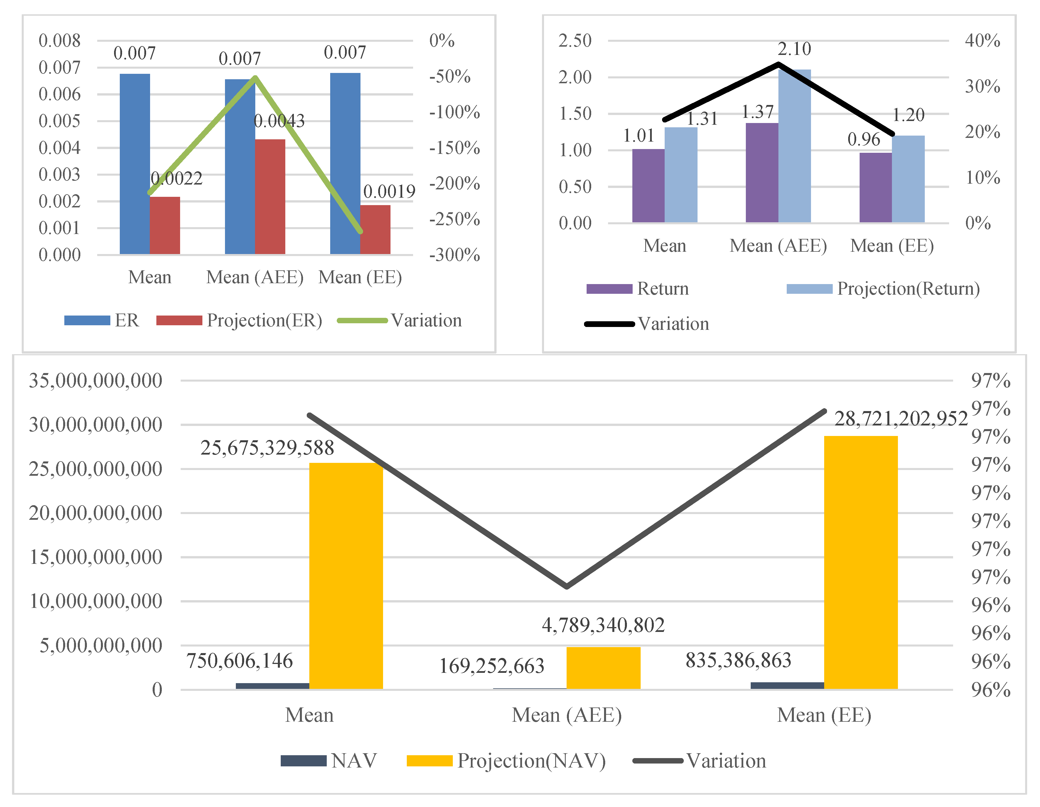
The analysis conducted in the previous section is also applied to a 3-year period, as illustrated in Figure 9 and Figure 10, to examine the impact of time on the results. Similarly to the 1-year period, the ER exhibits the highest potential for improvement, with a remarkable −212%. This indicates a reduction in the average ER from 0.0068 to 0.0022. Consistent with the findings from the 1-year period, the potential for improvement in ER is more pronounced for EEs at −267% compared to AEEs at −52%. The NAV demonstrates the same level of improvement potential as observed in the 1-year period, with nearly identical values for both EEs (97%) and AEEs (96%). ESG values show a similar improvement potential to the 1-year period, with an average of 33%, but with a smaller gap between EEs (37%) and AEEs (17%). Return and beta indicate significantly more room for improvement compared to the 1-year period, with average values of 23% and −22%, respectively. When comparing the 3-year period to the 1-year period, it is noteworthy that AEEs show a higher improvement potential for return (35% versus 20%) while EEs display a 20% improvement potential for return. Therefore, it can be concluded that the average absolute values for improvement potential increase over a longer period (except for ESG). However, the most critical areas for achieving higher efficiency remain the same for both ETF categories—the ER and NAV.

5.2. Correlation Analysis

Table 10. Correlation between the efficiency scores and the input and output factor for each ETF category—1-yr and 3-yr periods.

	1-yr Scores		3-yr Scores
	AEE	EE	AEE	EE
Return	0.199	0.318	0.628	0.271
ER	−0.210	−0.189	−0.423	−0.263
ESG	0.468	0.330	0.285	0.294
Beta	−0.572	0.000	−0.595	−0.398
NAV	0.446	0.310	0.516	0.403

presents the correlation values between the efficiency scores and the indicators for both ETF categories across the two periods. Upon analyzing this table, it becomes evident that there exists a positive correlation between the outputs (return, ESG, and NAV) and the efficiency scores, while a negative (or null) correlation is observed between the inputs (ER and beta) and the efficiency scores. It is also noteworthy that the absolute values of the correlations tend to be stronger over a longer period, with the exception of ESG, which exhibits more relevance over the shorter period, particularly for AEEs. In the 1-year period, the indicator with the strongest correlation to efficiency scores for AEEs is beta (−0.572), while for EEs it is ESG (0.330). Conversely, in the 3-year period, the indicator with the strongest correlation to efficiency scores for AEEs is return (0.628), and for EEs, it is NAV (0.403).

5.3. Robustness Analysis

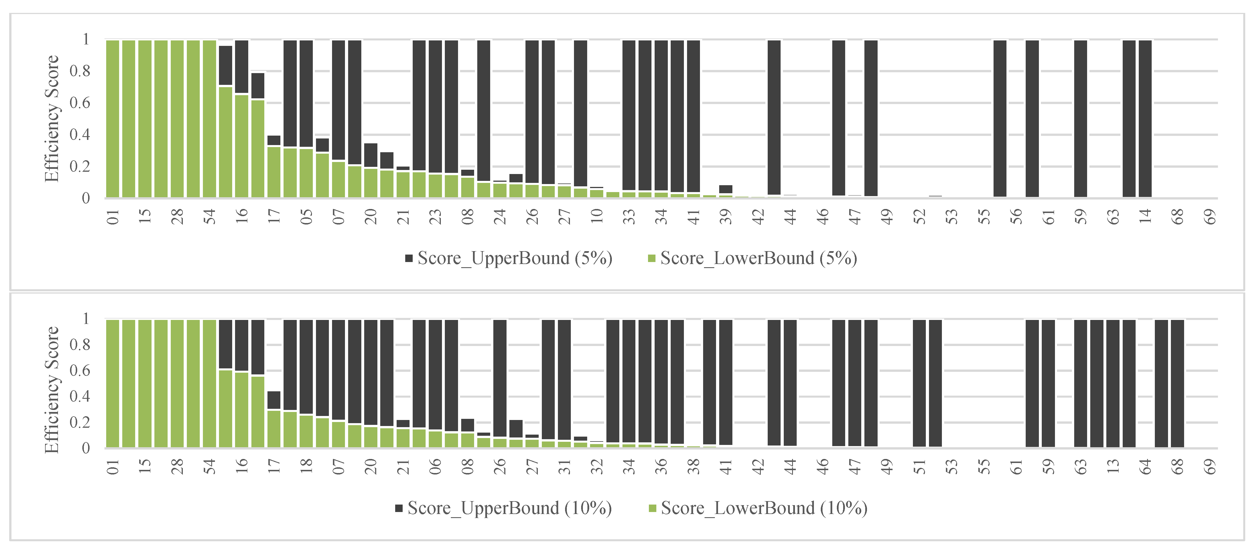
For a 1-year period, when incorporating a tolerance (i.e., a percentage perturbation, representing a deviation in terms of percentage change) of δ = 5% to the current inputs and outputs based on the cluster-frontier, a total of seven ETFs (two AEEs and five EEs) are identified as robustly efficient, while thirty-seven remain robustly inefficient, and twenty-five are potentially efficient. When expanding the tolerance to δ = 10%, the number of robustly efficient ETFs remains the same at seven (two EEs and five AEEs), while twenty-four remain robustly inefficient, and thirty-eight become potentially efficient (see Figure 11). 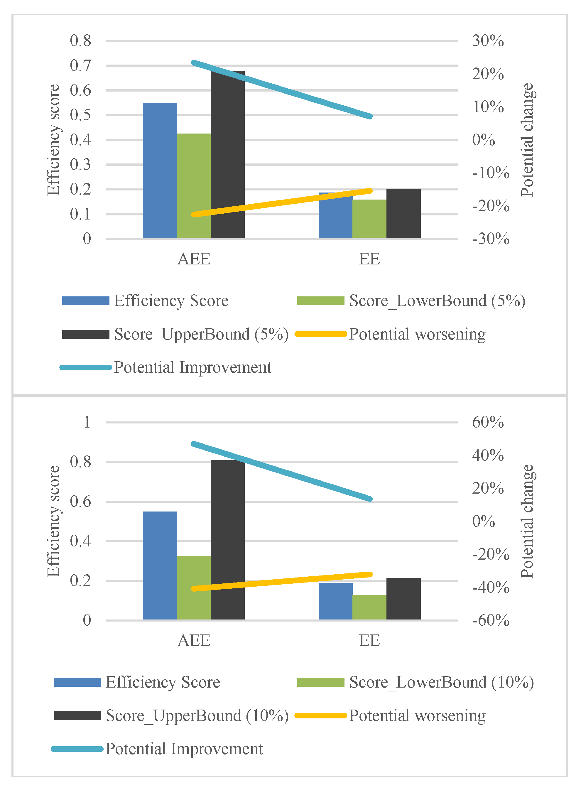Considering a 5% to 10% increase in the factors, AEEs exhibit a potential improvement ranging from 58% to 77%, whereas EEs show a greater potential improvement ranging from 64% to 122% (see Figure 12). Conversely, if all factors experience a 5% to 10% decrease, AEEs are expected to face a potential worsening of −32% to −37%, while EEs show a higher potential worsening ranging from −47% to −50% (see Figure 13). Overall, the efficiency of AEEs demonstrates greater resilience to potential variations in inputs and outputs compared to EEs, which display a more pronounced sensitivity in terms of efficiency.

Over a 3-year period, when considering a tolerance of δ = 5% applied to the inputs and outputs based on the cluster-frontier, eight ETFs (three AEEs and five EEs) are identified as robustly efficient, while fifty-two remain robustly inefficient, and nine are potentially efficient. Expanding the tolerance to δ = 10%, the number of robustly efficient ETFs reduces to six (two EEs and four AEEs), with fifty remaining robustly inefficient and thirteen becoming potentially efficient (refer to Figure 12). Upon increasing the factors by 5% and 10%, AEEs exhibit a potential improvement of 23% to 47%, respectively, whereas EEs show a lower potential improvement ranging from 7% to 14% (see Figure 13). Conversely, when decreasing the factors by 5% and 10%, AEEs experience a potential worsening of −23% to −41%, respectively, while EEs demonstrate a slightly lower potential worsening ranging from −15% to −32% (see Figure 14). In contrast to the observations from the one-year period, EEs demonstrate greater immunity to efficiency variations over the longer term when applying tolerances to the inputs and outputs, compared to AEEs.

Thus, when perturbing inputs and outputs, AEEs exhibit a greater improvement potential than EEs over the longer term, while EEs demonstrate significantly higher room for improvement than AEEs in the short term. Furthermore, it can be observed that the absolute values associated with potential worsening are smaller than those of potential improvement for AEEs in both periods. However, for EEs, the potential worsening becomes more pronounced over the longer term.

6. Conclusions

The rapid growth of the clean energy sector presents an opportunity for investors and fund managers to diversify their portfolios by including firms focused on sustainable energy sources. This study investigates the efficiency of alternative energy ETFs in comparison to conventional energy ETFs, considering both financial and environmental factors. The performance of 14 alternative energy ETFs and 55 conventional energy ETFs was evaluated using an SBM-DEA model over a one-year period (2020) and a three-year period (2018–2020). This non-radial modeling approach provides insights into the necessary adjustments that inefficient ETFs should make to achieve efficiency. By combining the SBM model with cluster analysis, ETFs can be grouped according to their energy type, distinguishing between AEEs and EEs. Furthermore, robustness analysis allows for an assessment of the potential influence on efficiency resulting from changes in factors, which can occur during periods of market turbulence.

When the data are divided into groups based on ETF type, the percentage of efficient AEEs increases significantly, while EEs do not exhibit a strong reaction. TGR values for AEEs are substantially lower, indicating that these ETFs, on average, only achieve 26% and 38% of their potential output over the 1-year and 3-year periods, respectively, when compared to the meta-frontier. Hence, there is a stronger connection between the inputs and outputs used in the assessment for conventional energy ETFs. This outcome could be attributed to the absence of environmental and socially responsible factors, which would likely exhibit a stronger association with alternative energy funds, rather than performance indicators that are more applicable to established and highly valued ETFs.

Introducing 5% and 10% perturbations in the evaluation factors has minimal impact on efficiency, particularly over the longer term, as more than 50 ETFs remain robustly inefficient during this period. However, in the short term, variations in indicators could lead to expanded potential efficiency for more ETFs when increasing the tolerance level. Our results further highlight that the factors that most significantly influence the efficiency of both ETF categories are the ER and NAV. Therefore, reducing operational expenses and improving the assets/liabilities ratio are crucial actions for fund managers to enhance ETF efficiency. Additionally, it is noteworthy that an increase in ESG factors would positively impact conventional energy ETFs to a greater extent than alternative energy ETFs, with even more pronounced effects compared to return or beta.

From an investor’s perspective, it is important to consider how alternative and conventional energy ETFs react to changes in the same indicators, especially during periods of market crises, as investigated in our study. The rapid growth of the clean energy industry and the diversity offered by AEEs present compelling reasons for introducing these securities into investor portfolios. In this study, we have endeavored to provide a set of inputs and outputs that better assess the efficiency of ETF categories from both financial and environmental perspectives. However, we acknowledge that the reported data lack a significant sample of alternative energy ETFs, which could lead to more relevant and comprehensive results.

Future research should incorporate additional indicators to evaluate the efficiency of AEEs and EEs, particularly focusing on more specific indicators based on environmental and socially responsible attributes, alongside substantial data for alternative energy ETFs.

Additional research avenues may explore alternative methodologies, such as investigating the influence of ESG factors on the efficiency of AEEs and EEs through a multi-objective metaheuristic algorithm (e.g., Tian et al. 2023). Alternatively, researchers could delve into the development of an energy-focused stochastic disassembly line balancing problem for AEEs and EEs (e.g., Zhang et al. 2023).