Abstract
This study focuses on efficient asset allocations that properly include T-bills, T-bonds, and the S&P 500 stock index. It checks that their annual real rates of linear return are both normal and almost lognormal. It reexamines how efficient portfolios based on the rates of linear return may turn into efficient portfolios based on the rates of logarithmic return. It finds that each efficient asset allocation has the lowest possible standard deviation as well as the highest possible arithmetic and geometric means. It eventually reconsiders the relationship between the confidence interval of a geometric mean and an expected long-run capital accumulation. As a consequence, it bridges a gap in the scientific literature by enabling financial advisors to trade off the mean rate of return on a portfolio more rigorously against the value at risk.
JEL Classification:
G11; C61; C10
1. Introduction
As recalled by Calverley et al. (2007), there is convincing empirical evidence on variance clustering in many different markets, including equity, currency, and futures markets, especially when sampling is daily or weekly. Variance clustering implies that daily or weekly variance is not constant, so large price changes of either sign tend to follow previous large changes, whereas small price changes of either sign tend to follow previous small changes. A possible cause is that unexpected news tends to come up in clusters. Since the rates of squared or absolute return are serially correlated, variance tends to revert gradually to an appropriate mean value in the short term.
According to Franses and van Dijk (2004), when important stock indices are sampled daily or weekly, their rates of return are not normally distributed. Large negative rates of return are more frequent than large positive rates of return, with outliers being too frequent. Large rates of return tend to occur in clusters that are often triggered by large negative rates of return. As for industrial stocks, the statistical fit of their weekly rates of return is thoroughly examined by Chiang and Li (2015).
However, the annual rates of return have different statistical properties from the daily, weekly, or monthly rates of return. As checked once more by Buzzacchi and Ghezzi (2023), the monthly real rates of linear return on the S&P Composite Index are asymmetric and leptokurtic, whereas the annual real rates of linear return are normal. Indeed, three distinguished chartered financial analysts claim that if asset allocation and investment horizon are appropriate, “the normal distribution may reasonably be used as an approximate model of portfolio returns” (Bronson et al. 2007, p. 54).
This study reconsiders asset allocations that properly include T-bills, T-bonds, and the S&P 500 stock index by using annual real rates of return downloaded by the home page of Professor Aswath Damodaran, New York University in spring 2024. At first, it carries out a preliminary statistical analysis, finding that such efficient asset allocations are normal and stationary in both mean and variance, while also being almost lognormal.
Next, it takes advantage of such statistical properties and explains once more how an efficient frontier based on the annual real rates of linear return turns into a complementary efficient frontier based on the annual real rates of logarithmic return. When it makes use of the above-mentioned annual real rates of return, appropriate efficient asset allocations in a linear space prove efficient in a logarithmic space as well. All efficient asset allocations are lognormal and made up of both stocks and bonds. It also shows that for each given feasible standard deviation, the resulting efficient asset allocation takes the highest possible arithmetic and geometric means.
Finally, it reconsiders the relationship between logarithmic and geometric means. Expanding on Kirkwood (1979), it recalls how to determine an asymmetric confidence interval for an annual geometric mean rate of return. Such a confidence interval comes in useful when calculating an expected long-run capital accumulation.
More generally, rational portfolio management is a systematic process that is composed of three stages, namely planning, executing, and monitoring. Each stage is made up of a few tasks. Feedback and feedforward loops are involved. All stages, tasks, and loops are outlined by Damodaran (2012) and thoroughly presented by Maginn et al. (2007). Selecting asset classes and target weights is the last task in the planning stage. When doing so, both individual and institutional investors may be assisted by financial advisors (Farrell 1997; Maginn et al. 2007). According to business practice, financial advisors should trade off the mean rate of return on a portfolio against the value at risk with an appropriate confidence level (Bronson et al. 2007). This study bridges a gap in the scientific literature by enabling financial advisors to deal with the question more rigorously.
The plan of this study is as follows: the relevant scientific literature is reviewed in Section 2, the dataset is described in Section 3, a preliminary statistical analysis is carried out in Section 4, theoretical and empirical findings are presented in Section 5, and conclusions are drawn in Section 6.
2. Literature Review
Asset allocation concerns the selection of all asset classes and their portfolio weights. It can be stated as a linear-quadratic optimization problem that has a quadratic objective function subject to linear equality and inequality constraints on portfolio weights. The late Dr. Harry Markowitz stated the mean-variance portfolio problem in 1952 (Markowitz and Todd 2000). He devised the critical line algorithm in 1956, which efficiently determines an entire efficient frontier in a finite number of iterations (Markowitz and Todd 2000). He was awarded the 1990 Nobel Prize in Economic Sciences. The milestones of his distinguished career are outlined by Goetzmann (2023).
Mean-variance optimization is performed by Farrell (1997), Sharpe et al. (2007), and Gibson and Sidoni (2013) by diversifying across several asset classes. Mean-variance optimization is also performed by Kumar et al. (2022) by dealing with the stocks listed on the South Pacific Stock Exchange in Fiji.
The use of optimization, simulation, and sensitivity analysis in support of an asset allocation should be complemented with subjective judgment. All relevant procedures rest on the original mean-variance portfolio problem; they were reviewed by Sharpe et al. (2007). Since the original mean-variance portfolio problem deals with the rates of linear return of different asset classes or securities, only arithmetic means are available. Although the arithmetic mean rate of linear return on a portfolio can readily be calculated, it does not lend itself to the determination of an expected capital accumulation.
Let us consider an insightful though peculiar problem of portfolio management by way of an example. Four assumptions are needed: capital is invested only at inception, with coupons and dividends being reinvested; short selling is ruled out; rebalancing occurs once a year to restore the target portfolio weights; and the annual rates of logarithmic return on each portfolio are independent and normally distributed. Since short selling is assumed away, portfolio weights are non-negative. We have
so that each expected long-run accumulation depends on capital, time horizon, and a sample geometric mean. We also have
so that a joint use could be made of the annual rates of logarithmic return, as advocated by Ghezzi (2018).
Therefore, two efficient frontiers can be derived from the four above-mentioned assumptions. As is well known (Markowitz 1991; Rudolf 1994; Sharpe et al. 2007 among others), the efficient frontier based on the annual rates of linear return is continuous, upward-sloping, strictly concave, and piecewise hyperbolic. Each hyperbolic piece is matched by dominant and dominated asset classes; the weights of the former are positive, whereas the weights of the latter are zero. Each hyperbolic piece starts from a corner portfolio and ends in another corner portfolio. In each corner portfolio, a dominant asset class may become dominated or vice versa, or both instances may occur. The asset class with the highest arithmetic mean is a corner portfolio.
As proved by Buzzacchi and Ghezzi (2020), if a sufficient condition is met, all efficient portfolios based on the annual rates of logarithmic return are also efficient portfolios based on the annual rates of linear return, with the opposite being not true. Moreover, the complementary efficient frontier based on the annual rates of logarithmic return is continuous, upward-sloping, and made up of pieces, each having two corner portfolios as bounds. The main outcomes of Ghezzi (2018) and Buzzacchi and Ghezzi (2020) are recapitulated in Appendix A.
Both efficient frontiers are displayed in Section 5 below, where reference is made to three major US asset classes, namely T-bills, T-bonds, and the S&P 500 stock index. Although the same asset classes are also used by Buzzacchi and Ghezzi (2020), historical periods and datasets are different. They check whether the annual rates of logarithmic return on specific portfolios are normally distributed. Such a null hypothesis is rejected for each asset class and some efficient asset allocations, whereas it is not rejected for other efficient asset allocations including all three asset classes.
The aim of this paper is to show that two null hypotheses cannot be rejected. According to the former, the annual rates of linear return on some asset allocations are normally distributed. According to the latter, the annual rates of logarithmic return on the same asset allocations are normally distributed. Let r be an annual rate of linear return and
be the attendant annual rate of logarithmic return. Since the above-mentioned asset allocations include the S&P 500 stock index, T-bonds, and possibly T-bills, Taylor’s expansion truncated at the first order
may be a feasible approximation. Needless to say, whenever both null hypotheses are not rejected, statistical evidence is stronger for the annual rates of linear return.
Both efficient frontiers come in useful when selecting an asset allocation. As documented by Sharpe et al. (2007), asset allocation is the main driving factor of portfolio performance. As proved by Sharpe (1991), if commissions, fees, and personal taxes are assumed away, both market timing and security selection are zero-sum games. As explained by Henriksson and Merton (1981), effective market timing follows from macroforecasting skills, whereas effective security selection follows from microforecasting skills.
Financial advisors may assist both individual and institutional investors (Farrell 1997; Maginn et al. 2007). When selecting an asset allocation along with a client, financial advisors should check that investment objectives are consistent with risk tolerance. According to business practice, they should trade off the mean rate of return on a portfolio against the value at risk (Bronson et al. 2007). As explained in the following, resorting to both efficient frontiers lays a more solid scientific foundation for business practice.
Unfortunately, the means and (co)variances of the annual real rates of linear return are hard to specify, whatever the asset classes (Sexauer and Siegel 2024). According to Black (1993), means are harder to estimate than (co)variances. Moreover, efficient asset allocations are very sensitive to small changes in means and (co)variances and, hence, in estimation errors. As reported by Luenberger (2014) and Sharpe et al. (2007), among others, simulation studies have shown that errors in means have a much larger impact than errors in (co)variances. Owing to possible estimation errors, efficient asset allocations may have extreme weights so that important asset classes may be unrepresented. As explained by Gibson and Sidoni (2013), a heuristic remedy is to place lower and upper bounds on the weights of all asset classes so that a considerable part of an asset allocation is decided in advance. Although the resulting efficient asset allocations are suboptimal, they benefit from broad diversification because they include all asset classes. The imposition of additional constraints on stock portfolios is investigated in the pioneering work by Frost and Savarino (1988). Abate et al. (2022) reviewed the relevant literature and extended the analysis to the constrained diversification across the sectors of the MSCI All Country World Index.
3. Dataset
Data were downloaded in the spring of 2024 from the home page of Professor Aswath Damodaran, New York University. Data cover the historical period 1928–2023 and take the form of annual rates of return, both nominal and real. Three major US asset classes were selected: 3-month T-bills, 10-year T-bonds, and the S&P 500 stock index.
As explained by Professor Damodaran, the rates of return on the S&P 500 take dividends into account, the rates of return on 3-month T-bills are annual averages, and the yields to maturity on 10-year US T-bonds are provided by FRED, the database run by the Federal Reserve Bank of St. Louis. Professor Damodaran had turned yields to maturity into rates of return under the convenient assumption that 10-year T-bonds are issued at par. In total, 96 annual real rates of linear return as well as 96 annual real rates of logarithmic return were downloaded for each asset class along with 96 annual rates of inflation.
The sample statistics are reported in Table 1 for linear rates and in Table 2 for logarithmic rates.

Table 1.
Statistics of three asset classes. Annual real rates of linear return, 1928–2023.
Table 2.
Statistics of three asset classes. Annual real rates of logarithmic return, 1928–2023.
Linear and logarithmic rates display the same percentage of negative rates by definition; such percentages are higher for T-bills and T-bonds, in spite of narrower ranges. As expected, the annual real rates of linear return on the S&P 500 have a very modest asymmetry and kurtosis excess. This is a clue that they are normally distributed.
The logarithmic rates on T-bills and the S&P 500 stock index tend to display more asymmetry and kurtosis excess than linear rates. In contrast, the logarithmic rates on T-bonds tend to display less asymmetry than linear rates, with kurtosis excess remaining unchanged.
The correlation matrix is reported in Table 3 for both linear and logarithmic rates, which display very similar cross-correlations. The S&P 500 stock index is poorly correlated with both T-bills and T-bonds.
Table 3.
Correlation matrices of three asset classes. (a) Real rates of linear return, 1928–2023. (b) Real rates of logarithmic return, 1928–2023.
4. Preliminary Statistical Analysis
4.1. Normality and Lognormality Tests
The null hypothesis of normally distributed rates of return is investigated by having recourse to Anderson–Darling, Jarque–Bera, Lilliefors, and Shapiro–Wilk tests: when a p-value exceeds the 0.05 threshold, the null hypothesis is not rejected. The p-values for all asset classes are reported in Table 4. The annual real rates on the S&P 500 stock index are normally distributed according to all four tests, whereas the annual real rates on T-bills are not and have the highest confidence level. Both occurrences are known. Remarkably, the annual real rates on T-bonds are normally distributed as well.
Table 4.
Normality tests: p-values for the asset classes.
The p-values for three asset allocations are reported in Table 5. All asset allocations lie on the efficient frontier; they are determined by applying the critical line algorithm to available data. Additional information on the efficient frontier is provided in Section 5.
Table 5.
Normality tests: p-values for three asset allocations. , , and are the weights of T-bills, T-bonds, and the S&P 500, respectively.
The first asset allocation includes all three asset classes, whereas the other two asset allocations include only T-bonds and the S&P 500. Remarkably, the annual real rates on all asset allocations are normally distributed according to all four tests, which agrees with the above-mentioned claim of Bronson et al. (2007).
The null hypothesis of lognormally distributed rates of return is investigated by having recourse to Anderson–Darling, Jarque–Bera, Lilliefors, and Shapiro–Wilk tests: when a p-value exceeds the 0.05 threshold, the null hypothesis is not rejected. The p-values for all asset classes are reported in Table 6. Only the annual real rates on T-bonds are lognormally distributed. Therefore, approximation (4) does not work well for the S&P 500 stock index.
Table 6.
Lognormality tests: p-values for the asset classes.
The p-values for the three above-mentioned efficient asset allocations are reported in Table 7. Evidence is mixed: according to Anderson–Darling, Jarque–Bera, and Lilliefors tests, the annual real rates on all asset allocations are lognormally distributed; according to the Shapiro–Wilk test no asset class is lognormal. Since all p-values of the Shapiro–Wilk test are not far from 0.05, approximation (4) seems to work fairly well for all asset allocations.
Table 7.
Lognormality tests: p-values for three asset allocations. , , and are the weights of T-bills, T-bonds, and the S&P 500, respectively.
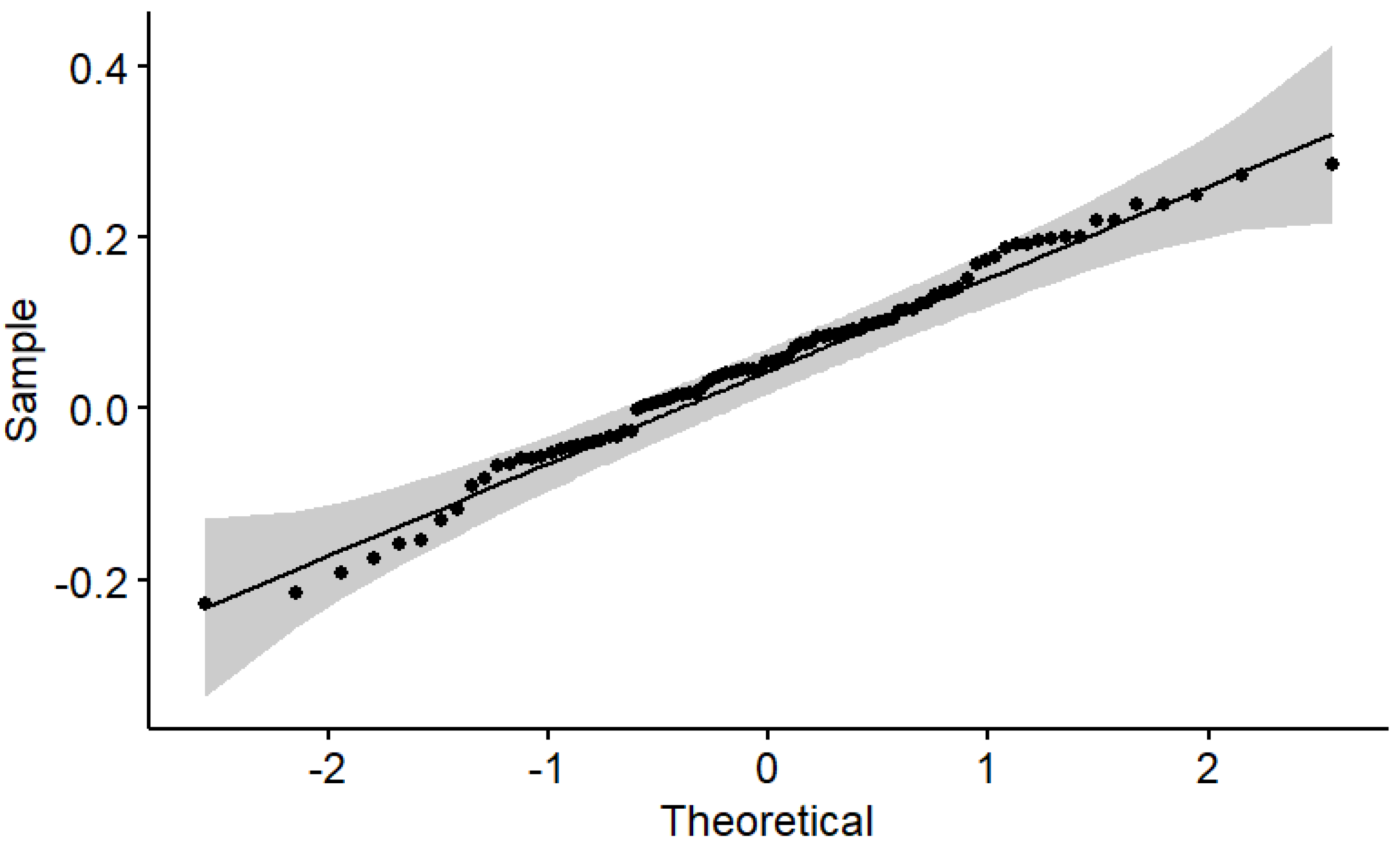
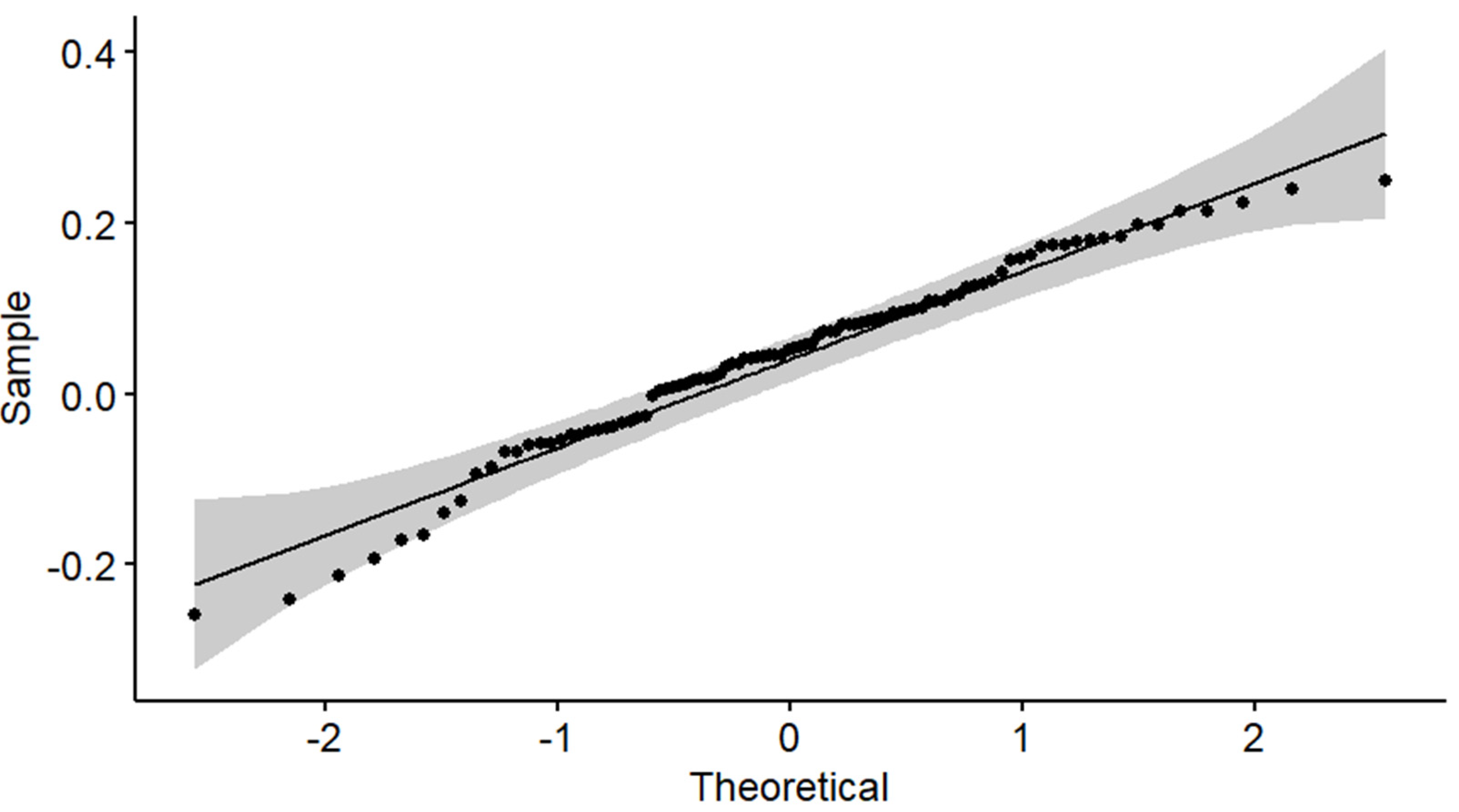
Quantile–quantile plots are constructed in order to further investigate both hypotheses. For instance, the empirical distribution of the annual real rates of linear return on the intermediate asset allocation is compared with a normal distribution in Figure 1, whereas the empirical distribution of the annual real rates of logarithmic return on the intermediate asset allocation is compared with a normal distribution in Figure 2. The confidence level of the shaded area is 0.95. Indeed, the intermediate asset allocation of 50% T-bonds and 50% S&P 500 stock index seems to be both normal and almost lognormal. The quantile–quantile plots for the other two asset allocations are qualitatively similar.
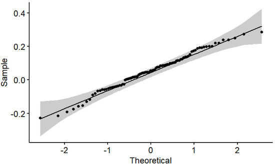
Figure 1.
Annual real rates of linear return on the intermediate asset allocation. Quantile–quantile plot.
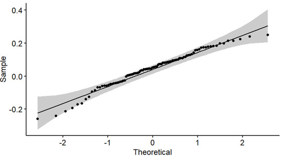
Figure 2.
Annual real rates of logarithmic return on the intermediate asset allocation. Quantile–quantile plot.
Altogether, the null hypothesis of normality is rejected for one asset class, whereas the null hypothesis of lognormality is rejected for two asset classes. In contrast, all three asset allocations are normally distributed, also being almost lognormally distributed. The resulting empirical evidence is in accordance with Buzzacchi and Ghezzi (2020). The power of normality tests is a challenging problem, which is tackled by Yazici and Yolacan (2007) and Noughabi and Arghami (2011), among others. The sample size in this study is 96; it is neither small nor large, being moderate. The outcomes of all four normality tests are always in agreement, with all quantile–quantile plots being consistent. Moreover, there also seems to be agreement with the asymmetries and kurtosis excesses of all asset classes.
Since efficient asset allocations including both stocks and bonds benefit from aggregational normality, the use of mean and variance as decision criteria proves correct, a possibility originally pointed out by Tobin (1958). Remarkably, the legendary value investor Benjamin Graham claimed that the standard asset allocation of a defensive investor should be 50% stocks and 50% bonds (Graham et al. 2006).
4.2. Unit Root Tests
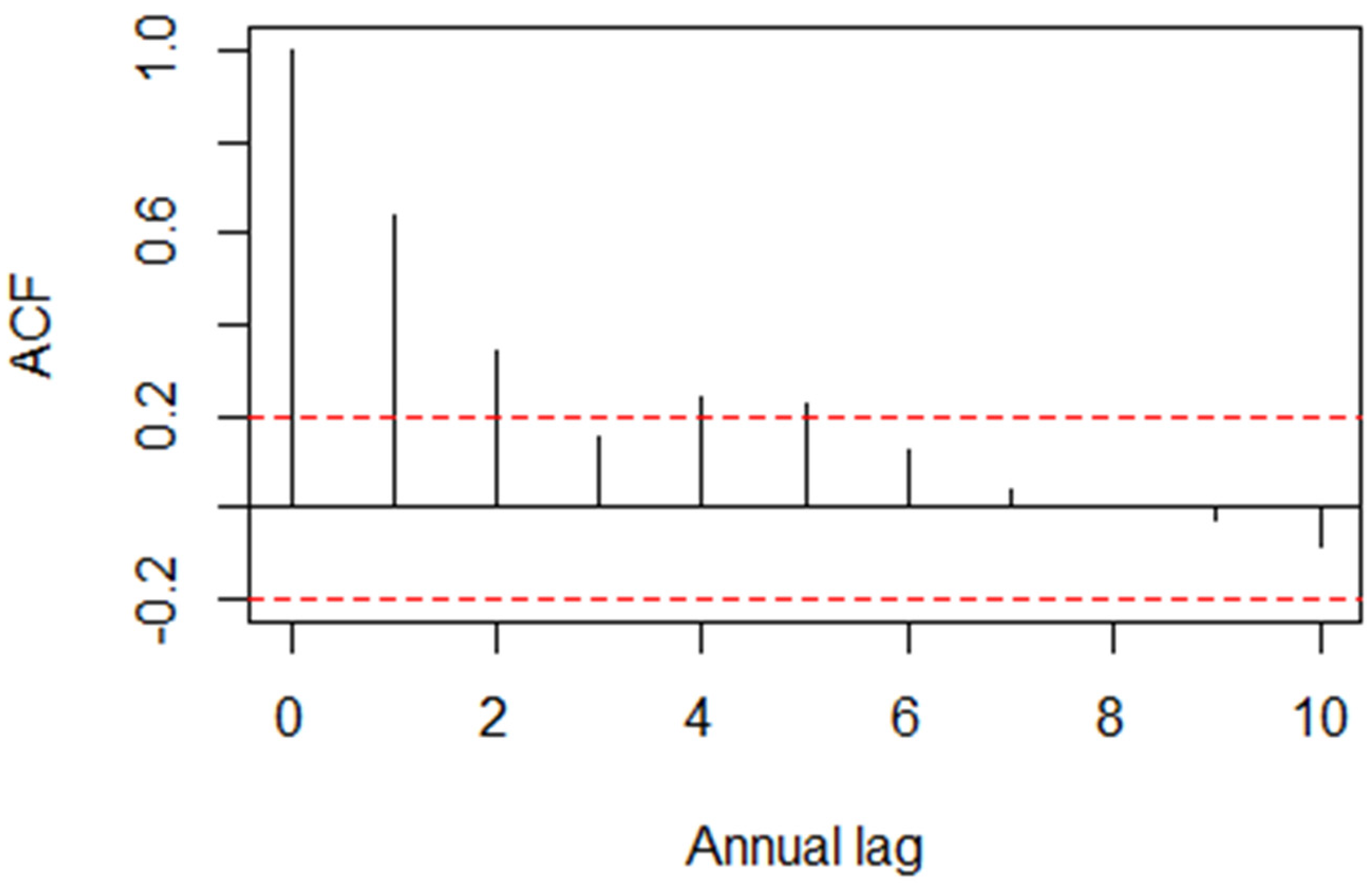
The autocorrelation function for the annual real rates of linear return on T-bills is displayed in Figure 3. Indeed, the one- and two-year sample autocorrelations lie outside the 0.95 confidence interval. As for the other two asset classes, all sample autocorrelations lie inside the 0.95 confidence interval.
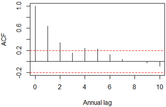
Figure 3.
Annual real rates of linear return on T-bills. Autocorrelation function.
All three autocorrelation functions for the annual real rates of logarithmic return are not reported. They are qualitatively similar to the autocorrelation functions for the annual real rates of linear return.
Unit root tests are performed on all asset classes and efficient asset allocations. In each instance, a null hypothesis of random walk is tested by carrying out unit root tests on 96 annual real rates of logarithmic return. The relevant literature on unit root tests is summarized by Nguyen et al. (2022). Let time be measured in years and be the market value of a portfolio at the end of year t. Suppose that the market value takes a discrete-time random walk
where the error term is an annual real rate of logarithmic return that is part of a sequence of independent and identically distributed random variables. We assume away the occurrence of structural breaks.
According to both augmented Dickey–Fuller and Phillips–Perron tests, the null hypothesis of a unit root is rejected for all asset classes, with the significance level being 0.01 for the S&P 500 stock index and 0.05 for T-bills and T-bonds. Therefore, all asset classes seem to be trend-stationary rather than difference-stationary. This is preliminary empirical evidence since the possible occurrence of structural breaks is not examined.
Surprisingly, the evidence on the three efficient asset allocations in Table 5 is mixed. The null hypothesis of a unit root is rejected for the first two asset allocations, whereas it is accepted for the third asset allocation. The significance level is always 0.05.
4.3. Basic Stationarity Tests
Additional stationarity tests are performed by splitting the historical period of 1928–2023 into two subperiods of 1928–1972 and 1973–2023, consisting of 45 and 51 years, respectively. Reference is made to two asset classes, T-bonds and the S&P 500 stock index, and all efficient asset allocations since their annual real rates of linear return are normally distributed.
Let be an arithmetic mean rate of return and be the attendant standard deviation; both statistics belong either to the former or latter subperiod. According to the first null hypothesis, the two sample means and come from populations that have the same mean. According to the second null hypothesis, the two sample variances and come from populations that have the same variance. The p-values for all asset classes are reported in Table 8. T-bonds are stationary in mean, whereas the S&P 500 stock index is stationary in both mean and variance.
Table 8.
Stationarity tests: p-values for two asset classes.
The p-values for all efficient asset allocations are reported in Table 9. Remarkably, all asset allocations are stationary in both mean and variance.
Table 9.
Stationarity tests: p-values for three asset allocations. , , and are the weights of T-bills, T-bonds, and the S&P 500, respectively.
The sample means and variances in Table 9 can be compared with some of the sample means and variances in Table 10 below, which concerns the whole historical period. According to our basic stationarity tests, 45–50 years of annual data seem to be an appropriate sample size when it comes to estimating means and (co)variances from historical data. As advocated by Bernstein (1997), each sample should start and end with similar multiples, for instance, similar price–earnings ratios.
Table 10.
Efficient asset allocations: mean rate of linear return and standard deviation. , , and are the weights of T-bills, T-bonds, and the S&P 500, respectively.
5. Theoretical and Empirical Findings
5.1. Efficient Asset Allocations
We let time be measured in years and capital be invested only at inception, with coupons and dividends being reinvested and rebalancing occurring once a year to restore the target portfolio weights. We rule out short selling and assume away commissions, fees, and personal taxes. We also assume that the annual real rates of return on each asset allocation are independent and identically distributed, with population moments being the same as past sample moments.
At first, we consider the efficient asset allocations based on the annual real rates of linear return. Let be an arithmetic mean rate of return and be the attendant standard deviation. Applying the critical line algorithm to available data obtains an efficient frontier that lies in the linear space . The code in Visual Basic for Applications is presented by Markowitz and Todd (2000). Some efficient asset allocations based on the annual real rates of linear return are reported in Table 10.
The efficient frontier includes four corner portfolios: the minimum-variance portfolio P, which excludes T-bonds, portfolios A and B, as well as the maximum-variance portfolio C, which is the S&P 500 stock index. The minimum-variance portfolio P and the tangent portfolio T are very close to each other; the role played by the latter is explained below. Table 10 also includes the efficient asset allocations examined in Table 5, Table 7, and Table 9. Since their arithmetic means and standard deviations take intermediate values, normality and almost lognormality seem to follow from appropriate risk mitigation.
The computation of value at risk is straightforward because the annual real rates of linear return are normal. The advantages and limitations of value at risk are examined by Chance et al. (2007) and Resti and Sironi (2007). As advocated by Bronson et al. (2007), value at risk should depend on the worst possible annual real rate with a 97.72% confidence level, namely
Next, we consider the efficient asset allocations based on the annual real rates of logarithmic return. Let be a logarithmic mean rate of return and be the attendant standard deviation. Although only the annual real rates of linear return on some intermediate asset allocations are almost lognormally distributed, an entire complementary efficient frontier is derived for the sake of clarity. More precisely, the moments map onto the moments in accordance with the following equations (Crow and Shimizu 1988):
As recapitulated in Appendix A, if a sufficient condition is met, applying Equations (7) and (8) to the efficient frontier that lies in the linear space results in a complementary efficient frontier that lies in the logarithmic space . Accordingly, Table 10 above turns into Table 11 below.
Table 11.
Efficient asset allocations: mean rate of logarithmic return and standard deviation. , , and are the weights of T-bills, T-bonds, and the S&P 500, respectively.
The complementary efficient frontier includes four corner portfolios: the minimum-variance portfolio T, portfolios A and B, as well as the maximum-variance portfolio C, which is the S&P 500 stock index. Since portfolio P is now inefficient, the tangent portfolio T becomes the minimum-variance portfolio. Accordingly, Table 10 and Table 11 share three corner portfolios. The means and variance in Table 11 display narrower ranges and lower upper bounds than the means and variance in Table 10.
5.2. Geometric Means
Since the minimum-variance portfolio P and the tangent portfolio T are very close to each other, efficiency in the linear space is approximately the same as efficiency in the logarithmic space . As previously assumed in Section 5.1, the elements of both spaces are pairs of population moments.
Therefore, each efficient asset allocation lies on two different efficient frontiers and has the highest possible arithmetic mean given the attendant standard deviation as well as the highest possible logarithmic mean given the attendant standard deviation . Since both efficient frontiers slope upward, the highest possible arithmetic mean goes along with the highest possible logarithmic mean and, hence, with the highest possible geometric mean owing to Equation (2).
Although the sample geometric mean on a portfolio is unknown until the time horizon is reached, a narrower confidence interval goes along with a more distant time horizon. Such a confidence interval can be readily obtained by expanding on Kirkwood (1979). We set the significance level to 4.55% and let n be the sample size. The confidence interval is asymmetric and equal to
In principle, Equation (9) applies only to intermediate asset allocations including both stocks and bonds since they are almost lognormally distributed. Both an expected long-run accumulation and an annual value at risk should be taken into account when selecting an appropriate efficient asset allocation. In this setting, the former is given by Equation (1), whereas the latter follows from Equation (6).
The investment goals of an individual investor may be a college education for children, a second home, or a serene retirement. Investment goals are eventually turned into an investment objective, e.g., a desired capital accumulation at a set and distant time horizon. When selecting an asset allocation along with a client, financial advisors should check that investment objectives are consistent with risk tolerance. According to business practice, financial advisors should trade off the mean rate of return on a portfolio against the annual value at risk (Bronson et al. 2007).
In the setting of this study, meeting the investment objective depends on Equation (1), whereby each expected long-run accumulation depends on capital, time horizon, and a geometric mean rate of return. Equation (1) is in line with the remark made by MacBeth (1995). Complying with an individual risk tolerance depends on Equation (6), which calculates the annual value at risk with a 97.72% confidence level. This is the procedure outlined by Bronson et al. (2007). Therefore, resorting to both efficient frontiers conveys more rigor in business practice.
6. Conclusions
An efficient frontier is determined in this study by applying the critical line algorithm to almost a century of data on T-bills, T-bonds, and the S&P 500 stock index. The annual real rates of linear return on some intermediate efficient asset allocations are shown to be stationary in mean and variance and to benefit from aggregational normality, while also being almost lognormal. However, the possible occurrence of structural breaks is not examined.
Each intermediate efficient asset allocation includes an appropriate mix of stocks and bonds. The latter plays a twofold role: as remarked by Graham et al. (2006) and Gibson and Sidoni (2013), among others, bonds mitigate risk; moreover, since they reduce the range of possible outcomes, they also make the normal efficient asset allocations almost lognormal.
Upon assuming that the annual real rates of logarithmic return are independent and normally distributed, a complementary efficient frontier is also determined. Since some efficient asset allocations are almost lognormal, each given feasible standard deviation is matched by the highest possible arithmetic and geometric means. An asymmetric confidence interval for an annual geometric mean rate of return is eventually derived so that an expected long-run capital accumulation can be calculated more accurately.
According to business practice, financial advisors should trade off the annual mean rate of return on a portfolio against the annual value at risk with a 97.72% confidence level. This study bridges a gap in the scientific literature by enabling financial advisors to deal with the question more rigorously. When trading off reward against risk, financial advisors should make use of the above-mentioned annual geometric mean rate of return. Since emphasis is placed on the very long run, reference is made to a strategic asset allocation rather than to a tactical one.
The present treatment has two main limitations. On the one hand, it does not fix the main drawback of the mean-variance approach: the means and (co)variances of the annual rates of linear return are hard to specify. On the other hand, it deals with long-only asset allocations without admitting the statement of additional inequality constraints.
Funding
No research grant has been received in support of this scientific work.
Informed Consent Statement
Not applicable.
Data Availability Statement
Data downloaded from https://pages.stern.nyu.edu/~adamodar/ accessed on 9 April 2024.
Acknowledgments
The author is grateful to Elena Conti for her editorial support and to Riccardo Micheloni for his bibliographical assistance. He also thanks his colleague Luigi Buzzacchi (Politecnico di Torino) and two anonymous reviewers for their useful comments and suggestions. As usual, he is solely responsible for any remaining errors.
Conflicts of Interest
The author declares no conflicts of interest.
Appendix A
Let time be measured in years, be the arithmetic mean rate of return on an asset allocation, and be the attendant standard deviation. If long-short asset allocations are allowed, the efficient frontier is a hyperbola that takes the form (Merton 1972)
where the four real parameters (Rudolf 1994)
can be estimated from available data by using the unit vector , the mean vector , and the variance-covariance matrix , which should be real, symmetric, and positive definite. We also have (Rudolf 1994)
where the vector contains the weights of an efficient asset allocation that meets Equation (A1).
Assume that the annual rates of logarithmic return on each asset allocation are independent and normally distributed. Let be a logarithmic mean rate of return and be the attendant standard deviation. The discriminant
is eventually obtained by taking advantage of the one-to-one mapping (7) and (8). Consider the tangent portfolio T that lies above the minimum-variance portfolio P in the linear space and maps onto the minimum-variance portfolio T in the logarithmic space . Such a portfolio can be determined by setting the risk-free rate to −1 and applying the one-fund theorem, which is restated in Luenberger (2014).
As proved by Ghezzi (2018), all efficient or minimum-variance asset allocations below point T in the linear space turn into minimum-variance asset allocations in the logarithmic space. Moreover, all efficient asset allocations above point T in the linear space turn into efficient asset allocations in the logarithmic space for , whereas some efficient asset allocations above point T turn into inefficient asset allocations for . If the means and (co)variances are retrieved from Table 1 and Table 3, the parameters (A2) take the values so that . We have and for portfolio P as well as and for portfolio T; therefore, the minimum-variance portfolio P and the tangent portfolio T are very close to each other. Both portfolios have a short position in T-bonds.
If long-only asset allocations are considered, the efficient frontier based on the annual rates of linear return is continuous, upward-sloping, strictly concave, and piecewise hyperbolic. Let the tangent portfolio T lie above the minimum-variance portfolio P in the linear space and map into the minimum-variance portfolio T in the logarithmic space . Portfolios P and T are reported in Table 10; both portfolios exclude T-bonds. According to the sufficient condition proved by Buzzacchi and Ghezzi (2020), all efficient asset allocations between point P and point T in the linear space turn into minimum-variance asset allocations in the logarithmic space. Moreover, all efficient asset allocations above point T in the linear space turn into efficient asset allocations in the logarithmic space under the assumption that each hyperbolic piece of the efficient frontier based on the annual rates of linear return is matched by either or with the attendant hyperbola attaining a local maximum beyond the corner portfolio on the right.
The efficient frontier based on the annual rates of logarithmic return is a piecewise continuous and upward-sloping function; it starts from a corner portfolio with global minimum variance and ends in a corner portfolio with global maximum variance. The concavity of such an efficient frontier has not been studied yet.
References
- Abate, Guido, Tommaso Bonafini, and Pierpaolo Ferrari. 2022. Portfolio constraints: An empirical analysis. International Journal of Financial Studies 10: 9. [Google Scholar] [CrossRef]
- Bernstein, Peter L. 1997. What rate of return can you reasonably expect … or what can the long run tell us about the short run? Financial Analysts Journal 53: 20–28. [Google Scholar] [CrossRef]
- Black, Fischer. 1993. Estimating expected return. Financial Analysts Journal 49: 36–38. [Google Scholar] [CrossRef]
- Bronson, James W., Matthew H. Scanlan, and Jan R. Squires. 2007. Managing individual investor portfolios. In Managing Investment Portfolios. A Dynamic Process, 3rd ed. Edited by John L. Maginn, Donald L. Tuttle, Dennis W. McLeavey and Jerald E. Pinto. Hoboken: Wiley, pp. 20–58. [Google Scholar]
- Buzzacchi, Luigi, and Luca Ghezzi. 2020. Asset allocation with nonnegative weights and lognormal portfolio returns. International Review of Business Research Papers 16: 1–15. [Google Scholar]
- Buzzacchi, Luigi, and Luca Ghezzi. 2023. Mean reversion lessens mean blur: Evidence from the S&P composite index. International Journal of Financial Studies 11: 1–13. [Google Scholar]
- Calverley, John P., Alan M. Meder, Brian D. Singer, and Renato Staub. 2007. Capital market expectations. In Managing Investment Portfolios. A Dynamic Process, 3rd ed. Edited by John L. Maginn, Donald L. Tuttle, Dennis W. McLeavey and Jerald E. Pinto. Hoboken: Wiley, pp. 128–229. [Google Scholar]
- Chance, Don M., Kenneth Grant, and John Marsland. 2007. Risk management. In Managing Investment Portfolios. A Dynamic Process, 3rd ed. Edited by John L. Maginn, Donald L. Tuttle, Dennis W. McLeavey and Jerald E. Pinto. Hoboken: Wiley, pp. 579–636. [Google Scholar]
- Chiang, Thomas C., and Jiandong Li. 2015. Modeling asset returns with skewness, kurtosis, and outliers. In Handbook of Financial Econometrics and Statistics. Edited by Cheng-Few Lee and John C. Lee. New York: Springer, pp. 2177–215. [Google Scholar]
- Crow, Edwin L., and Kunio Shimizu, eds. 1988. Lognormal Distributions: Theory and Applications. New York: Marcel Dekker Inc. [Google Scholar]
- Damodaran, Aswath. 2012. Investment Philosophies, 2nd ed. Hoboken: Wiley. [Google Scholar]
- Farrell, James L. 1997. Portfolio Management: Theory and Application, 2nd ed. New York: Irwin McGraw-Hill. [Google Scholar]
- Franses, Philip H., and Dick van Dijk. 2004. Non-Linear Time Series Models in Empirical Finance. Cambridge: Cambridge University Press. [Google Scholar]
- Frost, Peter A., and James E. Savarino. 1988. For better performance: Constrain portfolio weights. Journal of Portfolio Management 15: 29–34. [Google Scholar] [CrossRef]
- Ghezzi, Luca. 2018. Asset allocation under lognormal portfolio returns. International Review of Business Research Papers 14: 146–63. [Google Scholar] [CrossRef]
- Gibson, Roger C., and Christopher J. Sidoni. 2013. Asset Allocation. Balancing Financial Risk, 5th ed. New York: McGraw-Hill. [Google Scholar]
- Goetzmann, William N. 2023. Harry Markowitz in memoriam. Financial Analysts Journal 79: 5–7. [Google Scholar] [CrossRef]
- Graham, Benjamin, Jason Zweig, and Warren E. Buffett. 2006. The Intelligent Investor. A Book of Practical Counsel, rev. ed. New York: Harper. [Google Scholar]
- Henriksson, Roy. D., and Robert C. Merton. 1981. On market timing and investment performance. II. Statistical procedures for evaluating forecasting skills. Journal of Business 54: 513–33. [Google Scholar] [CrossRef]
- Kirkwood, Thomas B. L. 1979. Geometric means and measures of dispersion. Biometrics 35: 908–9. [Google Scholar]
- Kumar, Ronald R., Peter J. Stauvermann, and Aristeidis Samitas. 2022. An application of portfolio mean-variance and semi-variance optimization techniques: A case of Fiji. Journal of Risk and Financial Management 15: 190. [Google Scholar] [CrossRef]
- Luenberger, David G. 2014. Investment Science, 2nd ed. New York: Oxford University Press. [Google Scholar]
- MacBeth, James D. 1995. What’s the long-term expected return to your portfolio? Financial Analysts Journal 51: 6–8. [Google Scholar] [CrossRef]
- Maginn, John L., Donald L. Tuttle, Dennis W. McLeavey, and Jerald E. Pinto. 2007. The portfolio management process and the investment policy statement. In Managing Investment Portfolios. A Dynamic Process, 3rd ed. Edited by John L. Maginn, Donald L. Tuttle, Dennis W. McLeavey and Jerald E. Pinto. Hoboken: Wiley, pp. 1–19. [Google Scholar]
- Markowitz, Harry M. 1991. Portfolio Selection. Efficient Diversification of Investments, 2nd ed. Cambridge: Basil Blackwell. [Google Scholar]
- Markowitz, Harry M., and G. Peter Todd. 2000. Mean-Variance Analysis in Portfolio Choice and Capital Markets. New York: Wiley. [Google Scholar]
- Merton, Robert C. 1972. An analytic derivation of the efficient portfolio frontier. Journal of Financial and Quantitative Analysis 7: 1851–72. [Google Scholar] [CrossRef]
- Nguyen, James, Wei-Xuan Li, and Clara Chia-Sheng Chen. 2022. Mean Reversions in Major Developed Stock Markets: Recent Evidence from Unit Root, Spectral and Abnormal Return Studies. Journal of Risk and Financial Management 15: 162. [Google Scholar] [CrossRef]
- Noughabi, Hadi A., and Naser R. Arghami. 2011. Monte Carlo comparison of seven normality tests. Journal of Statistical Computation and Simulation 81: 965–72. [Google Scholar] [CrossRef]
- Resti, Andrea, and Andrea Sironi. 2007. Risk Management and Shareholders’ Value in Banking. Chichester: Wiley. [Google Scholar]
- Rudolf, Markus. 1994. Algorithms for Portfolio Optimization and Portfolio Insurance. Bern: Haupt. [Google Scholar]
- Sexauer, Stephen C., and Laurence B. Siegel. 2024. Harry Markowitz and the philosopher’s stone. Financial Analysts Journal 80: 1–11. [Google Scholar] [CrossRef]
- Sharpe, William F. 1991. The arithmetic of active management. Financial Analysts Journal 47: 7–9. [Google Scholar] [CrossRef]
- Sharpe, William F., Peng Chen, Jerald E. Pinto, and Dennis W. McLeavey. 2007. Asset allocation. In Managing Investment Portfolios. A Dynamic Process, 3rd ed. Edited by John L. Maginn, Donald L. Tuttle, Dennis W. McLeavey and Jerald E. Pinto. Hoboken: Wiley, pp. 230–327. [Google Scholar]
- Tobin, James. 1958. Liquidity preference as behavior towards risk. Review of Economic Studies 25: 65–86. [Google Scholar] [CrossRef]
- Yazici, Berna, and Senay Yolacan. 2007. A comparison of various tests of normality. Journal of Statistical Computation and Simulation 77: 175–83. [Google Scholar] [CrossRef]
Disclaimer/Publisher’s Note: The statements, opinions and data contained in all publications are solely those of the individual author(s) and contributor(s) and not of MDPI and/or the editor(s). MDPI and/or the editor(s) disclaim responsibility for any injury to people or property resulting from any ideas, methods, instructions or products referred to in the content. |
© 2024 by the author. Licensee MDPI, Basel, Switzerland. This article is an open access article distributed under the terms and conditions of the Creative Commons Attribution (CC BY) license (https://creativecommons.org/licenses/by/4.0/).