
The Probability of Hospital Bankruptcy: A Stochastic Approach

 ,
,  , and
, and
Abstract
:1. Introduction
2. Literature Review
Problem Statement and Purpose of This Research Study
3. Materials and Methods
3.1. Data and Sampling
3.2. Study Variables
3.3. Software
3.4. Stochastic Method with New Expressions
4. Results

| Valid Cases | n = 3125 (Revenues) | n = 3125 (Expenses) |
|---|---|---|
| Missing cases | 0 | 0 |
| Mode | 808,333.000 | 3.444 × 10+6 |
| Median | 2.032 × 10+8 | 1.953 × 10+8 |
| Mean | 4.132 × 10+8 | 3.879 × 10+8 |
| 95% CI Mean Upper | 4.369 × 10+8 | 4.097 × 10+8 |
| 95% CI Mean Lower | 3.896 × 10+8 | 3.661 × 10+8 |
| IQR | 3.671 × 10+8 | 3.506 × 10+8 |
| Variance | 4.541 × 10+17 | 3.846 × 10+17 |
| 95% CI Variance Upper | 5.581 × 10+17 | 4.749 × 10+17 |
| 95% CI Variance Lower | 3.549 × 10+17 | 3.030 × 10+17 |
| Skewness | 5.154 | 5.027 |
| Std. Error of Skewness | 0.044 | 0.044 |
| Kurtosis | 40.100 | 37.785 |
| Std. Error of Kurtosis | 0.088 | 0.088 |
| Minimum | 808,333.000 | 3.444 × 10+6 |
| Maximum | 8.983 × 10+9 | 7.809 × 10+9 |
| Total | n = 3125 | |
|---|---|---|
| Most Extreme Differences | Absolute | 0.270 |
| Positive | 0.229 | |
| Negative | −0.270 | |
| Test Statistic | 0.270 | |
| Asymptotic Sig. (two-sided test) a | 0.000 | |
| Total | n = 3125 | |
|---|---|---|
| Most Extreme Differences | Absolute | 0.268 |
| Positive | 0.222 | |
| Negative | −0.268 | |
| Test Statistic | 0.268 | |
| Asymptotic Sig. (two-sided test) a | 0.000 | |
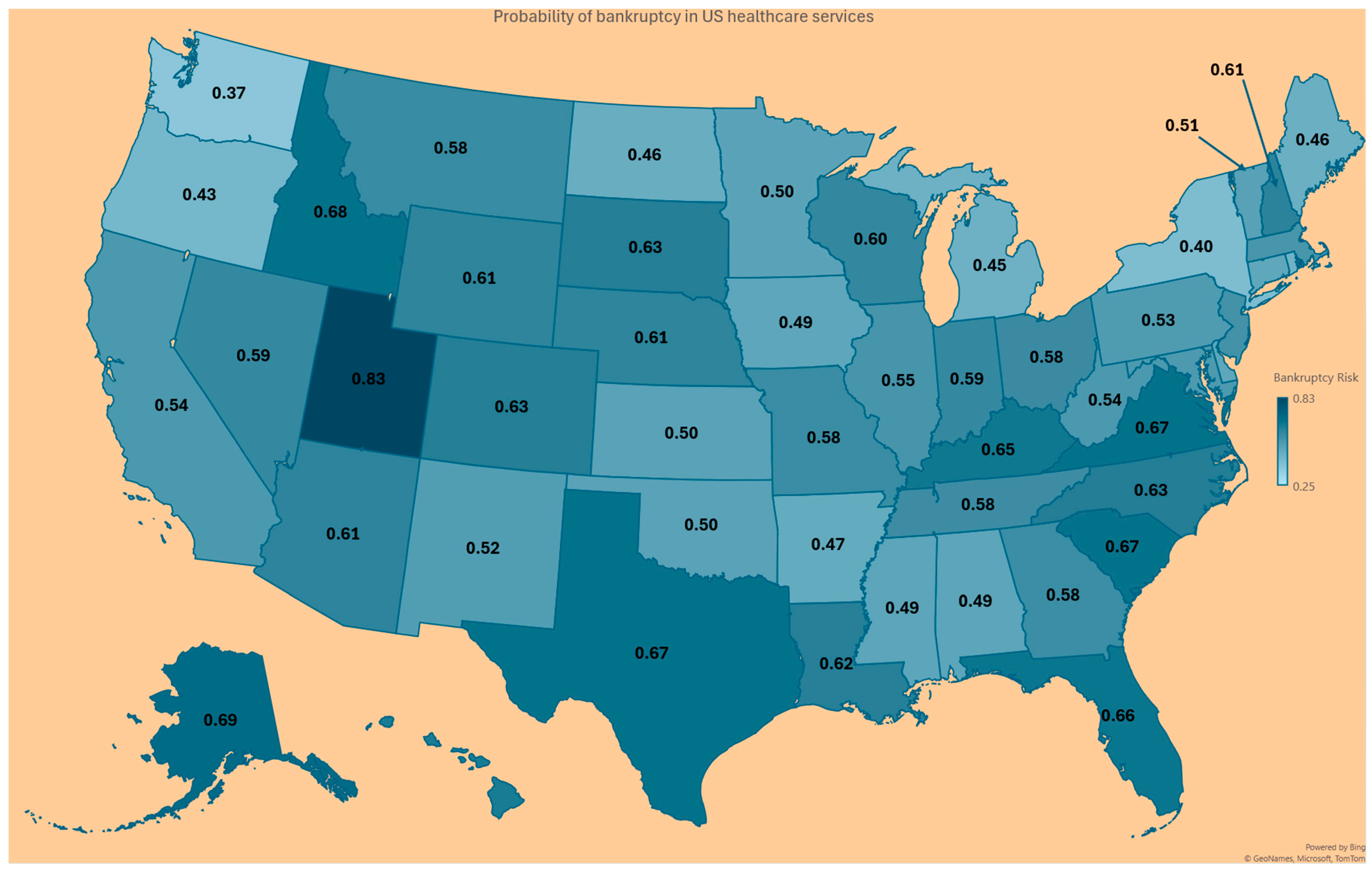
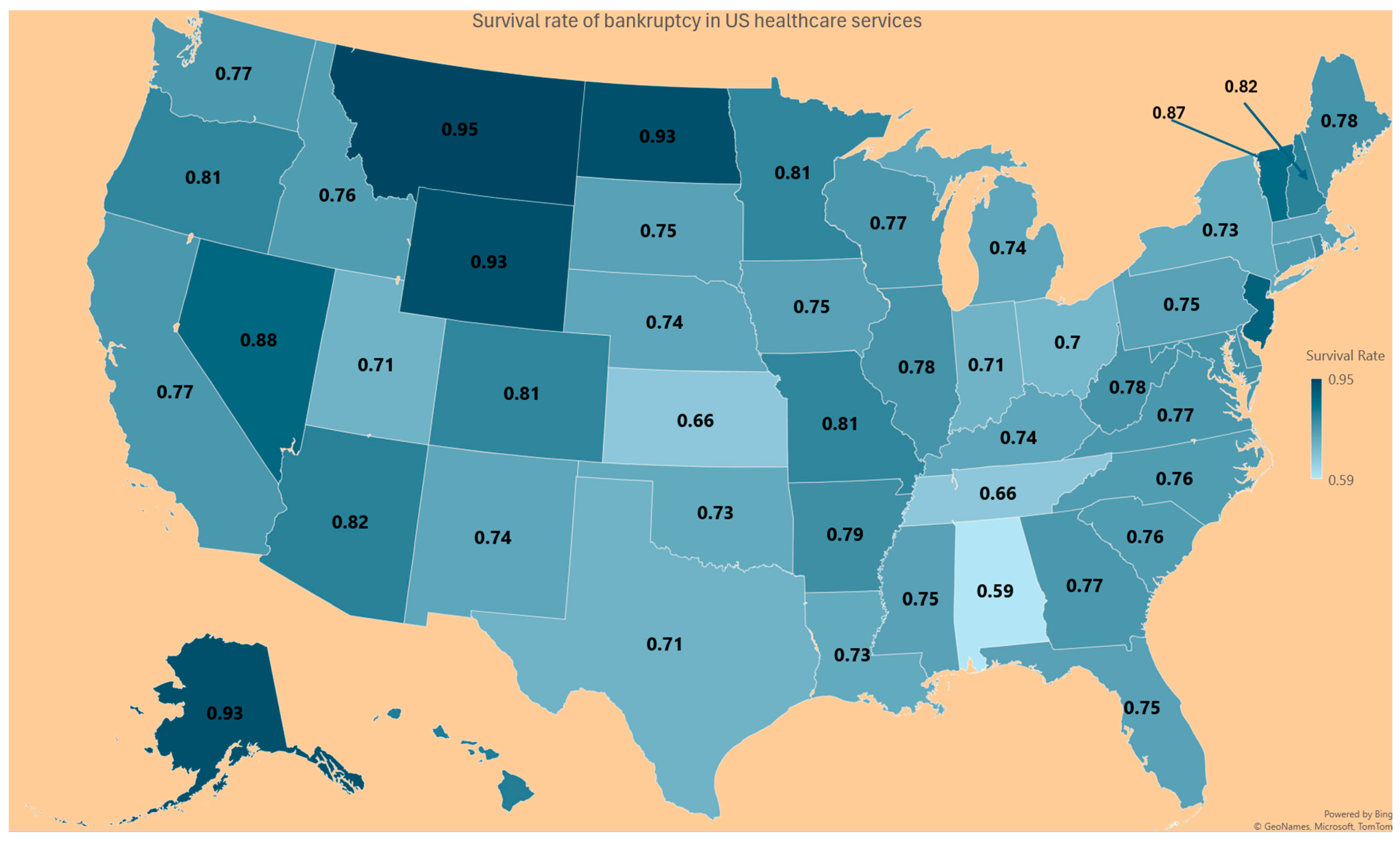
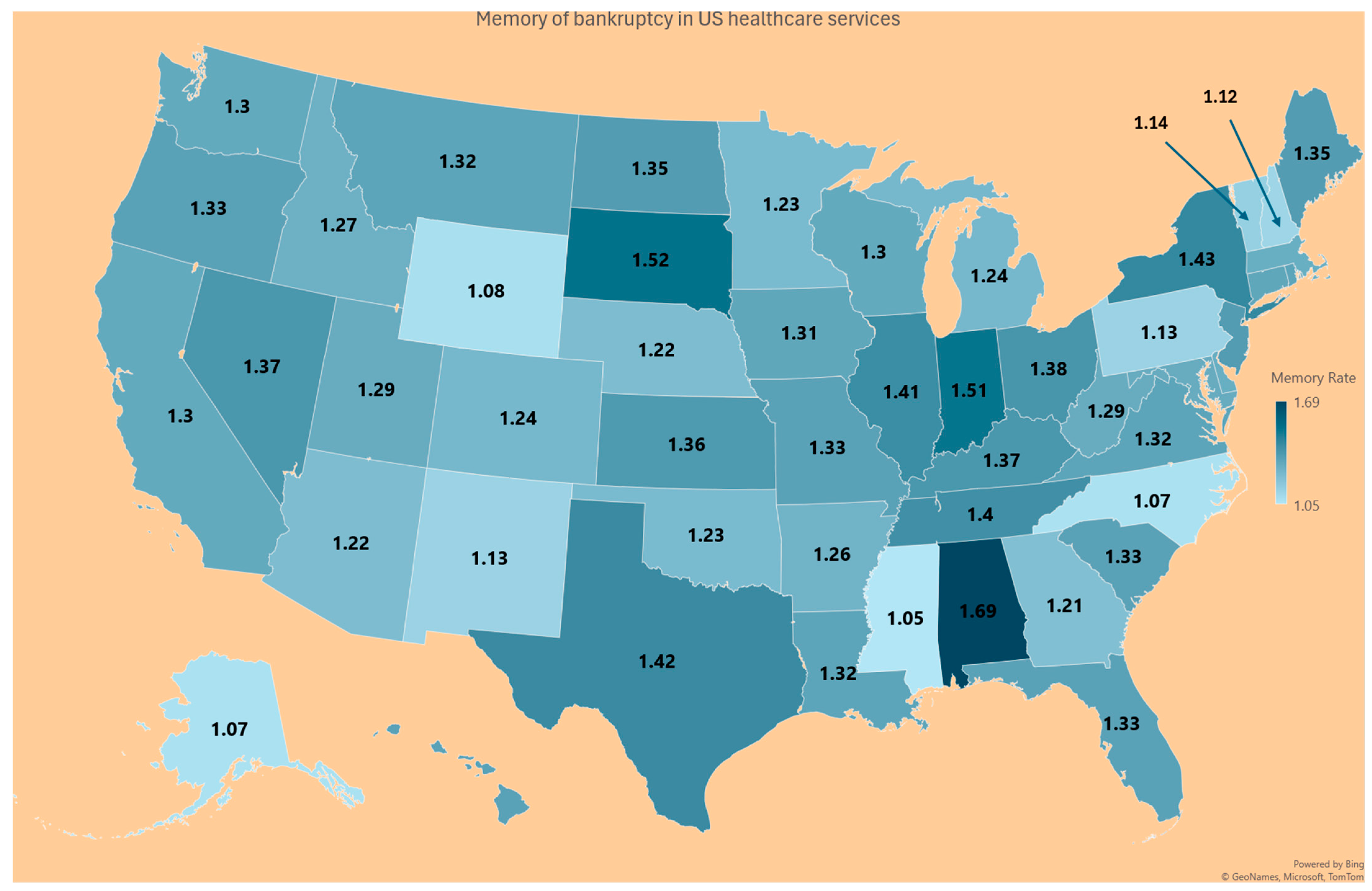
| State | Probability Prob (R < O) in (6) | Survival Rate (7) | Memory of the Finance System (8) |
|---|---|---|---|
| AK | 0.69 | 0.93 | 1.07 |
| AL | 0.49 | 0.59 | 1.69 |
| AR | 0.60 | 0.82 | 1.22 |
| AZ | 0.47 | 0.79 | 1.26 |
| CA | 0.54 | 0.81 | 1.24 |
| CO | 0.63 | 0.76 | 1.31 |
| CT | 0.49 | 0.76 | 1.32 |
| DC | 0.63 | 0.78 | 1.28 |
| DE | 0.49 | 0.75 | 1.33 |
| FL | 0.66 | 0.77 | 1.3 |
| GA | 0.58 | 0.83 | 1.21 |
| HI | 0.64 | 0.75 | 1.33 |
| IA | 0.49 | 0.76 | 1.31 |
| ID | 0.68 | 0.78 | 1.27 |
| IL | 0.55 | 0.71 | 1.41 |
| IN | 0.59 | 0.66 | 1.51 |
| KS | 0.50 | 0.74 | 1.36 |
| KY | 0.65 | 0.73 | 1.37 |
| LA | 0.62 | 0.75 | 1.32 |
| MA | 0.55 | 0.78 | 1.28 |
| MD | 0.53 | 0.78 | 1.29 |
| ME | 0.46 | 0.74 | 1.35 |
| MI | 0.45 | 0.81 | 1.24 |
| MN | 0.50 | 0.81 | 1.23 |
| MO | 0.58 | 0.75 | 1.33 |
| MS | 0.49 | 0.95 | 1.05 |
| MT | 0.58 | 0.76 | 1.32 |
| NC | 0.63 | 0.93 | 1.07 |
| ND | 0.46 | 0.74 | 1.35 |
| NE | 0.61 | 0.82 | 1.22 |
| NH | 0.61 | 0.89 | 1.12 |
| NJ | 0.56 | 0.74 | 1.35 |
| NM | 0.52 | 0.88 | 1.13 |
| NV | 0.59 | 0.73 | 1.37 |
| NY | 0.40 | 0.7 | 1.43 |
| OH | 0.58 | 0.73 | 1.38 |
| OK | 0.50 | 0.81 | 1.23 |
| OR | 0.42 | 0.75 | 1.33 |
| PA | 0.53 | 0.89 | 1.13 |
| PR | 0.52 | 0.8 | 1.25 |
| RI | 0.44 | 0.76 | 1.32 |
| SC | 0.67 | 0.75 | 1.33 |
| SD | 0.63 | 0.66 | 1.52 |
| TN | 0.58 | 0.71 | 1.4 |
| TX | 0.67 | 0.71 | 1.42 |
| UT | 0.83 | 0.77 | 1.29 |
| VA | 0.67 | 0.76 | 1.32 |
| VT | 0.51 | 0.87 | 1.14 |
| WA | 0.37 | 0.77 | 1.3 |
| WI | 0.60 | 0.77 | 1.3 |
| WV | 0.54 | 0.78 | 1.29 |
| WY | 0.61 | 0.93 | 1.08 |
5. Discussion
Limitations and Future Research
6. Conclusions
Author Contributions
Funding
Informed Consent Statement
Data Availability Statement
Acknowledgments
Conflicts of Interest
References
- Aitchison, J., and J. Brown. 1957. Lognormal Frequency structure: With Special Reference to Its Uses in Economics. Cambridge: Cambridge University Press. [Google Scholar]
- Almuqrin, Muqrin A. 2024. Bayesian and non-Bayesian inference for the compound Poisson log-normal model with application in finance. Alexandria Engineering Journal 90: 24–43. [Google Scholar] [CrossRef]
- Altman, El I. 1968. Financial ratios, discriminant analysis and the prediction of corporate bankruptcy. The Journal of Finance 23: 589–609. [Google Scholar] [CrossRef]
- Altman, El I. 2018. Applications of distress prediction models: What have we learned after 50 years from the Z-score models? International Journal of Financial Studies 6: 70. [Google Scholar] [CrossRef]
- American Hospital Association. 2022. Massive Growth in Expenses and Rising Inflation Fuel Continued Financial Challenges for America’s Hospitals and Health Systems. Cost of Caring Report. Available online: https://www.aha.org/guidesreports/2023-04-20-2022-costs-caring (accessed on 12 May 2024).
- American Hospital Association. 2024. America’s Hospitals and Health Systems Continue to Face Escalating Operational Costs and Economic Pressures as They Care for Patients and Communities. Available online: https://www.aha.org/system/files/media/file/2024/05/Americas-Hospitals-and-Health-Systems-Continue-to-Face-Escalating-Operational-Costs-and-Economic-Pressures.pdf (accessed on 23 May 2024).
- Barandela, Ricardo, Rosa M. Valdovinos, J. Salvador Sánchez, and Francesc J. Ferri. 2004. The imbalanced training sample problem: Under or over sampling? In Structural, Syntactic, and Statistical Pattern Recognition: Joint IAPR International Workshops, SSPR 2004 and SPR 2004, Lisbon, Portugal, 18–20 August 2004. Proceedings. Berlin/Heidelberg: Springer, pp. 806–14. [Google Scholar]
- Beauvais, Bradley, Zo Ramamonjiarivelo, Jose Betancourt, John Cruz, and Lawrence Fulton. 2023. The Predictive Factors of Hospital Bankruptcy—An Exploratory Study. Healthcare 11: 165. [Google Scholar] [CrossRef] [PubMed]
- Bellovary, Jodi L., Don E. Giacomino, and Michael D. Akers. 2007. A review of bankruptcy prediction studies: 1930 to present. Journal of Financial Education 33: 1–42. [Google Scholar]
- Blumenfeld, Dennis. 2001. Operations Research Calculations Handbook. Boca Raton: CRC Press. [Google Scholar]
- Carroll, Nathan W., Amy Y. Landry, Cathleen O. Erwin, Philip J. Cendoma, and Robert J. Landry, III. 2021. Factors Related to Hospital Bankruptcy: 2007–2019. Journal of Accounting and Finance 21. [Google Scholar]
- Chattamvelli, Rajan, and Ramalingam Shanmugam. 2022. Continuous Distributions in Engineering and the Applied Sciences—Part I. Berlin/Heidelberger: Springer Nature. [Google Scholar]
- Citterio, Alberto. 2024. Bank failure prediction models: Review and outlook. Socio-Economic Planning Sciences 92: 101818. [Google Scholar] [CrossRef]
- Definitive. 2024. Available online: https://www.ncbi.nlm.nih.gov/pmc/articles/PMC9858769/ (accessed on 15 May 2024).
- Dobkin, Carlos, Amy Finkelstein, Raymond Kluender, and Matthew J. Notowidigdo. 2018. The economic consequences of hospital admissions. American Economic Review 108: 308–52. [Google Scholar] [CrossRef]
- Dubas-Jakóbczyk, Katarzyna, Costase Ndayishimiye, Przemysław Szetela, and Christoph Sowada. 2024. Hospitals’ financial performance across European countries: A scoping review protocol. BMJ Open 14: e077880. [Google Scholar] [CrossRef]
- Enumah, Samuel J., and David C. Chang. 2021. Predictors of financial distress among private US hospitals. Journal of Surgical Research 267: 251–59. [Google Scholar] [CrossRef]
- Gangwani, Divya, and Xingquan Zhu. 2024. Modeling and prediction of business success: A survey. Artificial Intelligence Review 57: 44. [Google Scholar] [CrossRef]
- Gholampoor, Hadi, and Majid Asadi. 2024. Risk Analysis of Bankruptcy in the US Healthcare Industries Based on Financial Ratios: A Machine Learning Analysis. Journal of Theoretical and Applied Electronic Commerce Research 19: 1303–20. [Google Scholar] [CrossRef]
- Gomes, Conceição, Filipa Campos, Cátia Malheiros, and Luís Lima Santos. 2023. Restaurants’ Solvency in Portugal during COVID-19. International Journal of Financial Studies 11: 63. [Google Scholar] [CrossRef]
- Greenland, Sander. 2024. Regression methods for epidemiological analysis. In Handbook of Epidemiology. New York: Springer, pp. 1–76. [Google Scholar]
- Gruszczyński, Marek. 2019. On unbalanced sampling in bankruptcy prediction. International Journal of Financial Studies 7: 28. [Google Scholar] [CrossRef]
- Hillegeist, Stephen A., Elizabeth K. Keating, Donald P. Cram, and Kyle G. Lundstedt. 2004. Assessing the probability of bankruptcy. Review of Accounting Studies 9: 5–34. [Google Scholar] [CrossRef]
- IBM SPSS Statistics for Windows. 2024. Version 28.0. Armonk: IBM Corp. Available online: https://www.ibm.com/products/spss-statistics (accessed on 15 May 2024).
- Issa, Samar, Gulhan Bizel, Sharath K. Jagannathan, and Sri Sarat Chaitanya Gollapalli. 2024. A Comprehensive Approach to Bankruptcy Risk Evaluation in the Financial Industry. Journal of Risk and Financial Management 17: 41. [Google Scholar] [CrossRef]
- Ivanova, Mariya N., Henrik Nilsson, and Milda Tylaite. 2024. Yesterday is history, tomorrow is a mystery: Directors’ and CEOs’ prior bankruptcy experiences and the financial risk of their current firms. Journal of Business Finance & Accounting 51: 595–630. [Google Scholar]
- Keele, Luke, and Nathan J. Kelly. 2006. Dynamic models for dynamic theories: The ins and outs of lagged dependent variables. Political Analysis 14: 186–205. [Google Scholar] [CrossRef]
- Koptseva, Elena P., Liudmila P. Paristova, and Ekaterina G. Sycheva. 2022. Model for determining the probability of airline bankruptcy. Transportation Research Procedia 61: 164–70. [Google Scholar] [CrossRef]
- Kyoud, Ayoub, Cherif El Msiyah, and Jaouad Madkour. 2023. Modelling systemic risk in Morocco’s banking system. International Journal of Financial Studies 11: 70. [Google Scholar] [CrossRef]
- Landry, Amy Yarbrough, and Robert J. Landry III. 2009. Factors associated with hospital bankruptcies: A political and economic framework. Journal of Healthcare Management 54: 252–71. [Google Scholar] [CrossRef]
- Lawrence, Judy Ramage, Surapol Pongsatat, and Howard Lawrence. 2015. The use of Ohlson’s O-score for bankruptcy prediction in Thailand. Journal of Applied Business Research 31: 2069. [Google Scholar] [CrossRef]
- Li, Xiang. 2024. Comparing Linear Regression and Decision Trees for Housing Price Prediction. Paper presented at 2023 International Conference on Data Science, Advanced Algorithm, and Intelligent Computing (DAI 2023), Lucknow, India, July 14–15; Amsterdam: Atlantis Press, pp. 77–84. [Google Scholar]
- Lien, Donald. 1986. Moments of ordered bivariate log-normal frequency structures. Economics Letters 20: 45–47. [Google Scholar] [CrossRef]
- Lien, Donald. 2005. On the minimum and maximum of bivariate lognormal random variables. Extremes 8: 79–83. [Google Scholar] [CrossRef]
- Microsoft Mathematics-4. n.d. Redmond: Microsoft. Available online: https://www.microsoft.com/en-us/ (accessed on 15 May 2024).
- Muñoz-Izquierdo, Nora, María-del-Mar Camacho-Miñano, María-Jesús Segovia-Vargas, and David Pascual-Ezama. 2019. Is the external audit report useful for bankruptcy prediction? Evidence using artificial intelligence. International Journal of Financial Studies 7: 20. [Google Scholar] [CrossRef]
- Nawajah, Inad, Hassan Kanj, Yehia Kotb, Julian Hoxha, Mouhammad Alakkoumi, and Kamel Jebreen. 2024. Bayesian regression analysis using median rank set sampling. European Journal of Pure and Applied Mathematics 17: 180–200. [Google Scholar] [CrossRef]
- Ohlson, James A. 1980. Financial ratios and the probabilistic prediction of bankruptcy. J. Account. Res. 18: 109–31. [Google Scholar] [CrossRef]
- Payerchin, Richard. 2024. Health Care Bankruptcies in 2023 Reach Highest Level in Five Years. Medical Economics. February 9. Available online: https://www.medicaleconomics.com/view/health-care-bankruptcies-in-2023-reach-highest-level-in-five-years (accessed on 22 May 2024).
- Phan, Linh N., Mario G. Beruvides, and Victor G. Tercero-Gómez. 2024. Statistical Analysis of Minsky’s Financial Instability Hypothesis for the 1945–2023 Era. Journal of Risk and Financial Management 17: 32. [Google Scholar] [CrossRef]
- Prusak, Błażej. 2018. Review of research into enterprise bankruptcy prediction in selected central and eastern European countries. International Journal of Financial Studies 6: 60. [Google Scholar] [CrossRef]
- Ramamonjiarivelo, Zo H. 2013. Public hospitals in peril: Factors associated with financial distress. In Academy of Management Proceedings. Briarcliff Manor: Academy of Management, vol. 2013, p. 12764. [Google Scholar]
- Ramamonjiarivelo, Zo, Robert Weech-Maldonado, Larry Hearld, Rohit Pradhan, and Ganisher K. Davlyatov. 2020. The privatization of public hospitals: Its impact on financial performance. Medical Care Research and Review 77: 249–60. [Google Scholar] [CrossRef]
- Rastogi, Sonal. 2024. Rural Health Care in the Age of Hospital Bankruptcies. Emory Bankruptcy Developments Journal 40: 215. [Google Scholar]
- Ratnasari, I., N. Nugraha, and I. Sutardiyanta. 2024. Predicting Bankruptcy of Pharmaceutical Companies Using the Altman Z-Score and Grover Methods. Accounthink: Journal of Accounting and Finance 9. [Google Scholar]
- Santoso, Nurilen Wuri, Ratih Kusumawardhani, and Alfiatul Maulida. 2024. Comparative Analysis of The Altman, Ohlson, and Zmijewski Models to Predict Financial Distress During the COVID-19 Pandemic. MAKSIMUM: Media Akuntansi Universitas Muhammadiyah Semarang 14: 13–21. [Google Scholar] [CrossRef]
- Shi, Yin, and Xiaoni Li. 2021. Determinants of financial distress in the European air transport industry: The moderating effect of being a flag-carrier. PLoS ONE 16: e0259149. [Google Scholar] [CrossRef] [PubMed]
- Thoimopoulos, Nick T., and A. Longinow. 1984. Bivariate Lognormal Probability Frequency structure. Journal of Structural Engineering 110: 3045–49. [Google Scholar] [CrossRef]
- van Dijk, Tessa S., Martijn Felder, Richard T. J. M. Janssen, and Wilma K. van der Scheer. 2024. For better or worse: Governing healthcare organizations in times of financial distress. Sociology of Health & Illness 46: 926–947. [Google Scholar]
- Wieczorek-Kosmala, Monika. 2021. COVID-19 impact on the hospitality industry: Exploratory study of financial-slack-driven risk preparedness. International Journal of Hospitality Management 94: 102799. [Google Scholar] [CrossRef]
- Xu, Yong, Gang Kou, Yi Peng, Kexing Ding, Daji Ergu, and Fahd S. Alotaibi. 2024. Profit-and risk-driven credit scoring under parameter uncertainty: A multi objective approach. Omega 125: 103004. [Google Scholar] [CrossRef]
- Zmijewski, Mark E. 1984. Methodological Issues Related to the Estimation of Financial Distress Prediction Models. Journal of Accounting Research 22: 59–82. [Google Scholar] [CrossRef]


Disclaimer/Publisher’s Note: The statements, opinions and data contained in all publications are solely those of the individual author(s) and contributor(s) and not of MDPI and/or the editor(s). MDPI and/or the editor(s) disclaim responsibility for any injury to people or property resulting from any ideas, methods, instructions or products referred to in the content. |
© 2024 by the authors. Licensee MDPI, Basel, Switzerland. This article is an open access article distributed under the terms and conditions of the Creative Commons Attribution (CC BY) license (https://creativecommons.org/licenses/by/4.0/).
Share and Cite
Shanmugam, R.; Beauvais, B.; Dolezel, D.; Pradhan, R.; Ramamonjiarivelo, Z. The Probability of Hospital Bankruptcy: A Stochastic Approach. Int. J. Financial Stud. 2024, 12, 85. https://doi.org/10.3390/ijfs12030085
Shanmugam R, Beauvais B, Dolezel D, Pradhan R, Ramamonjiarivelo Z. The Probability of Hospital Bankruptcy: A Stochastic Approach. International Journal of Financial Studies. 2024; 12(3):85. https://doi.org/10.3390/ijfs12030085
Chicago/Turabian StyleShanmugam, Ramalingam, Brad Beauvais, Diane Dolezel, Rohit Pradhan, and Zo Ramamonjiarivelo. 2024. "The Probability of Hospital Bankruptcy: A Stochastic Approach" International Journal of Financial Studies 12, no. 3: 85. https://doi.org/10.3390/ijfs12030085