Two Investment Options for Bearish ETF Investors: Inverse ETF and Shorting ETF

Abstract

A high liquidity, low expense ratio and the possibility to conduct arbitrage allow exchange-traded funds (ETFs) to be used for short sales. Bearish investors can also buy inverse ETFs. This paper aims to outline two investment approaches for bearish ETF investors and the differences between these two approaches; it also aims to examine the relationship between price and an indicator of volume and evaluate the final positions in selected ETFs in selected periods. Short ETFs dominate in simplicity, flexibility, paying out dividends and especially in the limited size of the loss. On the other hand, their structure, which demands daily rebalancing, causes substantial deviation from the benchmark in the long-term and leads to a higher expense ratio, and lower liquidity increases bid-ask spreads. Negative aspects of ETF short selling lie in unlimited loss, high borrowing costs, the need for margin accounts, variability of loan fees and the possibility of a transaction recall by the lender. On the contrary, margin operations enable potentially higher appreciation of capital by generating rebate rates. Our results show that with the decrease in value of the most used ETFs, short interest is growing for those funds where there is a very strong negative correlation implying hedging tendencies. Short selling proved to be a more advantageous strategy in the observed period of market downturn, as well as in 2011–2017, due to negative returns, however, by applying margin trading inverse ETFs turned out to make less losses. Sector-oriented inverse ETFs are the exception, where the largest differences between these two strategies are recorded. However, the final conclusion of the suitability of one of the analyzed strategies depends on the market volatility and the direction of the market itself.

1. Introduction

Great success of index investing by the traditional index mutual funds led to the creation of index funds that are traded on the stock exchange, the exchange-traded funds (ETFs). These types of funds offer investors even bigger benefits than traditional index funds. They are particularly attractive for investors due to wider diversification opportunities, a large number of different types of ETFs in terms of their underlying assets or their sectoral focus, as well as due to the multiple ways of benchmark replicating. ETFs exhibit significantly lower levels of expense ratio compared to other instruments of collective investment and they are also more tax efficient, as there is no taxable event during the creation/redemption in-kind process, as they distribute capital gains only very rarely. ETFs are traded continuously throughout trading hours, which leads to much higher liquidity. Issuance of their stocks allows investors to set limit orders, to use them for collateral trading and forwards, to conduct arbitrage when the price on the secondary market deviates from the net asset value of the ETF’s underlying assets and to use them for short sales. However, investors who want to invest in ETFs and have bearish expectations and do not only have to use forwards without direct borrowing of shares; they also have an option to create a short position, the inverse ETF. This paper focuses on comparing these two strategies of being short in ETFs, we balance their advantages and disadvantages, describe how they work, discuss the possible risks associated with these strategies and describe the structure of short ETFs. We also show how inverse ETFs’ returns deviate from the returns of normal ETFs in the long-run, examine the relationship between short ETFs´ price and their interest, and between the price of inverse ETFs with the same reference benchmark and their trading volume. Finally, we evaluate the performance and the suitability of using these two strategies for bearish investors for investing into ETFs in the selected period. The data for this study are taken from Bloomberg and the ETF Database.

The first section of this paper presents several views and research findings on ETF short selling and inverse ETFs. Then, we outline the methodology of our research with definition of the funds in the observation sample. The second section presents the results and the summary of these results is provided in the discussion.

2. Literature Review

Several publications dealing with either inverse ETFs or short ETFs can be found in the literature. Abner 2010 outlines the main features of inverse ETFs, otherwise known as short ETFs. Accounts, such as individual retirement accounts, are not able to gain such a market access that would protect them in case of market falls, while a purchase of inverse ETFs provides investors with downside market protection. One of the significant benefits of inverse ETFs compared to standard ETF short selling is the ability to limit certain risks. The reason is that by selling an ETF short the investor is exposed to practically unlimited position growth, while in the case of an inverse ETF, the loss is limited by the volume of funds invested into the position. Moreover, the inverse ETFs invest in other segments of financial market. In addition to stock indices, which may track the performance of particular sectors or regions, inverse ETFs may also invest into basic commodities, real estate, interest rates, precious metals or world currencies (Kmeťko 2012). The purchase of stocks on capital market is associated with the risk of a decrease of the stock’s value as a result of price changes in other parts of the financial market. On the other hand, with regards to hedging the portfolio against a market decline, short ETFs appear to have more advantages compared to techniques using derivatives; when speculating on the market decline for a period that is longer than the maturity of the derivate, the investor must bear additional costs associated with contract rollout and the price might change as well. Lydon (2010) states that the biggest advantage of short ETFs is their simplicity. Such a fund could be easily bought without complicated borrowing and investors do not need to have margin accounts. At the same time, however, he draws attention to two important aspects that we should be aware of with regards to inverse, or leveraged inverse ETFs:

• their possible hyper-volatility;
• their inappropriateness for the buy-and-hold strategy.

In the case of inverse leveraged exchange-traded funds that deliver returns that are two or three times higher than the opposite of market yield, we can observe significant price fluctuations even within one day. Profitability of these funds stray from their 200-day moving averages and a change of more than 20% over single day is not rare. Due to their daily reset they sometimes deviate from their benchmarks over time even though they still meet their stated goal. This is the reason why they are not suitable for long-term investment like the buy-and-hold strategy. Over the long-term, inverse ETFs with high levels of leverage, i.e., the funds that deliver three times the opposite returns, tend to converge to zero (Carver 2009). This also applies to the short ETFs with a lower leverage in cases of high volatility of the underlying index. However, the results of Guedj et al. (2010) surprisingly show that investors hold their leveraged ETFs for a rather long period, more than three months, while the original invested amount of some investors decreased by 3% in a few weeks, which corresponds to a 50% annualized yield. These authors also mention the inverse open-end mutual funds that were first offered by the ProFunds Group in 1997and similarly inverse ETFs that reset their portfolios on a daily basis to gain the required exposure.

Another strand of research (Hessel et al. 2018) has explored the strategy of concurrent shorting of an inverse ETF and a leveraged ETF with the same underlying index. These authors applied this strategy to six markets and they concluded that the direction of the movements of the underlying index, that is either upward or downward moves, is not decisive for profitability. However, if the index tends to return to its mean value, the strategy is profitable, whereas if the index moves in a trend the strategy generates a loss. The utilization of the strategy with a pair of ETFs brought an average monthly yield of 1% in four markets.

Investors´ speculations on a decrease in stock prices are realized not only by using inverse ETFs but in fact largely by ETF short selling. While the level of interest in short-selling in the case of international ETFs appears to be unusually low, the investor’s interest is abnormally high within sector-oriented ETFs (Madura and Ngo 2008). Compared to individual stocks, short interest in exchange-traded funds is on average more than ten times higher, with higher short interest in ETFs with higher trading volumes and lower market capitalization, as well as in international funds copying indexes with tradable derivatives. Shorting ETFs is preferred by arbitrageurs due to their liquidity and as due to their ability to avoid the constraints associated with individual stocks (Li and Zhu 2016). Moreover, new ETFs might be only be created with intention of short selling and can then be used for the creation of short exposure to those stocks whose short sales alone would be too costly. It follows that with increasing difficulty of shorting individual stocks, the volume of ETF short sales rises. The analysis of Hughen and Ma (2013) suggests that the level of short selling is also influenced by the creation/redemption in-kind process. They show that exchange-traded funds with high levels of short sales experience positive excess returns in contrast to individual stocks. Such returns are also made by ETFs tracking foreign stock indices with low levels of short sales and is usually caused by higher foreign stock prices. The determinants of the short interest ratio of stocks in general were studied by Brent et al. (1990) based on three groups of motives: tax, speculative and arbitrary motives. The tax motive was studied through an analysis of seasonal fluctuations in interest rate; a significant growth of this variable at the end of the year and a subsequent significant decline at the beginning of the year indicates the existence of a tax motive. The arbitrary, or hedge motive was investigated through the existence (non-existence) of a negotiable option, the existence (non-existence) of convertible securities and the beta coefficient. High beta shares are attractive as a hedging instrument due to the tendency to achieve a high correlation with the market (McDonald and Baron 1973). The speculative motive in investor behavior was examined by using the variable of average variation coefficient and the monthly return on shares for the previous year. De Bondt and Thaler (1985) suggest that short interest will rise after increases of stock prices in the previous period, while the short interest will decrease if the stock prices fell during the previous period.

3. Methodology and Data

This article focuses on examination of two ways of investing into ETFs when speculating on market decline, investing long into inverse ETFs and ETF short selling. We describe the differences between these two strategies. For this purpose, we have chosen 12 exchange-traded funds, as well as 12 inverse exchange-traded funds that have the same reference index, the inverse ETFs aim to deliver a daily return 100% opposite to the daily return of these reference indexes. Our sample includes funds with diverse underlying indexes. From the perspective of market capitalization, we examine ETFs with reference indexes from the following categories:

• small-cap, such as Russel 2000 Index, S&P SmallCap 600 Index;
• mid-cap, such as S&P 400 MidCap Index;
• large-cap, such as S&P 500 Index.

Additionally, we have chosen some indices that are sector-oriented, for example targeted at the finance sector, such as the Dow Jones U.S. Financials Index, at companies dealing with the extraction and processing of oil and gas (Dow Jones U.S. Oil & Gas Index) or at companies engaged in other sectors or industries, such as the Alerian MLP Infrastructure Total Return Index, which is a composite of energy infrastructure master limited partnerships, capped, float-adjusted, capitalization-weighted indexes, whose constituents earn the majority of their cash flow from midstream activities involving energy commodities, or the Dow Jones U.S. Basic Materials Index. From a territorial point of view, indexes are primarily focused on the US stock market. Some funds, however, invest in companies from the Chinese stock market, such as one fund copying the performance of FTSE/Xinhua China 25 Index, or companies that are traded on the European, Australasian and Far Eastern stock markets, such as the ETF tracking the MSCI EAFE Index. The majority of selected “classic” exchange-traded funds are provided by BlackRock, formally known as Barclays, which is globally the biggest ETF issuer with a nearly 40% share of the global market with these instruments. Others are managed by companies such as Invesco Powershares, State Street Global Advisors, or UBS. All selected short ETFs are, except for one that is provided by UBS, issued by ProShares, which is, as noted below, one of the three leading companies in the sphere of leverage and inverse ETFs. For ease of reference in the article, we list funds under their abbreviations. The classical funds´ abbreviations, together with the indexes they copy, are presented in Table 3. The same indexes represent benchmarks for the relevant inverse ETFs.

For our examination we have used daily as well as quarterly data for the period from 2011 to 2017. Bloomberg, along with the ETF Database were our main sources of data. In order to find the so-called inverse “twins” to functioning funds on the market, we had to choose this period, because the inverse ETF is a very young instrument. We processed the data to determine quarterly profitability in terms of both the “classic” exchange-traded funds and inverse exchange-traded funds, standard deviation of these returns and total return for the observed period. We have also used data on trading volumes as well as on the volume of short sales in the form of indicators of short interest and short interest ratio, respectively. To examine the relationship between the ETFs´ prices and their short interests, and the inverse ETFs’ prices and their trading volumes, we have used the correlation method, and for other analyses we have applied mathematical and statistical methods.

We evaluate the profitability or loss of utilization of the stated instruments, first on a quarterly basis during the period of 2011–2017 and subsequently in the period of three months of market decline from September 2008 on a daily basis. We compare appreciation/depreciation without any corrections on the one hand and the 50% short sell margin on the other.

In order to assess the suitability and profitability of the bearish strategies under consideration on downward market, we analyzed three inverse funds (and then a short-selling strategy) on a daily basis over a period of three months, from September 2008 to November 2008, when we see a nearly continuous decline in the market. For both observed periods we then calculated the applied short rebate rate of 0.5% per annum.

4. Results

Due to market volatility and asset prices fluctuations, the speculation on growth is sometimes neither advantageous and appropriate, nor sufficient. Some investors only want to protect their portfolios against falling market prices and they do so mainly by entering into term and option contracts. Other investors use, or at least try to use, this volatility to their advantage and they enter into short positions instead of long positions. To make profit on a declining market, they sell short various stocks. Thanks to their structure—they are traded on a stock exchange just like plain stocks—exchange-traded funds offer the possibility to be short in the broad market with a considerable degree of diversification. However, ETFs are a specific product which has several different forms. One of these are the inverse ETFs, the purchase of which represents yield hedging in the event of a fall in the value of assets, which the ETF tracks.

Compared to other ETFs, normally those that copy the reference index, inverse ETFs are less tax efficient, as the tax efficiency benefit disappears. The reason behind this is that, as mentioned above, these instruments use multiple term contracts, usually forwards or swaps, in order to gain the requested exposure. These derivatives do not constitute in-kind transactions, instead they are settled through funds transfers. Additionally, these types of funds are associated with higher trading costs due to the higher number of transactions and strategies that are applied to them and they are riskier in contrast to standard forms of index funds. These higher transaction costs are then reflected into the level of the expense ratio, which can also be seen on the selected sample of exchange-traded funds. While in the case of selected “classical” ETFs, the average expense ratio is 0.34%, in the case of inverse ETFs there is an average expense ratio of 0.94%.

Inverse index stocks often pose as leverage funds, which are considered risky. Leverage and inverse leverage ETFs could consequently be marked as “L x ETF”, where:

• L < 1 in the case of bear ETF;
• L > 1 in the case of bull ETF.

Ninety-eight percent of the market capitalization of these funds is covered by three companies, the ProFunds Group, Direxion Funds and Rydex Investments, which was acquired by Guggenheim Investments in 2010. These ETFs generally buy option contracts or futures options such as futures or total return swaps into their portfolio. They mostly offer a leverage of −3 to 3 and are re-rated daily. The greatest threat to the investor in the case of leverage ETFs is the volatility of the underlying securities. The problem is that while the leverage effect on the fund’s return is linear; the volatility of the underlying asset has an exponential effect on the fund’s return. For example, considering an investment horizon of three days, for an index fund in the form of 3X ETF, an increase in the value of the underlying index on the first day by 5%, and a subsequent decrease of 10% and an increase of 5% on second and third day, respectively, would amount to a loss of only 0.775%, while the invested amount in the leverage ETF fell by 7.425%.

Advisor Perspectives states that the investor should only increase the leverage if the investor’s earnings expectations are positive, and the potential impact of fees and volatility is less than the inflow of multiple profits. The recommended leverage level is between 1.5 and 2, based on an analysis of data spanning the period of over 25 years until 2009, and in the long-run a leverage level of over 3.5 is not suitable (Finlord 2016). This type of index fund usually uses swaps or other term contracts to achieve their goal, as a result they acquire the character of synthetic ETFs.

Synthetic ETFs, where the market value of swaps is derived from the performance of a copied index, are particularly interesting because they give investors access to hard-to-reach markets, and they enable investors to purchase securities whose physical purchase is either very demanding or directly impossible. ETF Provider is a standard offshore asset management unit of a bank that sells ETF shares to investors. For collected funds, the basket of securities is purchased as collateral. The revenues from this basket of securities are then swapped by the so-called Derivative Desk of the same bank for the earnings of the tracked index (FSB 2011). The asset basket emerging as collateral may or may not have any relationship to the components of the copied index.

One of the biggest risks the exchange-traded funds are exposed to is the counterparty risk. In an extreme case, the swap counterparty defaults to ensure the profitability of the index tracked by a synthetic ETF and to deliver that return to the fund based on the given term contract. Therefore, the credit risk arises from a possible default of the swap counterparty in a balanced liability to the trustee, therefore, the high level of creditworthiness of the counterparty is the essential prerequisite for the operation and life-time of synthetic ETFs. Synthetic ETFs are also subject to certain regulatory measures as a protection against this risk of counterparty swapping. For example, in the case of funds classified as UCITS, the net exposure to counterparty risk must not exceed 10% of the net asset value of the fund, which means that at least 90% of the fund’s assets must be collateralized. However, most funds voluntarily fully collate their overall exposure. If the underlying index is valued more than the collateral, this difference represents the exposure level of counterparty risk. In this case, however, when a counterparty swap is cleared, the difference is paid to the fund, and is subsequently invested into the expansion of the collateral, thereby reducing the counterparty risk completely. Conversely, if the collateral is valued more than the underlying assets of the fund, the resulting difference is paid to the counterparty. In some cases, a swap agreement is reset before 10% of the net asset value is reached, otherwise the result is performed on a daily basis (Riedl 2015). Some swap exchange-traded funds even prefer collateralization to protect investors to fully cover the value of the fund during the collapse of the collateral. The fact that the ETF is also acting as a swap counterparty encourages the emergence of systematic risk and risk of infection.

As synthetic ETFs are becoming more and more popular, the volume of assets under their management is steadily rising, even though they are not the dominant type of ETF. Within Europe, synthetic ETFs account for almost half of the stock market and they account for a boom in the market in Asia. More liberal regulation in the European market compared to the U.S. contributes to the development of this kind of ETF in Europe. While regulation of UCITS III allows the use of derivatives for investment purposes, and not just for hedging purposes, the SEC has been evaluating the use of derivatives by these types of ETFs since March 2010, thereby shifting the consideration of applications for the authorization of those funds that intend to invest heavily in derivatives (FSB 2011). Another driving engine for the development of synthetic ETFs are synergistic effects arising within the banking group if the branch of the asset management bank acts as a swap counterparty to this ETF provider.

When buying the inverse ETFs, the liquidity provider has to short that exchange-traded fund to the investor, which means that the liquidity provider is getting the long position in the given assets. The liquidity provider subsequently sells a block of some assets that are highly correlated with the long exposure, in order to hedge this exposure. The block of assets may be a block of shares, but also a variety of derivatives (Abner 2010). In order to ensure the desired yield of the short exchange-traded fund on the rolling basis, the inverse ETFs must reset their portfolio daily, like other leveraged instruments. In the case of an inverse leverage ETF, the fund must acquire exposure to a hypothetical asset value equal to several times (according to the leverage level) of its net asset value. An exchange-traded fund holds a certain amount of assets which the fund swaps with its counterparty, so that it can provide an adequate level of multiple (or opposite to the multiple) exposures to assets whose performance the ETF tracks. For example, we might expect that the short ETF delivering three-times opposite return is together with the underlying benchmark index at the level of 100 in the initial period. If the market of the index were to rise by 10% the next day, the short ETF is reduced to the level of just 70, the value of assets generating yield is −220. This means that the fund has to reduce the short exposure by 10 units of assets to generate three-times the opposite yield. Conversely, if the market were to decline by 10%, the index would drop to the level of 90, while the short ETF would rise to level of 130 and the level of assets would be at the level of 330 short units. The inverse exchange-traded fund should short additional 60 units of assets to generate three-times the exposure. The rebalancing activities of these ETFs almost always coincides with the direction of the market (Abner 2010). This daily rebalancing is, of course, associated with higher transaction costs. Moreover, the very need to carry out daily rebalancing operations increases the cost of these ETFs. The effects arising from this rebalancing are mitigated with decreasing degrees of leverage, so they are lowest for simple inverse ETFs without any leverage, and these effects are also influenced by the volatility of the reference benchmark.

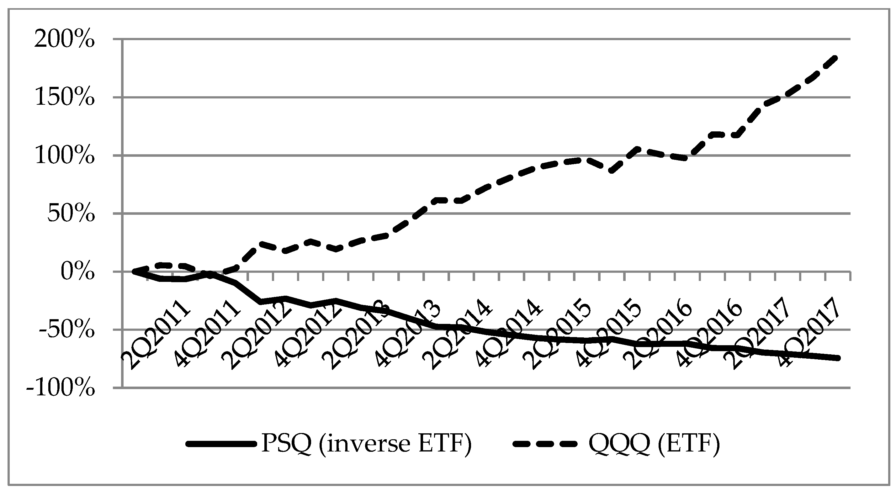
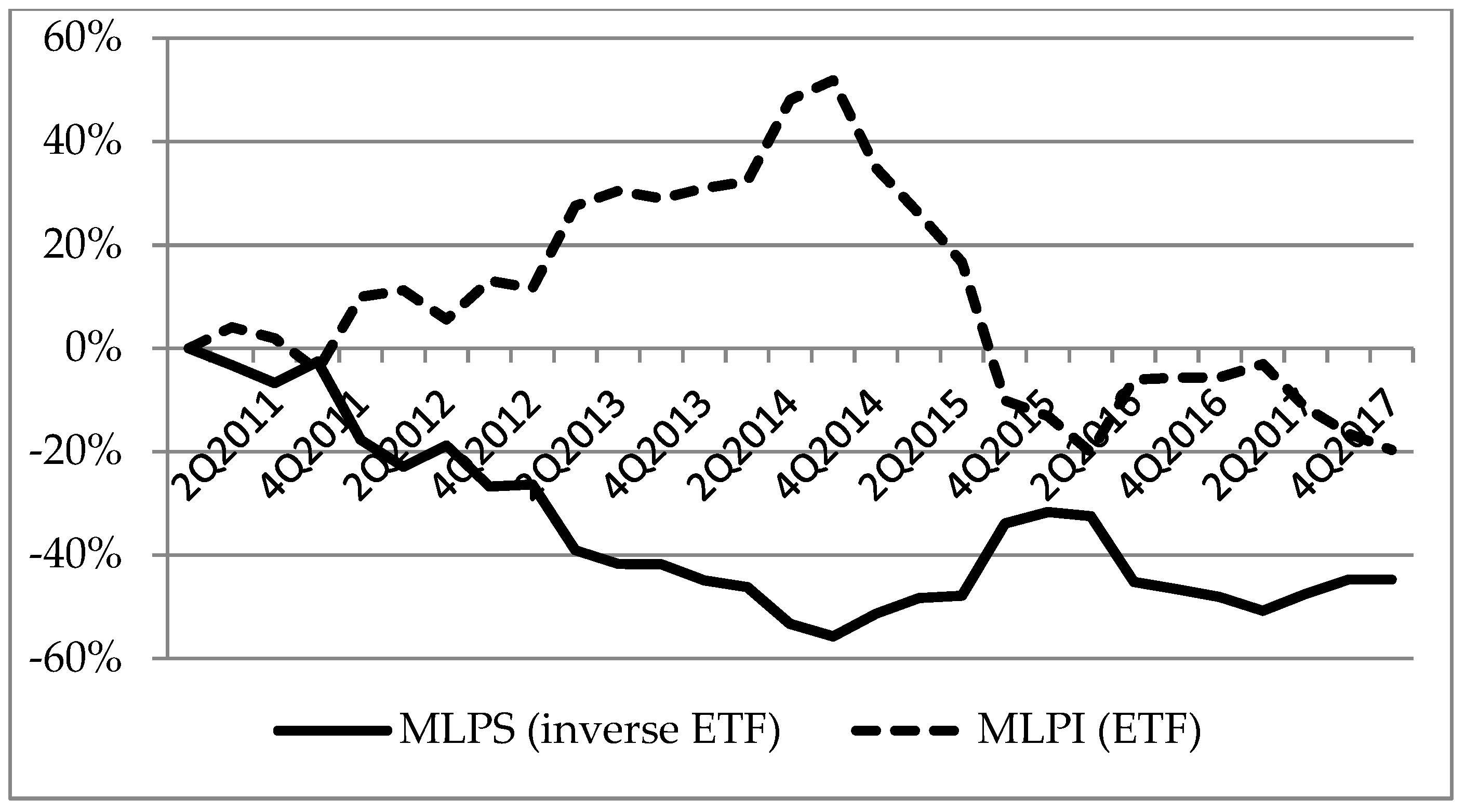
The structure of inverse exchange-traded funds does indeed provide opposite returns on a daily basis, however, in the long-run their performance does not correspond to the opposite profitability of the tracked index. Figure 1 and Figure 2 display the yield development of two selected normal exchange-traded funds from our sample and their corresponding inverse funds, measured against the base period, the end of 2010, on a quarterly basis. In terms of quarterly returns, ProShares Short QQQ deviates from the return of the classic ETF by more than 13 percentage points after 12 quarters, while UBS’s inverse ETF, which delivers the opposite return on a monthly basis, starts to deviate from the relevant ETF by more than 10 percentage points already after the first year, except for the second and third quarters of 2014. At the same time for the inverse fund ProShares Short QQQ, the total return after the observed seven years deviates from the normal ETF tracking the same index by more than 110 percentage points.

The table below compares the total returns and average quarterly returns of ETFs and 1 X inverse ETFs, which track the same benchmark index for the period 2011–2017 (see

Table 1. Comparison of ETFs and 1 X inverse ETFs with the same benchmark index for the period 2011–2017 (in %).

	ETF					Inverse ETF
	Average Quarterly Return	St. dev. of Quarterly Returns	Total Return	Expense Ratio		Average Quarterly Return	St. dev. of Quarterly Returns	Total Return	Expense Ratio
SPY	2.87	5.38	112.21	0.09	SH	−3.61	5.12	−65.58	0.89
QQQ	4.01	6.27	186.01	0.2	PSQ	−4.59	5.46	−74.34	0.95
IWM	2.73	7.84	94.86	0.2	RWM	−3.60	7.80	−67.16	0.95
IYY	2.86	5.62	110.76	0.2	DOG	−3.68	4.96	−66.30	0.95
IYF	2.94	7.52	107.78	0.44	SEF	−3.78	7.09	−68.44	0.95
EFA	0.92	6.80	20.77	0.32	EFZ	−2.17	6.63	−49.10	0.95
IJH	2.93	7.02	109.26	0.07	MYY	−3.57	6.80	−66.20	0.95
IJR	3.21	7.49	124.36	0.07	SBB	−3.97	7.22	−70.18	0.95
FXI	0.78	9.83	7.15	0.74	YXI	−2.38	10.24	−55.61	0.95
IYE	0.53	9.50	1.77	0.44	DDG	−1.55	9.48	−43.10	0.95
MLPI	−0.42	8.41	−19.63	0.85	MLPS	−1.70	8.98	−44.75	0.85
IYM	1.43	8.80	31.94	0.44	SBM	−2.19	10.32	−53.15	0.95

Source: our processing, data gathered from Bloomberg, (ETF Database n.d., http://www.etfdb.com/).

). The highest return, or alternatively the smallest loss, is recorded by inverse ETFs that are sector-oriented. These funds, along with funds from the small market capitalization category, also exhibit the highest risk, which coincides with the Fama and French three-factor model; one of these three factors is based on higher yields as well as higher volatility of shares of companies with lower market capitalization compared to shares of companies with higher market capitalization.

Another possibility of gaining exposure to the bear trend of the market or the selected portfolio of stocks is ETF short selling. Short selling allows investors to profit when the price of a financial instrument decreases. This can be achieved by allowing the investor to borrow the security and then sell it with the intent of re-purchasing the security in the future but at a lower price.

All revenues that are realized during the securities lending process are deposited by the lender who lent the security. As a result, short selling has disadvantages in comparison to investing into short ETFs, as the investor is deprived of dividend yields. The bear ETFs could pay out dividends, too, but because their portfolio includes various types of derivative contracts, these dividends come from capital gains. The value of the loan is recalculated daily, if the value of the lent securities increases, an additional deposit is required, while if the value falls, the part of the principal is returned to the borrower. When the securities are returned to the creditor, the collateral is recovered as well. While the securities are borrowed, the collateral is invested and generates revenue. In general, the lender returns part of the proceeds of the invested collateral to the borrower, as a rule, this is done based on the pre-negotiated level of the so-called rebate rate or reduced interest rate. In practice, this means that instead of the real fees for borrowing a financial instrument, the primary cost of borrowing a security is the difference between the current market interest rate and the rebate rate. The rebate rate acts as a price that equals supply and demand on the borrowing market, it may be negative in extreme cases, which means that the investor who sold it for a short period must pay the lender daily for the right to borrow the security (instead of receiving a payment from the lender as interest yield). However, this rate only partially balances the borrowing market, since the borrowing market is not centralized and it is rather on an individual agreement between the security owner and potential borrower (Fabozzi 2004).

The volume of realized short sales is assessed by short interest. It is defined as the number of shares that were sold short, but were not redeemed, thus the short position was not closed. The size of the short interest may also pose as an indicator of the market pessimism rate of a particular instrument, even though there may be other reasons than an expected fall in the price of an instrument for opening a short position. This concept of short interest corresponds to the hypothesis of overestimation, which is one of the explanations why investors open short positions. But there are other reasons for opening a short position. In the below table (see

Table 2. Correlation coefficients between ETF price and their short interest, and between inverse ETF price and their trading volume (observation period 2011–2017).

ETF	Price vs Short Interest	T-Statistic	Inverse ETF	Price vs Trading Volume	T-Statistic
SPY	−0.54	−34.66	SH	−0.08	−4.34
QQQ	−0.52	−32.89	PSQ	−0.32	−18.25
IWM	−0.84	−83.63	RWM	−0.11	−5.98
IYY	−0.08	−4.34	DOG	0.02	1.08
IYF	0.65	46.20	SEF	0.45	27.22
EFA	0.11	5.99	EFZ	0.19	10.45
IJH	0.15	8.20	MYY	0.05	2.70
IJR	−0.29	−16.37	SBB	0.08	4.34
FXI	−0.21	−11.60	YXI	0.04	2.16
IYE	0.28	15.76	DDG	0.19	10.45
MLPI	−0.18	−9.89	MLPS	0.02	1.08
IYM	−0.21	−11.60	SBM	0.18	9.89

Source: our processing, data gathered from Bloomberg, (ETF Database n.d., http://www.etfdb.com/).

) we present the correlation coefficients reflecting the relationship between the prices of traditional ETFs and the level of short selling and between inverse ETF prices and their trading volumes calculated using data on a daily basis for the period 2011–2017. For normal exchange-traded funds, which are the most well-known and traded ETFs, there is a strong negative correlation. This could imply that these funds are sold short with the intention to hedge the portfolios, because with the fall in ETF prices the level of short sales is growing. For other funds this correlation is weaker, and in some cases there is even a positive correlation. One fund, the sector-oriented ETF tracking the performance of US companies operating in the financial sector, exhibits conversely very strong positive correlation. The inverse ETF, whose reference benchmark is the same index, also displays a particularly high correlation between its price and trading volume, but this could indicate that this ETF is used to avert the drop in the prices of relevant assets. However, a slightly positive correlation is also experienced by other inverse ETFs, especially those that are sector-oriented. On the other hand, low negative correlation is found for those ETFs that track the most famous indexes as their reference benchmark, suggesting that these exchange-traded funds are more often used for speculative trades. The strength of the relationship between the above-mentioned variables was determined by the correlation coefficient, which we tested by T-statistics. Except for two cases, the DOG and MLPS funds, the correlation coefficient proved to be relevant at a significance level of 0.05.

The short selling level can also be analyzed through the short interest rate. The rising value then indicates that the value of the instrument will drop, while the decreasing value of this variable indicates that the value of the instrument will increase. Fundamental analysis sees the bear trend in the rising short interest ratio value because of its relationship with the instrument’s price. Conversely, technical analysis considers short interest ratio as an indicator of the bull market due to the relationship with the future demand for the instrument due to the termination of an open short position.

This indicator also determines how many days are needed for short sellers to close all their short positions when the price of the instrument starts to grow. A low value indicates that there are expectations of a drop or stagnation of the instrument’s rate. Conversely, if the short interest ratio increases, it takes longer to close the short position, leading to a higher risk of a short squeeze. The threshold value is seven days or more (Taulli 2011). The average short interest ratios of selected ETFs are presented below (see

Table 3. Average short interest ratio of ETFs, their benchmark indexes and median of differences in quarterly returns between ETFs and inverse ETFs in the period 2011–2017.

ETF Fund	Average Short Interest Ratio	Benchmark Index	Median of Differences in Quarterly Returns	Median of Differences with Margin 50%	Median of Difference when Rebate Rate 0.5% p.a.
SPY	2.2550	S&P 500 Index	−0.95	2.38	2.26
QQQ	1.7580	Nasdaq 100 Index	−0.94	3.64	3.52
IWM	3.6776	Russell 2000 Index	−1.29	2.25	2.12
IYY	0.9861	Dow Jones Industrial Average Index	−1.34	1.99	1.87
IYF	2.2091	Dow Jones U.S. Financials Index	−1.17	1.63	1.51
EFA	1.7044	MSCI EAFE Index	−1.35	−0.06	−0.18
IJH	1.7548	S&P MidCap 400 Index	−1.02	2.64	2.51
IJR	3.2277	S&P SmallCap 600 Index	−1.18	2.02	1.90
FXI	1.9541	FTSE/Xinhua China 25 Index	−2.50	1.31	1.18
IYE	1.3445	Dow Jones U.S. Oil & Gas Index	−1.68	−1.12	−1.25
MLPI	0.6289	Alerian MLP Infrastructure Total Return Index	−2.62	−2.59	−2.71
IYM	4.4543	Dow Jones U.S. Basic Materials Index	−1.53	1.95	1.83

Source: our processing, data gathered from Bloomberg, (ETF Database n.d., http://www.etfdb.com/).

). The biggest risks the borrower of the securities faces are the risk of recall of the securities lending, when the lender would ask the borrower to return the securities earlier than the borrower is able to close the position and the risk of the fluctuations of the reduced interest rate that poses as a reward from the invested collateral for the borrower.

In Table 3 and

Table 4. Characteristics of daily returns of inverse ETFs in the period 9/2008–11/2008 and differences from short sales (pp).

	PSQ	RWM	SH
Average daily return	0.62%	0.58%	0.47%
Median of daily returns	0.66%	0.82%	0.34%
Largest loss	−11.83%	−9.58%	−11.02%
Largest return	8.66%	9.34%	9.41%
Number of days of losses	24	29	27
Number of days of profit	39	34	36
Standard deviation	0.040	0.045	0.042
Total return (9/2008–11/2008)	38.88%	35.44%	26.22%
Median of differences with margin 50%	−0.859	−0.393	−0.355
Median of difference when rebate rate 0.5% p.a.	−0.860	−0.394	−0.357

Source: our processing, data gathered from Bloomberg, (ETF Database n.d., http://www.etfdb.com/).

we compare the quarterly and daily returns, respectively, the use of two referred bearish strategies depending on the observed period. It is expressed as the median of differences of these returns, while the positive value of this median expresses that buying of inverse exchange-traded funds seems to be more profitable compared to shorting ETFs with the same underlying index, with eventually lower losses. A fifty-percent margin is assumed only in the case of shorting. The reason why the authors did not assume this margin also when buying a short ETF is that this instrument itself is considered to be quite risky and its risk is mainly due to the daily volatility of the underlying index. The authors believe that investors would not want to take such a risk additionally compounded by the risk arising from margin trading. We suppose that margin trading is used much more in the case of short selling. In the Table 3, we can also see the median of the differences between the quarterly returns calculated for the period 2011–2017 in percentage points. The results show that on the quarterly basis the strategy of short selling is either profitable unlike inverse funds (YXI, DDG, MLPS), or that it alternatively generates a smaller loss. Except for these three above-mentioned funds, investors would experience a loss. The short selling strategy quarterly beats buying short ETFs by 1.1 to 2.8 percentage points in the observed period, most for the same three funds. The smallest differences (as median of differences) are found for the most used short ETFs.

While some of the short ETFs bring investors additional revenues in the form of dividends, the investor selling short the exchange-traded fund receives return in the form of rebate rate. However, since the short sales are based on the margin operations, a profit or loss of the invested capital are multiplied. Considering the margin requirement of 50%, an inverse ETFs seems to be more suitable investment to gain exposure to bear market (see Table 3), especially in the case of the most used and best-known indexes. In the third case, we supposed that a short selling investor would collect a 0.5% per annum rebate rate. We set the rebate rate to be determined on the quarterly basis without the possibility of reinvestment. It increases profitability, or rather reduces short selling loss, to some extent, which is documented by the data in the Table 3, but still in the vast majority of cases, inverse funds appear to be more favorable to the investor. The resulting advantage and suitability of one or the other strategy depends on the volatility of the market and the underlying assets of the individual funds and, ultimately, on the market direction itself.

The strategy of ETF short selling may require a lower volume of capital due to margin operations, but on the other hand such a strategy may lead to considerable losses and may also be associated with the need of having a margin account. This could be avoided by using inverse ETFs, where the investment in the declining market is carried out by a simple purchase. The volume of the purchase then represents the maximum possible loss for the investor, while for the strategy of selling short the ETF, the loss is unlimited and the investor is deprived of the dividends that are held by the owner of the ETF stocks, while the investor receives the yield from the collateral in the form of a reduced interest rate. On the contrary, inverse ETFs could also pay out a dividend, which may arise from the capital gains. Nevertheless, these funds seem to be less tax efficient compared to normal ETFs because they use a variety of derivatives in order to deliver the opposite return to the relevant index. Such a return is however ensured on a daily, and in some cases also on a monthly basis, over the long-term and under conditions of high volatility this might lead to substantially different returns compared to the index that is being tracked. Moreover, the daily rebalancing of these funds results in higher expense ratio. This fact predetermines inverse funds for short-term investments, hedging or speculations. When selling short the ETF, the investor may have an intention to keep the short position open for a longer time, however, the lender of the securities might want to close the position and to return them before it is beneficial to the borrower. Short exchange-traded funds have disadvantages in terms of liquidity or assets diversity. Firstly, there are few providers of these funds on the market, rather just three companies—ProShares, Direxion and VelocityShares—cover the majority of the inverse ETFs market. In addition, the supply of these funds is very limited in general. They represent not even a tenth of the number of classic ETFs, which means that an investor might not be able to find the requested inverse exchange-traded fund aimed at specific underlying assets. Moreover, inverse ETFs are traded to a very small extent, which scales up the liquidity risk. Subsequently it makes the bid-ask spreads larger.

On the other hand, short selling can be also hardly available, especially in the case of small-cap equities that used to be held by individual investors, so the supply is quite limited. Such assets are expensive to trade in large numbers and they are associated with high borrowing costs. Investor has to face the risk of changing the loan fees, too. (Swedroe 2018). As follows from the study by Engelberg et al. (2018) investors have only 18% from the sample of 4500 U.S. stocks (observation period from 2006 to 2011) available for borrowing and only 4% of the shares are on loan at any time. The authors document significant variation in the loan fees over time and their large increase as past returns are either the lowest or the highest quartile of returns. These multiple risks discourage investors from short selling. In addition, several entities, such as pension funds, have a legislative prohibition to sell short. Legislative constraints are also associated with investing in inverse ETFs where synthetic instruments are hidden in their structure, for example in the case of pension funds which are prohibited to use synthetic instruments for non-hedging purposes.

The question arises whether, in the case the investor hits a market decline, the inverse ETF helps. Therefore, we looked at the period of three months, from September to November 2008, when we can see a general downward trend on markets. We have chosen three ETF funds for our observed sample that have seen a nearly continuous decline over that period. Basic characteristics of the daily return of inverse ETFs related to the selected funds with decline are presented in Table 4. It follows that inverse funds recorded in average appreciation by 0.5% or more per day, while their “twins” in the form of classic funds experience losses on average. However, we may notice that these short funds show considerable volatility with a standard deviation of about 4%. For a total period of three months, the inverse ETFs gained about 30% to 39%, thus short exchange-traded funds seem to be quite profitable in times of falling markets. If the selected short ETFs were purchased at the beginning of the observation period, the investor would be unprofitable as of September 19, 2008, even only for the fund with Russell 2000 as a reference benchmark. We also compared the performance of these funds with an appreciation of the short selling strategy. In terms of the average daily return, this strategy overcomes the above-mentioned inverse funds by 0.1 to 3.1 basis points. Considering the 50% margin, the short selling strategy proves to be more successful. On average, selling short generates in the case of funds with benchmark indexes like the S&P 500 or Russell 2000 a 0.4 percentage point higher appreciation than related short ETFs. In the case of the third exchange-traded fund, the median difference between these two bearish strategies becomes even higher. If we incorporate a 0.5% p.a. rebate rate, we get similar results, but this makes short sales even more convenient. Shorting shares do not have to definitely beat the strategy of being long in the inverse ETF in a downward market environment. It greatly depends on the daily volatility of the underlying instrument, which we have already emphasized. In the case of a continuous decline of a “classic” exchange-traded fund without any daily corrections, the relevant inverse fund is able to deliver a better return compared to selling short the classic fund over time.

5. Conclusions

Given that financial markets sometimes experience periods with more or less significant fluctuations, and the market trend might not always be represented by a growing trend, investors seek to secure their portfolios against potential falls in value, or conduct speculations to make a profit from the decline of market prices. Exposure to the bear market can be created in several ways and one of them is short selling. Exchange-traded funds enable the investors to be short in broad basket of assets by the short sale of just one ETF stock. However, ETFs also offer bearish investors another option, inverse ETFs. These ETFs aim to deliver opposite returns, and in the case of leveraged ETFs multiple opposite returns to the reference index on a daily (sometimes monthly) basis. For this purpose, they use a variety of term contracts and reset their exposure daily. They therefore operate on a principle of leveraged ETF and in the form of synthetic funds. Such a structure leads to a higher expense ratio, lower tax efficiency and higher riskiness compared to normal ETFs, depending on the volatility of reference benchmark. The results of our examination of 12 inverse ETFs (as well as 12 normal ETFs with the same reference index) from the period of 2011 to 2017 show that the highest returns, or smallest losses, and also the highest risk are reported by sector-oriented inverse funds. From the perspective of total return, our analysis found the worst performing short ETF was the one delivering the opposite return to the Nasdaq 100 Index, deviating from the normal ETF tracking the same index by more than 110 percentage points.

Inverse funds’ simplicity, dividend payments and the loss limited by the amount of purchase favor them compared to ETF short selling. However, inverse funds are characterized by a lack of diversity in assets and liquidity, what causes significant bid-ask spreads. Short sales can be also hardly available, especially in the case of small-cap equities and they are associated with high borrowing costs with large variability in loan fees. On the other hand, the short sale of ETFs is associated with additional revenue based on the rebate rate and might require lower capital deposits because the investment is made through margin operations. This, however, also makes these funds more demanding operationally. The greatest risks the borrower of the securities faces lies in the risk of recalling of the borrowed securities and the risk of fluctuations of the reduced interest rate. We documented a strong negative correlation between normal ETFs’ prices and the level of short selling by the most well-known and traded ETFs, which implies possible tendencies for using these ETFs for hedging. One fund, a sector-oriented ETF that focuses on the financial sector, conversely exhibits a very strong positive correlation. The inverse ETF, whose reference benchmark is the same index, also displays a particularly high correlation between its price and trading volume, but this could indicate that this ETF is used to protect against the drop in the prices of relevant assets. Short selling proved to be a more advantageous strategy in 2011–2017, due to negative returns, however, by applying margin trading inverse ETFs turned out to make less losses. Sector-oriented inverse ETFs are the exception, where the largest differences between these two strategies are recorded. Considering the investor collects a hypothetical short rebate rate during short selling, the rebate rate ensures higher revenues and a respectively lower loss for short sellers, but as this strategy did not beat the strategy to be long in inverse ETFs, the rebate rate did not help. The daily data collected from the three inverse funds in the period of September to November 2008 confirmed that buying such funds could be profitable with the right market timing, however bearing considerable volatility. However, the advantage and suitability of one or the other strategy of gaining exposure to the broader bear market depends on the volatility of the market, on the individual fund’s underlying assets and ultimately, on the direction of the market itself. Moreover, these strategies are linked to certain legislation restrictions for some types of investors. For further research into the use of exchange-traded funds for a bearish strategy, there arises the issue of taking into account all the charges and fees related to that kind of speculation that the investor must bear.