
Buy Now and Pay (Dearly) Later: Unraveling Consumer Financial Spinning

ICN Business School, CEREFIGE, University of Lorraine, CEDEX, 54003 Nancy, France
Int. J. Financial Stud. 2021, 9(4), 55; https://doi.org/10.3390/ijfs9040055
Submission received: 15 July 2021
/
Revised: 19 September 2021
/
Accepted: 27 September 2021
/
Published: 29 September 2021
Abstract
:In this challenging and innovative article, we propose a framework for the consumer behavior named “consumer financial spinning”. It occurs when borrowers-consumers of products with high financial stakes accumulate unsustainable debt and disconnect from their initial financial hierarchy of needs, wealth-related goals, and preferences over their household portfolio of assets. Three behaviors characterize daredevil consumers as they spin their wheel of misfortune, which together form a dark financial triangle: overconfidence, use of rationed rationality, and deceitfulness. We provokingly adapt some of the tenets of the Markowitz and Capital Asset Pricing models in the context of the predatory paradigm that consumer financial spinning entails and use modeling principles from the data percolation methodology. We partially test the proposed framework and show under what realistic conditions the relationship between expected returns and risk may depart from linearity. Our analysis and results appear timely and important because a better understanding of the psychological conditions that fuel intense speculation may restrain market frictions, which historically have kept reappearing and are likely to reoccur on a regular basis.
1. Introduction
Academics have long acknowledged the existence of overzealous or deceitful behaviors in consumers of speculative financial products (such as bonds, life insurance, mortgages, stocks, or even retirement plans)—(Daunt and Harris 2012). Put simply, over-leveraging and/or over-investment are key features of market agents’ dysfunctionality (Brunnermeier and Oehmke 2012). Unruly consumers ignore long-term planning, focus instead on short-term, lucrative expected gains (Netemeyer et al. 2018), and stubbornly refute the consequences of their actions. By deploying limited intellectual and emotional resources and seeking instant satisfaction, they reduce their anxiety over pessimistic perspectives, especially when financial stakes are high, while asserting that the market odds play in their favor (Griffin and Brenner 2004). They also narrow down their investment portfolio of products and settle for a limited range of strategic options. Exuberant expectations over returns (which inflate market prices and distort behaviors), short-time horizons (which increase volatility), and scant diversification of financial assets (which exposes portfolios to systematic and idiosyncratic risks—Dow 2000) are behavioral tendencies that contradict standard investment strategies. Unruly customers also go against three of the fundamental models of finance: The Capital Frontier Theory (CFT) by Markowitz (1952), the Efficient Market Hypothesis (EMH) by Fama (1970), and the Capital Asset Pricing Model (CAPM) by Sharpe (1964); Lintner (1965) (built on CFT). These customers go against the conservative economic and financial literature that generally assumes that consumers of speculative financial products are fully informed, rational, and self-controlled—what we refer to as an economistic paradigm—and that the financial market fully reflects the expectations and information of all market agents. This means that these agents cannot enjoy an informational advantage and cannot make a profit by trading based on that information (Campbell et al. 1997), something to which consumers who spin do not adhere. Moderating overly optimistic assumptions about the overwhelming rationality of consumers, behavioral finance, and more specifically prospect theory, has argued that consumers are subject to various biases, including in relation to risk (Kahneman and Tversky 1979). On the other hand, over decades the marketing mainstream literature has been expanding on the concept of pleasing customers, raising them to the status of “kings”—in contrast with the legal literature, which points instead at deception and criminality, such as fraud and shoplifting (Chakravarti 2017).
In comparison to the existing literature that we briefly discussed above, the construct of consumer financial spinning (CFS) has recently shed an invigorating light on long-held views of misguided consumer behaviors (Mesly 2020): consumers of financial products can indeed act to their own detriment under exceptional circumstances (Hoch and Loewenstein 1991). In Appendix A, we postulate that some potential evidence of CFS may have appeared during the Global Financial Crisis (GFC) in the United States.
This is only the second article devoted to CFS, a concept that appeared in the literature in 2020. It points out the fact there are possibly two kinds of consumers of financial products: rational consumers and irrational consumers; its contribution to the literature is in modeling and characterizing financial irrationality. Indeed, some consumers spin their wheel of misfortune hoping to achieve financial wealth or, at a minimum, guarantee financial security. This has noteworthy consequences: bankers are unlikely to lend money to clients whom they deem overconfident (thinking they can beat the market―(Gervais and Odean 2001), who display limited intellectual capacities (deciding with rationed rationality), and who are deceitful and who may end up spinning. The best scenario is one with a prospect that is confident, honest, and rational. This is the baseline for our discussion. This prospect falls into the mold of the EMH and Adam Smith’s views of market agents. The worst situation is one with an overconfident (if not arrogant), rationally rationed, and deceitful prospect. It exemplifies CFS and testifies to a highly opportunistic (if not greedy or predatory) nature and short-term thinking; in the worst case, it hinges on criminality. Borrowers/customers spread between these two extreme profiles. Perfect agents (who likely borrow money and certainly buy goods and/or services of a financial nature) have been the subject of numerous economic/financial models, including mathematical ones. However, no formal models that we know of capture dysfunctional agents acting in dysfunctional markets while spinning their wheel of misfortune.
Several reasons motivate this quest to gain a better view of consumers potentially engaged in financial spinning. First, as the GFC demonstrates, the cost to society can be considerable and long lasting. Second, the unsustainable debt in which consumers have trapped themselves entails a loss of consumer buying power; when this negative consequence affects a considerable number of consumers, the economy ends up suffering. Third, CFS may bear psychological impacts and lead to despair, pushing consumers to act even more irrationally. Fourth, while we do not question the standard, conservative view of consumers of financial products, an alternative angle may offer an enriched definition by outlining its limits. Fifth, this may reveal under what mental and emotional conditions consumers depart from financial rationality, a discovery that could assist managers in devising measures to limit or control these conditions. As mentioned, the fact that history has repeatedly demonstrated markets’ tendency to derail at different levels of intensity justifies a widening of our analytical horizons.
1.1. The Research Question
It is certainly justified and useful to draw a portrait of the “right”, average consumer of speculative financial products (not the financial expert whose role is to be fully rational and to remain permanently connected to the market) that is as efficient and descriptive as possible. It is also obviously beneficial for societies to capture dysfunctional behaviors (such as money laundering, racketeering, and ransomware, which represent trillions of dollars worldwide). What if there were malevolent financiers and marketers out there who connived to cause CFS, benefiting from the careless spending spree that spinning consumers foolhardily engage in? What if the money that spinning consumers lose could instead be channeled productively? More formally, our research question is: “Can we use standard financial modeling or mathematical tools otherwise dedicated to ‘normal’, reasoned, market-entrenched consumers of high-stakes financial products, and reposition them in the realm of a predatory economy featuring predator-sellers and prey-buyers/borrowers?” In short, “Can we model CFS?”
The results of our exploratory study point to two major conclusions: assuming normal behavior and normal market conditions, there is indeed a linear relationship between expected returns and risk, when measured using a psychologically driven questionnaire. However, a quadratic function seems to render reality more accurately. Additionally, if we articulate the components of spinning debt to create a wheel of misfortune, we set the conditions to force that linear relationship to bend unequivocally upward, with the investors fancifully believing expected returns will surpass reasonable market trends for the same level of risk. In short, in a predatory paradigm, debt, exuberance, and unsustainability are likely to combine to cause dysfunctionality in the prey (the consumer of financial products caught in a financial predatory web the likes of the GFC discussed in Appendix A); they influence each other to cause mental spin amid irrational speculation.
This article proposes that this is technically possible and socially beneficial. We do not believe in an alternative opinion maintaining that this effort would be useless; even if we only deal with a small percentage of the population of consumers (the “irrational” ones), our modeling effort should be worthwhile providing it assists in drafting stronger protective regulations (Mayer et al. 2014).
1.2. Article Overview
In the next section, we briefly describe the analytical tools we will use to get behind the concept of CFS. These include modeling techniques (looking at the need and benefits of the data percolation methodology—Mesly 2015), the EMH, the CAPM, and Markowitz’s theory. We then proceed to define CFS and illustrate its core framework, without delving into why exactly borrowers spin, as this should be reserved for another study. We follow with a review of three of the necessary behavioral concepts that differentiate the spinning framework from the EMH, namely the parameters of overconfidence, r-rationality, and deceit (Tables 2–4). We thereafter deploy the CFS framework using CAPM-Markowitz models and explore some of its mathematical components (See Figures 1 and 2 further below). We conclude the article by reviewing its contributions and limits, and propose potential paths for future research, including testing the model with actual market data.
2. The Analytical Tools
The current state of the literature offers few examples of a tripartite combination of financial, marketing, and psychological constructs and tools, although scholars have acknowledged some common, mutually compatible grounds in regards to the concept of needs, for example (Lavoie 2004). Tools such as mathematical equations—especially useful in finance (e.g., CAPM), structural equation modeling (SEM) or systems dynamics (occasionally used in marketing) and qualitative interviews (commonly employed in psychology) can indeed merge to some degree, subject to necessary adjustments, to render a clearer, more subtle picture of reality. The divide between the three fields makes it harder to understand many everyday behaviors, including dysfunctional ones (such as over speculation), some of which cost societies dearly.
2.1. Modeling—Need and Benefits
Conceptual undertakings are at the core of many major scientific developments, although they are rare depending on the media used. As an example, by our estimate, they constituted approximately 4% of the articles in the major consumer behavior/marketing journals from 1980 to 2020, and only 9% of those articles focused on consumer behaviors. It is the very nature of scientific research, however, to push beyond the limits to explore “outside the box”, even if the results only provide a glimpse of an unseen reality. Such process must be insightful (e.g., understanding CFS), meaningful (finding CFS correlates with the reality), present potential for generalization (see the “Conclusion” section), and use parsimony (a model as simple as possible)—(Manjit 2010). The disadvantages of conceptualization are that it leaves the researchers wide open to criticism (especially from hard-core believers of the existing knowledge), provides a simplified version of observations that makes it challenging to account for all variables present in the “real world” (an impossible task anyway), and often requires many upgrades until a workable model is agreed on by the scholar community. Incidentally, many terms commonly used in one field originate from another, as is the case with contagion (finance borrowed this term from biology), or target markets (marketing borrowed the expression from the military). Some of the main constructs that academics use and that connect the three fields in the context of the present article appear in Table 1 (for references, see text further below).
Overall, history proves that the benefits of conceptualization far outweigh the shortfalls.
2.2. The Data Percolation Methodology
We build this article on the precepts of the data percolation methodology (DPM). Designed as an enlarged form of triangulation—a classical methodology used in social science—it has been mostly applied in the case of emerging concepts, when little is known about them and measurement tools are still underdeveloped. It simultaneously accepts hypothetic-deductive and grounded theory approaches and provides specific research steps and questions to be answered. Borrowing from its tenets, we operate as follows:
- (1)
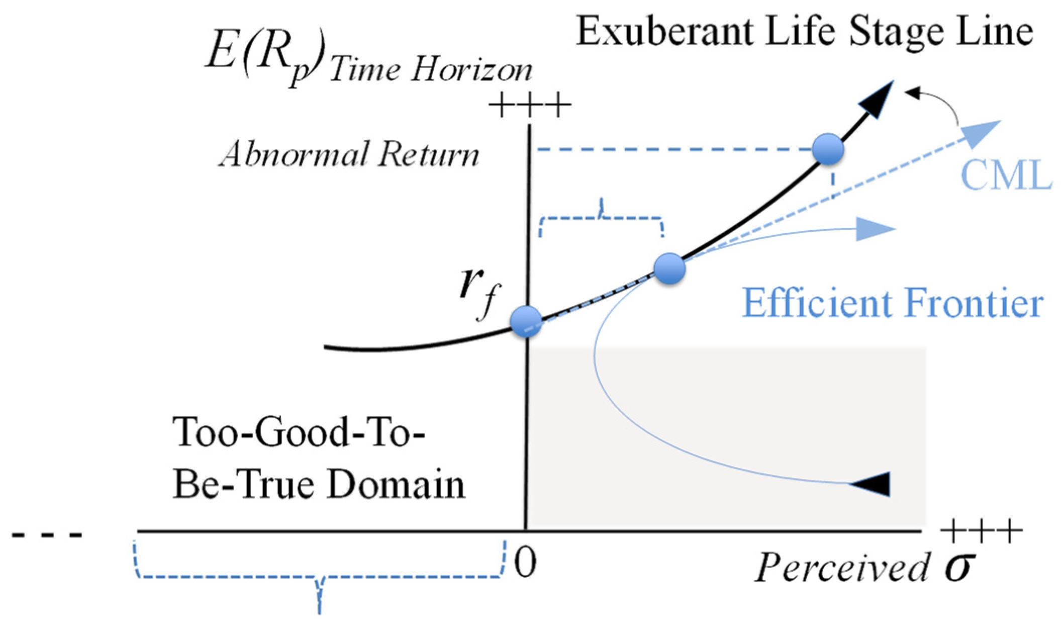
- The framework characterizes the type of construct (beginning, end constructs) and the types of bonds between the variables. We use only the “influence” bond out of the four main types that DPM recommends, in three of its forms: direct influence—positive (I+) or negative (I−)—and indirect—moderating (I±). In the framework presented in Figure 1, rf is the starting point and the “abnormal expected return” the end point;
- (2)
- Constructs are of the same nature. For this reason, we do not refer to risk but to perception of risk;
- (3)
- Symmetry of and among the constructs is of the essence and we assign an equal conceptual weight to each one, until proven otherwise;
- (4)
- Parallelism is paramount: for example, the mathematical functions we use are assumed to be quadratic. We develop our argument on that basis (parallelism outweighs standard assumptions supporting existing models). For this reason, we consider the Capital Market Line (CML) to be a portion of a larger quadratic function, even if this can be strongly debated (see further below). This is because in DPM, all constructs and all of their treatments are assumed upfront to be equal (parallel) until proven otherwise. This assumption is necessary because we are dealing with emerging concepts and do not yet know which constructs take precedence, to what level, and in what order (e.g., precedence, consequence). Hence, we need to keep all options open rather than arbitrarily deciding how to organize the constructs and their characteristics. In the present case, this is because we assume the efficient frontier to be in a quadratic form; by parallelism, we postulate that all other curves of a similar nature are also quadratic. This is not carved in stone; it is merely a technique that DPM suggests to set baselines by studying as yet “unidentified behavioral objects”, namely, emerging concepts;
- (5)
- A multidisciplinary approach allows the researcher to leave no stone unturned and discover “hidden truths”, especially in the context of emerging constructs. In the present case, multidisciplinarity is exposed in Table 1, which compares equivalent constructs across various disciplines. In DPM, these equivalences are considered as possible evidence of the validity of the emerging constructs under investigation.
These tenets require a meticulous approach in conceptual development and an open-mindedness that can be challenging.
2.3. The Other Tools
We set the EMH as the behavioral baseline, against which we compare the dysfunctional behavior of CFS. The former states that in highly efficient markets the investors: (1) have access to all relevant information immediately and at no cost; (2) have a primary goal of maximizing their wealth; (3) share the same risk and return projections; (4) trade financial assets for the same particular periods; and (5) weigh risk and return expectations. From a macroscopic perspective, market agents’ actions ultimately benefit societies, because the money earned will be reinvested to create jobs and new technologies. The exclusive pursuit of self-interest, for decades at the base of many economic theories, does not interfere with social welfare (Fehr and Schmidt 1999). The long-discussed, strongly criticized Rational Choice Theory (RCT), a somewhat marketing equivalent of EMH, adopts a similar posture: consumers are rational decision-makers facing preferential choices based on utility, and they have the computational ability and/or skills that enable them to maximize their expected gains (Bettman et al. 1998). We contrast EMH and RCT with the CFS framework and posit that spinning, while also based on selfish interests, obligatorily leads to market havoc. We enlarge the use of the CAPM by applying it to all kinds of assets, including those traded outside the stock markets (e.g., household/property assets), and add a spinning component to it. Recall that the original CAPM formula is as follows (Equation (1)):
E(Rp) = rf + β ⋅ [E(Rm) − rf]
For simplicity and breaking with the tradition, we rephrase as follows:
E(Rp) = rf + β ⋅ Ω
This formula assumes a linear relationship between the expected return on a portfolio E(Rp) and a single predictive factor—the market risk premium (Ω), which is expressed by the difference between the expected return of the market E(Rm) and the risk-free rate of return rf. This formula has been and still is widely used by financial experts and has been tested with mixed results over the decades (e.g., Black et al. 1972). Academics, including the original creators of this formula, have offered many variations of it noting, for example, that, “The CAPM is based on many unrealistic assumptions. For example, the assumption that investors care only about the mean and variance of one-period portfolio returns is extreme” (Fama and French 2004, p. 37). Many scholars have added one or more explanatory variables to the original, single linear regression (Equation (1)). For example, Fama and French (1996) proposed a three-factor model for expected returns, mostly in the context of how rapidly stock price responds to markets, and then a five-factor model (Fama and French 2015). The Consumption-Based CAPM (CCAPM) considers changes in the consumption index. These additions have not solved the impasse between the original rational and the irrational pricing viewpoints (mishaps in CAPM due to mispricing, partly resulting from biases, heuristics, and overreactions—De Bondt and Thaler 1985) in consideration of some empirical failures of the CAPM (Fama and French 2004, 2015). We also resort to what we call the Efficient function (illustrated in the Capital Frontier Theory—CFT), but do not limit it to a portfolio of financial assets traded, for example, by traders on the stock market. As indicated, we take the stand of average borrowers who have a regular portfolio of assets such as property, life insurance, bonds, stocks, and the like. We consider that what we refer to as the Efficient Frontier function is quadratic, in the horizontal form of x = f(y) = ay2 + by + c, where x is a function of y (admittedly, a debatable assumption). It makes sense that a positive, linear relationship exists between risk (measured by the standard deviation σ) and the (expected) returns E(Rp) on the portfolio p: buyers of speculative financial products expect to be better rewarded if they take on more risk when investing, and if they are rational there is no reason to believe that returns grow much faster than risk. As it is well known, when the CML (which represents a mean-variance efficient frontier for riskless assets) touches the EF function (which at that point represents a minimum variance frontier for risky assets), maximum benefits are secured; beyond that point and along the CML, consumers have to borrow money while incurring increasing risk. This means that the buyers of speculative financial products may become exceedingly aggressive as they are enthusiastically willing to borrow to materialize the expected portfolio return. Debt builds up, but the consumers of financial products are not spinning, they are merely acting as normal, rational investors who take calculated risks. What if, however, an awry tendency develops? The higher the debt, the more the consumers borrow to reach their elusive dreams, and the higher the debt, the more exuberant those dreams must be, because only by becoming wealthier to an exuberant degree can they reimburse their debt. What if, indeed, consumers start spinning and engage in such a wheel of misfortune?
3. Consumer Financial Spinning
In this section, we first define CFS more specifically, then illustrate it using the data percolation conceptual methodology.
3.1. Definition
In a booming, predatory economy where sales agents are actively engaged in push sales efforts, CFS refers to consumers of speculative financial products who disconnect from their initial hierarchy of needs (N), wealth-building goals (G), and preferences over the portfolio of their household assets (P) while engaging, knowingly or not, in a wheel of misfortune, much like a hamster stuck in a rotating cage. Over a short period of time of approximately 24 months (Kaminsky and Schmukler 2003), this rupture entails a significant reduction in both the consumers’ sensitivity to these NGPs and in their risk aversion, but a significant increase in levels of market stress (frictions), financial contagion, moral hazard (expressed by the dark financial triangle), and debt (Dow 2000). The wheel of misfortune is a debt trap for the market agents involved, and eventually for the entire market as contagion spreads, inevitably leading them to spin out of control and face a market crisis. In particular, their disconnection from original needs entails that the borrowers will never be satisfied, their disconnection from the initial goals indicates that the goals will remain elusive, and their disconnection from their initial preferences suggests a utility loss as they are likely to buy financial products that do not fit these preferences.
The predatory paradigm, which stands apart from equilibrium inherent to the economistic paradigm (e.g., EMH), is structurally formed of five constituents: it requires the active presence of seller-predators and customer-prey of financial products, one or more predatory tools (e.g., a predatory mortgage or predatory account the likes of those fostered by Wells Fargo in the 2000s in the US), some financial harm caused to the customer-prey, and a surprise effect (necessary to catch the prey off guard), such as a sudden, unexpected change in interest rates or a well-hidden contract clause. This is functionally expressed as follows: the cunning sellers identify their prey’s vulnerabilities; they bait them with attractive terms and mystifying promises (usually high returns); they put pressure on their prey to hasten decisions with as little valid information as possible; they trap the prey with, for example, contracts that serve their interest and that are built to confuse the prey and the regulatory authorities; and finally, they subdue their prey, for example with direct or indirect threats of foreclosures. We call this the 5–5 predatory net. Note that in Figure 1, because all the variables are psychological constructs, the scale is 0 to 100, not values found, for example, in the market (e.g., a beta β of 1.18). A risk aversion of zero means no risk aversion at all; one at 100% means that the borrowers would not engage in any purchase of speculative financial products at all. One hundred percent always represents the maximum value that the market agents are capable or willing to accept to stay within the CFS framework. This observation will be instrumental in Equations (4) and (5).
Predatory markets are characterized by claims of extraordinary (too-good-to-be-true) gains, heavy and deceitful advertising accompanied by marketing sweeteners (sweet deals), intensive push selling endeavors, reduced choices and horizons, as well as risk-hiding financial instruments and procedures. From the customer-prey’s point of view, spinning is the irrational expectation of high returns regardless of risks on a dangerously limited portfolio of assets while accumulating an unsustainable debt, in a short time horizon.
3.2. Some Key Definitions
Table 2, Table 3 and Table 4 give a summary based on a review of the literature of the key aspects of each of the three variables that have relevance in this article.
In summary, there is overwhelming evidence that market agents are not purely rational and do not behave with an immaculate sense of ethics. The three components of the DFT cover the standard elements that generally compose attitude in marketing: affective (overconfidence), cognitive (r-rationality), and conative (deceit). They parallel the three components of white-collar crime (organizational opportunity, financial motive, and deviant behavior—Sutherland (1924)) and the Dark Triad concept (Babiak 1995; Jakobwitz and Egan 2006) much acknowledged in studies on psychopathy, namely and respectively: narcissism, Machiavellianism, and deception. They are also in line with the fraud triangle framework: incentives and peer pressure (emotional), rationalization (intellectual), and opportunity (behavioral)—(Soltani 2013). On the right side of Figure 1, one can assess that sensitivity and risk aversion are both on a downward trend (↓). Hence, our proposed framework may offer a glimpse of dysfunctionality, as adapted to the financial context.
Under the EMH, there is no DFT, since agents are rational and asset prices reflect fundamental values (something deception, for example, could not allow); the CAPM formula expresses in some interpretative way at a maximum of only three constructs: sensitivity (≈β), risk (aversion (≈rf), and (exuberant) returns (≈[E(Rp]). The process embodied in the CAPM and conservative financial theory is purely cognitive; behavioral finance has complemented it with the notion of biases (which include overconfidence) and heuristics (which remain largely cognitive factors). Prospect theory has contested the utility theory, by which agents are said to gamble according to preferences determined by a set of mathematical axioms (completeness, continuity, independence, and transitivity)—(Von Neumann and Morgenstern 1947). It recognizes that people are risk averse over gains and risk seeking over losses. Additionally, people give more value to outcomes that are certain than to outcomes that are merely probable. In stark contrast, the CFS framework assumes that rationality and emotions are dependent on one another. This reflects the neurobiological system of market agents: a purely cognitive agent simply does not exist. All market agents have emotions, share thoughts, and manifest behaviors. Consumer financial spinning is not concerned with mathematical assumptions or axioms, or with comparisons between gains and losses or between outcomes. This is because when disconnected, consumers fail to process valuable information: they are intellectually numb, and rationally rationed. They do not get to the point where they can see the benefits of analyzing, comparing, evaluating, and weighing options. As for other advances made in behavioral finance, no research we know of has incorporated the DFT into the CAPM. A fair amount of effort has been made to express biases mathematically, but these remain to be empirically tested within the CAPM formula.
4. The Spinning Framework Using the CAPM-Markowitz Models
In this section, we free ourselves from the constraints of standard finance theory for the purpose of exploring a possible way of illustrating CFS. We do not pretend that the results hold true; rather, this is a conceptual exercise embedded in the regular dynamics of scholarly research. We go through several deployments of the spinning framework to explain its various parts. One should keep in mind that spinning being a process, all graphs are quintessentially under the pressure of a time horizon.
4.1. The CFS-Markowitz-Modified CAPM Framework
Our first step is to assume that dysfunctional consumers detach from the reasoned CML and form a line of their own, which we call the Exuberant Life Stage Line (ELSL), to use parallelism and hence assume that the latter is a portion of a larger vertical quadratic function, because we also consider that the efficient frontier is a quadratic function (a horizontal one). The ELSL has the format f(x) = ax2 + bx + c, where x = the standard deviation σ and the coordinate of the vertex of the horizontal axis of symmetry of the parabola, y = the expected return on the investment portfolio E(Rp), where a and b contract (large a and/or b) or widen (small a and/or b) the parabola and are >0 (if <0, then the parabola would deploy downward), and c moves the curve up or down along the Y-axis (Y-intercept)—Figure 1.
Note: Because the Exuberant Life Stage Line (ELSL) is assumed to be a parabola, it implies the use of the left quadrant, which we name the “too-good-to-be-true domain”. A time horizon is added to the Y-axis as this is where the borrowers (future buyers of high-stakes financial products) act: they change their expectations over their time horizon depending on perceived risk. The latter replaces σ, because under the principles of symmetry and parallelism, all constructs pertaining to the two market agents—lender and borrower—must be psychological in nature.
Figure 1 reads as follows (from left to right). The too-good-to-be-true domain is illusional: technically, there is no such thing as negative risk. To read it properly, one must think in psychological terms: to the right is the domain where the market imposes its conditions, hence the perceived risk. In the left domain, the consumer is led to think the market can be beaten. For a short while, between the risk-free rate rf and the point where the CML touches the Efficient Frontier, the ELSL espouses the regular CML as a quasi-straight line (both curves are reflective of the life stage of the customers: as income rises with advancement in career, they can borrow more and invest more). Note that the assumption that the ELSL is a parabolic function that tends to narrow means that its a and b increase overall. Note that the parabola and its extension into the left quadrant, which is an imaginary one, also represents reality. Many financial scams build on this too-good-to-be-true domain. Bernard Madoff and his immense Ponzi scheme provides a perfect example, among many others (Enron, Bre-X Minerals, Norbourg, etc.): his clients were led to believe he could systematically beat the market no matter how volatile it was, promising (abnormal) rates of return of some 15% year after year, without any interruption, regardless of economic conditions. Note also that risk σ is listed as perceived risk, as all constructs must be psychological in nature, and that time horizon has been added to the expected return variable E(Rp)time, because this system is predatory: time horizon is of the essence.
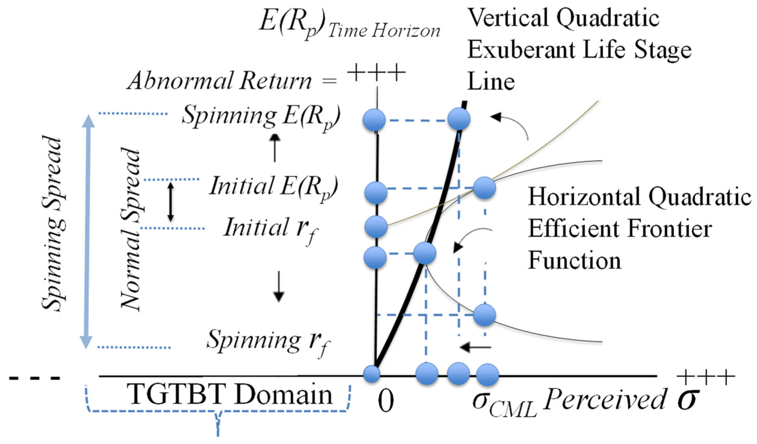
Our second step is to examine in more detail what happens to the various elements that are included in the framework (Figure 2).
Note: Because the ELSL is assumed to be a parabola, it implies the use of the left (unrealistic) quadrant; also, rf shifts down to spinning rf (valued at 0).
Figure 2 reads as follows (from left to right). We added wording in the too-good-to-be-true (irrational), “Madoff”, domain indicating that there are two vertical spreads: the normal one, and the spinning one, characterized by an inflated expected return E(Rp)’ of the portfolio and a deflated risk-free rate of return rf’. One can see that while the expected returns reach new highs (↑), the alleged risk-free rate diminishes to the point of absence of risk (→0). This is emblematic of predatory behaviors, just like promising a too-go-to-be-true outcome. All financial scammers try to convince their prey that their financial system is risk-free (otherwise, why would anyone venture to buy into it), or else they try to hide risk through incomprehensible contracts (or websites) and complex financial instruments. The widening, net effect of the spread between expected return and the risk-free rate is because ELSL replaces the CML for the greedy consumers as can be seen in the right quadrant. Financial predators bet on their prey’s risk aversion and offer them “heaven” by promising (abnormal) high returns and low risk, often claiming they have the ultimate, privileged (if not secret) recipe for success. The ELSL narrows when moving to the left, while the borrowers are traveling backward on the EF function, which is possible because their time horizon shrinks. While the expected return E(Rp) is boosted (↑E[Rp])’, the borrowers’ perceived risk is moving backward (←σ’), towards the point of origin (rf’ and σ = 0). Eventually, the borrowers will move to the right along the perceived risk X-axis (σ’→) as they become disconnected and because they follow what others do, and what others do is to take on more risks in a booming market. The net graphical result is that the market risk σm then moves right (σm→) and borrowers’ risk σ’ moves right as well, but always trailing the market (σ’ < σm).
Our third step is to incorporate the three components of the dark financial triangle in the spinning model. For the same level of risk (σ), the borrowers think they can beat the market and make themselves believe they can reach higher standards of living quasi instantly, like a lottery (abnormally high E[Rp]). This corresponds to overconfidence. We make this association because when overconfident, borrowers skip rungs along their ladder of needs. The idea behind this is that, as any financial advisor knows, people go through a certain hierarchy of financial needs as they engage more fully in the fabric of society, starting with saving accounts, life insurance, retirement savings, and then purchases of bonds and eventually, risky stocks. When overconfident, borrowers skip over some of the basics and invest blindly into high-risk products, as is the case in about every other financial crisis. R-rationality finds an expression by the fact that instead of satisfying themselves with a diversified portfolio, the borrowers focus all their attention on a very limited range of financial products (lower part of the EF curve)―(Mani et al. 2013). In the case of tulipomania in Holland in the 17th century, it was tulip bulbs; in the case of the GFC, it was houses. Thus, borrowers let go of their preferences and buy whatever single product is out there that they think will make them rich fast. R-rationality is hence associated with preferences. Deceit occurs when the borrowers erroneously think that they can earn more than what the market has to offer (abnormally high E[Rp]) while benefiting from a lower risk-free rate of return than the established rate (lower than normal rf); however, they are fooling themselves and others and let the predator-sellers mislead them too. The spinning spread tells the story of a lie that all scams rely upon: “Make money fast, there is no risk and the deal is much better than what is out there, believe you me!” Disconnection from needs is fostered by overconfidence (rendered by rung skipping), of preferences by r-rationality (betrayed by portfolio shrinking), and of goals by deceit (revealed by increased spreads), all without due consideration to risk. Our fourth step is to confirm that the ELSL is riskier than the normal MCL, despite what the shrewd predatory lender-sellers would have the borrower-customers believe. To affirm this, we resort to standard indifference curves, commonly found in finance theory: as these curves deploy, they are known to become riskier, so that in our framework, the upward curvature of the ELSL signifies higher risks. Again, this framework suggests that the borrowers will not take on more risk than the market: their σp’ will not surpass σm set by the market (at all times, σp’ < σm). The only way to increase σp’ is if the market first sees an increase in its σm. Thus, there has to be a contagion effect. As one of the borrowers follows the market and takes on more risk, so do numerous other borrowers who also compose the market: all borrowers caught in spinning imitate each other. This eventually leads them all to spin out of control.
4.2. CAPM Revisited
We have resorted to the tenets of the DPM and selected some observations from past research—such as data showing that the beta β tends to be higher than predicted by the standard CAPM formula and that markets display substantial volatility that cannot be explained using standard economic assumptions (Cochrane 2005). The CAPM formula assumes that there is no emotional involvement on the part of investors (it is thus a perfect instrument for financial analysts but an incomplete one for the “household” investors), and thus that transaction costs and taxes do not affect decisions (hence, they are considered null), and neither do contagion effects. In particular, CAPM is insensitive to budgetary considerations: the investors have no monetary concerns, they can borrow and invest infinite amounts, in subdivisible parcels if they wish, and the markets exhibit consistency. However, observations from the reality of markets call for a multi-factor approach to the CAPM formula (Nicholson and Snyder 2017), which would explore the risk contribution of influencers other than the ones treated. Beside the CCAPM and the three-factor model we discussed previously, the Arbitrage Pricing Theory (APT—Ross 1976) has been significant; it does not assume a fully efficient market. However, it rests on assumptions that clash with the conditions set for the spinning model, namely: (1) existence of perfect competition (so that there is no asymmetry of information and no predator–prey dynamics); (2) investors are rational; (3) investors immediately react to undervalued assets and sell them when relatively overvalued (in the case of spinning, recall that consumers of financial products have lost track of their initial goals, so that they do not necessarily engage in arbitrage). In summary, the original CAPM, CCAMP, and APT assume that the borrowers are and remain sensitive to their initial needs, goals, and preferences, behave rationally and ethically, and that the market is safe and sound (economistic paradigm). All three assumptions go against the description of a predatory paradigm where CFS is likely to surface. Behavioral finance has expressed limitations over arbitrage and emphasized the recourse to psychology (Barberis and Thaler 2002), but it does not treat disconnection from reality, even though this is a phenomenon well studied in that field in its more technical term of disassociation.
Since we worked based on the assumption that all curves are quadratic, we temporarily reformulate the CAPM into a bi-explanatory-factor function, as follows:
E(Rp)’ = rf’ + β⋅Ω2 + ψ⋅Ω
The square of the market risk premium (Ω2) allows us to turn the original CAPM formula into a quadratic function. The added variable (ψ⋅Ω) acts as an amplification mechanism (Brunnermeier and Oehmke 2012) that betrays excessive speculation and, assuming that beta β and psi ψ do not differ wildly from another, has theoretically less impact on the expected return on the portfolio with respect to the market risk premium than the first variable (β⋅Ω2), which by essence was conceived in the context of purely rational investors. Psi (ψ), being parallel to beta β, must therefore measure sensitivity. Because spinning occurs in the context of indebtedness, and because we assume emotionality is related to money matters (people fear missing out on the opportunity to enter a booming market—where total income is increasing, but fear the risk of getting caught in a crashing market—where an unsustainable debt looms), we consider that the added variable (ψ⋅Ω) is a measure of emotionality in the context of spinning and propose to measure psi ψ as follows:
We view psi (ψ) as the expression of some of the assumptions made in behavioral finance: it discloses the impact that emotions, resulting from the fear of the debt trap, can have on decision-making (on choosing the illusory, abnormal E[Rp]’). At 100%, the fear is the most “household” investors can endure; at zero, there would be no fear at all (the marketers of risky financial products have done a great convincing job). Equation (4) does not tell the whole story, however. Recall that the predator-sellers are trying to move the prey-customers into the “Madoff” domain. To do this, they have to make extravagant promises (expressed by a boosted E[Rp] → E[Rp]’) while making customers believe that the risk-free rate of return is close to nil ( → 0). Hence, they have to maximize the spread between the two variables E(Rp)’ and . We finalize our spinning function as follows:
with rf > ≥ 0 and lim → 0. By dividing the market risk premium Ω by the risk-free rate of return rf, which in the context of spinning tends toward zero (→0), we express the fact that the inherent dynamic of the entire system is inflationary: predator-sellers sell a wild dream and buyer-prey buy into it. Recall that since we are dealing with psychological constructs, all scales are from 0 to 100, as previously indicated. In case of Equation (4), rf and are valued at 1, meaning that this equation reflects the most the “household” investors are willing or capable of conceiving: at that point, it would not be worth investing at all, because no spread would be achievable between the market rf and the spinning rf, as it is this spread that, in part, feeds the wealth appetite of these investors.
Equation (5) highlights the fact that the expectations of return on a portfolio (necessarily little diversified in the context of spinning) are artificially boosted (irrational) and that decisions are based on both cognitive and emotional considerations (expressed by debt). At beta β > 1, the portfolio is more volatile than the market; at 1, it matches the market; at 0, it is often interpreted as a cash market; at < 0, it is a counter-market, with gold often being a sample case of this occurrence. At psi ψ > 1, the borrowers may change opinion often. Looking at the interaction between beta β and psi ψ, one can derive that it might help to anticipate systemic risk (risks that pertain to the financial system but that are not necessarily systematic, that is, whose occurrence is not de facto predictable)1 and that are at the heart of financial crises (De Bandt and Hartmann 2000). Systemic risks include phenomena like bank runs, contagion, and liquidity crushes (Benoît et al. 2015). When both beta β and psi ψ are high, this points to market and individual volatility, and substantial unpredictability. This will inflate the irrational (abnormal) expected returns E(Rp)’, which call for aggressive borrowing (greed). It is probably in that combination that the debt trap is the most treacherous. Note that because psi ψ is measured by two types of account—the ins (revenues) and the outs (debt)—it is very sensitive to such things as fees, taxes, income tax, black market revenues, and so forth. It is therefore much better positioned to reflect the reality of the market than the original CAPM formula. This signifies that consumers, before disengaging from their initial financial needs, goals, and preferences, work hard not only to maximize the positive outlooks—E(Rp)’ and total income, but also to minimize whatever jeopardizes them—fees, taxes, and so forth. In short, it is to their best selfish advantage to cheat the system, as long as the risks of being caught remain inconsequential. This is truly a predatory paradigm. This also holds true for unscrupulous lenders, as they will benefit handsomely from spinning clients who spend without counting.
Equation (5) may permit portfolio managers to evaluate their clients’ desired returns, based not only on the assumption that they are rational, as should be the case, but also that they may be irrational at times (see Appendix A). It offers a way of measuring the potential for irrationality based in part on known variables—income and debt; we are not arguing here that Equation (5) gauges irrationality for certain. For this proposed equation to make sense in the market, it should be tested on a vast number of consumers of financial products to set its baseline. At what level does psi ψ become irrational? The advantage of Equation (5) is that it calls for hard data rather than for subjective assessments of irrationality or the DFT. It is highly contextualized because it relies on the spinning rf, which is an abnormal occurrence. We suppose that many studies will be necessary in the future to come up with a table of acceptable levels of psi ψ given rf’. However, in the meantime, and as part of an exploratory effort, we can determine whether the ELSL may indeed curve upwards, away from the CPL, and under what conditions. This is what we discuss in the next section, which details the research we conducted, keeping in mind again that the measuring tools for CFS are still being developed and that our effort tackles an emerging concept.
5. Exploratory Field Study and Results
For obvious reasons, we could not test the entire framework we propose. Even if we could, it would require several articles to go through the results. Also, as mentioned, the risk-free rate of return is only rarely perceived as being below the offical rate. During the GFC, for example, the beneficiaries of teaser rates viewed them as risk-free rates below the official ones. They likely felt justified to enjoy a better rate than those who chose non-predatory, conventional mortgages. Occasions when the perception of a risk-free rate that approximates zero are often the fact of scams: sales agents (for example, a Ponzi scheme) claim there are no risks, and incidentally, that the networks they establish are reserved for the privileged, and hence must be kept secret. Rather than wait for the next crisis to develop or try to enter into a scam network, we decided to test one part of the model: the assumption that the ELSL may curve upwards instead of following the rational, linear CML trend. It must be noted again that we are not contesting the linearity involved in the CML; we are rather saying that in a predatory paradigm, irrationality may build up to a point where the behaviors of the consumers of financial products derail (DeLiema et al. 2020). What we want to check is whether or not we can find a combination of factors that cause such derailment, that is, that cause disconnection from the initial NGPs. Put simply, we want to define more accurately the wheel of misfortune.
Because at the present time there is no established questionnaire to measure CFS, and as this is a new, emerging concept, we created a questionnaire based on an established questionnaire that has served in numerous studies on predator/seller–prey/buyer interactions (Mesly 2010). We added questions that we felt could measure the variables of interest (VOIs). If anything, it could serve as a base to develop a full-fledged questionnaire in the future. With these constraints in mind, we had our questionnaire distributed electronically to hundreds of small-time investors who were clients of a network of financial advisers with whom we were and still are acquainted. The questionnaire appears in Appendix B; we added various questions to hide the true nature of the questionnaire so as not to bias the respondents’ participation. This is a common technique employed in psychological testing (Mesly 2015). In the section that follows, we focus only on the main results to illustrate that our proposed framework could make sense under certain conditions, keeping in mind that we take a psychological approach as opposed to large databases commonly used in econometrics.
Results
We received 221 responses, of which 195 were deemed valid, accounting for 48.5% female and 51.5% male. We divided the results into two parts: one running linear regressions using SPSS 25 and the other exploring a structural equation model (SEM) using Amos, part of the same IBM statistical software.
The key significant linear regression appears in Table 5.
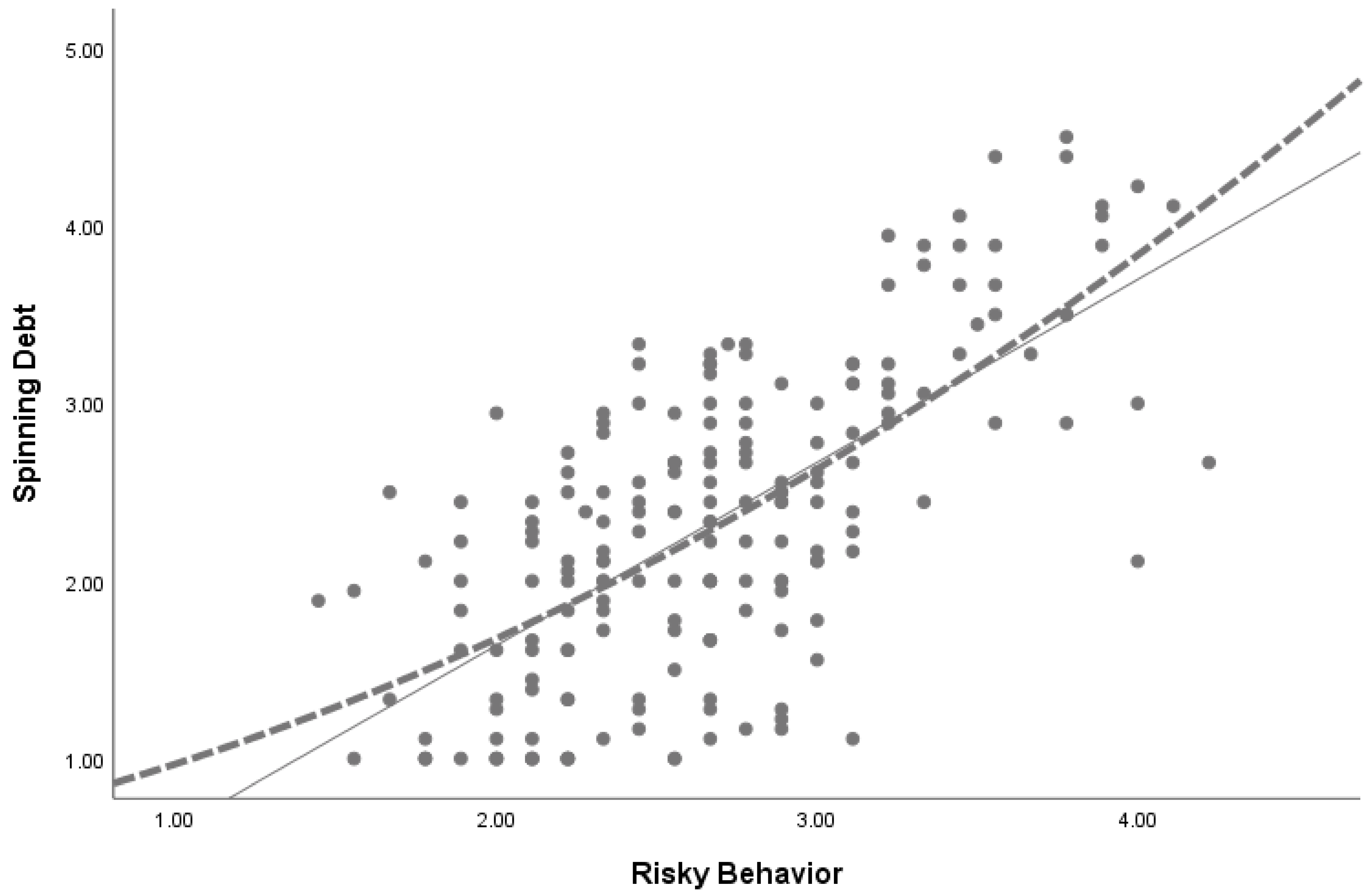
Nearly 46% of the variance in what we define as a spinning debt (calculated as the average of debt + exuberant + unsustainable) is explained by risky behavior (calculated as the average of speculative behaviors + poorly diversified portfolio + short-term horizon). The relationship is linear and significant at 0.000. This presumes that each component of each VOI is independent and has equal weight. This result is in line with standard financial theory. However, note that we can also fit in a quadratic function, which achieves an R2 of 0.461, minimally above the R2 of 0.458 in the linear regression.
Figure 3 compares the two approaches. The quadratic function presents a noteworthy difference: the curve starts at 1:1, which is the point of origin on the 5-point Likert scale used. This point can be interpreted as the anchor (beginning) point; it depicts a more realistic picture than the linear function, which, when extrapolated towards the Y-axis, leads to a negative expected return (expressed as spinning debt in the model).
Note: The linear function between spinning debt (expected returns fed by debt) and risky behavior contrasts with the proposed quadratic function, which starts at the point of origin.
This result can by no means be interpreted as proof of a quadratic tendency of the CML, but it is enough to justify further studies, once the questionnaire is perfected. Recall that our questionnaire was distributed in normal market conditions; it may be possible that in predatory conditions, debt, exuberance, and unsustainability affect each other symbiotically (each component would then be multiplied by the other). In that case, and assuming the same definition of risky behavior, the curvature then becomes even more pronounced, reaching an R2 of 0.515. Such a scenario would likely occur when consumers push their level of irrationality and become nervous about the market: debt encourages a greater need for achieving higher returns, but then becomes even more intolerable, and so forth. We assume that this would characterize a wheel of misfortune.
The empirical implications are that, if it were true that irrationality may bend the CML, fund managers would have a keen interest in understanding not only their clients’ level of risk aversion when investing their funds, but also their level of CFS, real or potential. More precisely, tools could be developed to assess how disconnected clients are from their NGPs, which could be an indicator of bad investments to come.
6. Conclusions
In this article, we suggested that relaxing and reframing some of the basics of standard financial theory within the realm of consumers acting in toxic financial environments draws a realistic picture of their harmful, consequential spinning. We defined what the wheel of misfortune must entail to justify a curved Exuberant Life Stage Line, an adapation of the Capital Market Line to correspond to unique, predatory market conditions.
We aimed to initiate the development of a theory for the emerging concept of CFS that has far-reaching financial, legal, and marketing consequences. We used the analogy of the hamster spinning its wheel (of misfortune), combined previously unconnected bodies of knowledge (finance, marketing, and psychology), invoked several existing theories and methods, and endeavored to raise the comprehension of CFS to another level. We proposed a graphical and parsimonious mathematical rendition of that phenomenon. The data percolation methodology helped us identify the key constructs and their operational links.
Our approach is unorthodox and wide open to severe criticism, but this is precisely the role of conceptual development; it will generate heated debate and may entice research, which is how science evolves. Our innovative use of financial tools and a unique consumer behavior perspective allowed us to offer an explanation as to why market agents get caught in Ponzi schemes the likes of Madoff’s. We showed that we could render the DFT using portfolio, risk, and spread parameters. We also proposed that if market conditions heat up to a certain level, debt must be compensated with higher expected returns and implies more debt, which, as it becomes increasingly unbearable, leads to more desperate borrowing, engaging the customers into a wheel of misfortune bound to cause financial distress.
Our framework, while insightful, is far from complete. We did not include personality (as a psychological construct), although some personalities are more geared toward risk taking than others. Future research will likely examine the proposed framework’s potential for predicting consumers’ indebtedness patterns, and could venture into examining whether or not it applies to contrasting economies. Developing some metrics, as has been done for the beta β of the CAPM formula over the decades, could affirm or disprove the robustness of the CFS framework. The framework contains additional limits: it may be that psi ψ cannot be fully measured by the notions of total debt and total income—however, as income fails to cover debt, panic may kick in and recourse to morally hazardous behaviors may feel like the only way out.
In this article, it was sufficient to propose an original, multidisciplinary view of the emerging concept of CFS, given that is it an idiosyncratic consumer behavior entrenched in exceptional, flawed market conditions hardly explored to date. We believe that this holds potential for theory, but also for the marketplace. Borrowers who acquire high-stakes, intangible, and complex financial assets in a “culture of vulture” market are vulnerable, even more so as often their life savings and lifestyle are on the line.
The implication for financial practitioners is that one must be cautious when allowing easy access to credit or engaging in risk maneuvering, for example by way of securitization as was the case during the GFC. Sellers of financial products could run a reality check with their clients to ensure that no CFS is building up, either as a psychological undertow or out in the open. Future research could also investigate the possibility of creating a CFS-centered self-assessment test, for example. Another avenue would be for managers to run seminars to guide their clients and sensitize them to the possibilities of CFS, especially in predatory markets. Our study also hints at the need for better regulations to protect overly speculative consumers and for improving regulators’ understanding of how unscrupulous lenders can go about abusing and destabilizing markets. Certainly, in our opinion, there are legal implications in fostering CFS and driving the economy on a downward path that benefits only a few but harms many.
Funding
This research received no external funding.
Institutional Review Board Statement
Ethical review and approval were waived for this study, because the research was deemed to meet the minimal risk criteria set by the guidelines of the Declaration of Helsinki.
Informed Consent Statement
Informed consent was obtained from all subjects involved in the study, with full contact information of the researcher provided.
Data Availability Statement
The data is locked stored at the researcher’s academic institution office and will be kept for five years from date of collection.
Acknowledgments
The author wishes to thank the following professors for their input: Sabri Broubaker, Nicolas Huck, Luc Meunier, Hareesh Mavoori, Duc Nguyen, Françcois-Éric Racicot, and David Shanafelt.
Conflicts of Interest
The author declares no conflict of interest.
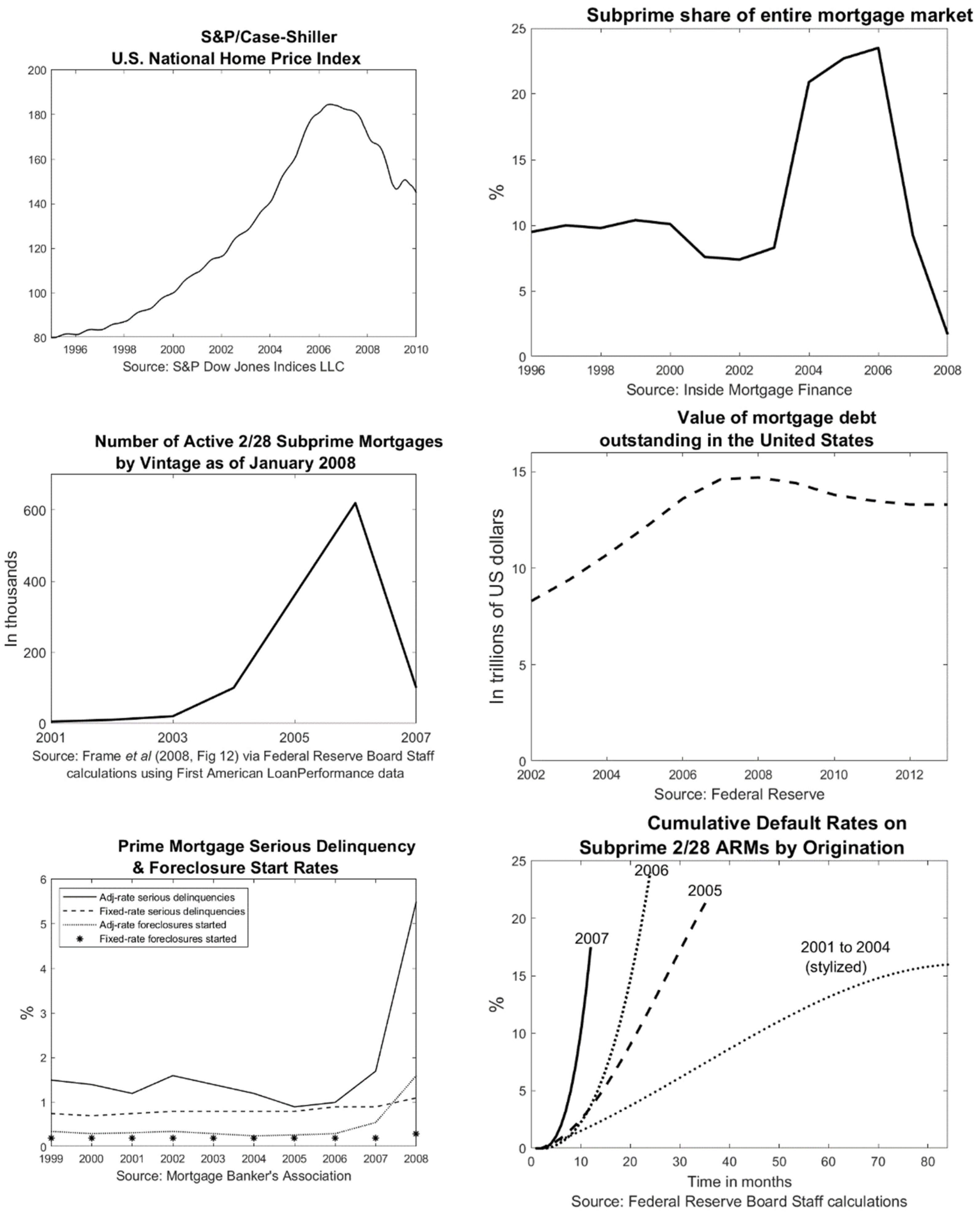
Appendix A. Proposed Evidence of CFS during the Global Financial Crisis
Figure A1.
Proposed Evidence of CFS During the US GFC. Note: The above graphs may tell the story of CFS and of pay now and pay (dearly) later.
Figure A1.
Proposed Evidence of CFS During the US GFC. Note: The above graphs may tell the story of CFS and of pay now and pay (dearly) later.

As can be seen from the left-hand graph on the first row (R1-LG), house prices in the US peaked in 2006. During the period leading to that peak, borrowers relied increasingly on the risky adjustable-rate and predatory mortgages, which were vulnerable to interest rates once the teaser period had passed (R1, right graph RG, and R2-LG). Debt kept increasing and remained high after those peaks (R2-RG), and, starting in 2007, foreclosures exploded (R3-LG). The bottom right-hand graph R3-RG shows how the tragedy accelerated, especially from 2005 to 2007. People frantically bought houses and properties seeing them as investment opportunities, as if there were no risk involved, but the situation soon spun out of control.
Appendix B. Excerpts from the Embryonic Questionnaire

| Spinning Debt Latent Variable |
| Debt |
| I very often borrow beyond my means. |
| I tend to be late in paying my debts. |
| I owe a lot of money. |
| Unsustainable |
| I have large debts compared to my capacity to reimburse them. |
| My total income is not enough to cover my total debt. |
| I am unlikely to be able to reimburse all my debts any time soon. |
| Exuberance |
| Despite having to borrow, I cannot resist an investment opportunity. |
| Risky Behavior Latent Variable |
| Speculation |
| I tend to invest with little regard to risk. |
| I like to gamble without paying much attention to my realistic chances of winning. |
| I do not like to take financial risks. (reverse). |
| Narrow |
| I only invest in a narrow range of financial products. |
| I am happy investing in one or very few assets like a house or bonds. |
| I do not have a well-diversified portfolio of financial assets. |
| Horizon |
| When I invest, I look for short-term gains. |
| I expect to earn money quickly when I invest. |
| I am in the financial market for the long run (reverse). |
| Disconnection Latent Variable |
| From Need |
| I am attuned to my financial needs (reverse). |
| I have carefully identified my financial needs (reverse). |
| I understand my financial needs (reverse). |
| From Goal |
| I have identified my financial goals with great care (reverse). |
| I have set my financial goals (reverse). |
| I stick to the financial goals I set (reverse). |
| From Preferences |
| I have determined which financial products I prefer (reverse). |
| I know which attributes I like and do not like in financial products (reverse). |
| I know what I do and do not like about the financial products in which I invest (reverse). |
| Sociodemographics |
Note: This is an exerpt from our questionnaire aimed at measuring key VOIs pertaining to the phenomenon of CFS. We only show the results that we deem significant to the framework we presented. We found no linear relationships between disconnection from NGPS and spinning debt or risky behavior.
| 1 | According to the European Central Bank (2010) systemic risk is a risk “so widespread that it impairs the functioning of a financial system to the point where economic growth and welfare suffer materially”. Accessed 1 September 2021. |
References
- Babiak, Paul. 1995. When psychopaths go to work. Applied Psychology 44: 171–88. [Google Scholar] [CrossRef]
- Baker, Malcolm, and Jeffrey Wurgler. 2007. Investor sentiment in the stock market. Journal of Economic Perspectives 21: 129–51. [Google Scholar] [CrossRef] [Green Version]
- Barberis, Nicholas, and Richard Thaler. 2002. A Survey of Behavioral Finance National Bureau of Economic Research NBER Working Paper No. 9222. Available online: https://www.nber.org/papers/w9222 (accessed on 2 June 2021).
- Benoît, Sylvain, Jean-Edouard Colliard, Christophe Hurlin, and Christophe Pérignon. 2015. Where the Risks Lie: A Survey on Systemic Risk. HEC Paris Research Paper No. FIN-2015–1088. Available online: https://papers.ssrn.com/sol3/papers.cfm?abstract_id=2577961 (accessed on 23 July 2021).
- Bettman, James R., Mary Frances Luce, and John W. Payne. 1998. Constructive Consumer Choice Processes. Journal of Consumer Research 25: 87–217. [Google Scholar]
- Black, Fischer, Michael C. Jensen, and Myron Scholes. 1972. The Capital Asset Pricing Model: Some Empirical Tests. In @Studies in the Theory of Capital Markets@. Edited by Michael C. Jensen. New York: Praeger, pp. 79–121. [Google Scholar]
- Boush, David M., Marian Friestad, and Peter Wright. 2015. Deception in the Marketplace: The Psychology of Deceptive Persuasion and Consumer Self-Protection. London: Routledge. [Google Scholar]
- Brunnermeier, Markus K., and Martin Oehmke. 2012. Bubbles, Financial Crises, and Systemic Risk NBER Working Paper No. 18398. Available online: https://www.nber.org/papers/w18398 (accessed on 30 May 2020).
- Campbell, John Y., Andrew W. Lo, and A. Craig McKinlay. 1997. The Econometrics of Financial Markets. Princeton: Princeton University Press. [Google Scholar]
- Chakravarti, Ashok. 2017. Imperfect Information and Opportunism. Journal of Economic Issues 51: 1114–36. [Google Scholar] [CrossRef]
- Cleeren, Kathleen, Harald van Heerde, and Mamik G. Dekimpe. 2013. Rising from the ashes: How brands and categories can overcome product-harm crises. Journal of Marketing 77: 58–77. [Google Scholar] [CrossRef]
- Cochrane, John H. 2005. Asset Pricing. revised ed. Princeton: Princeton University Press. [Google Scholar]
- Copes, Heith, and Lynne M. Vieraitis. 2012. Identity Thieves: Motives and Methods. Boston: Northeastern University Press. [Google Scholar]
- Coulibaly, Brahima, and Geng Li. 2009. Choice of mortgage contracts: Evidence from the survey of consumer finances. Real Estate Economics 37: 659–73. [Google Scholar] [CrossRef] [Green Version]
- Cowley, Elizabeth, and Christina I. Anthony. 2005. Consumers tell many lies. Deception Memory: When Will Consumers Remember Their Lies? Journal of Consumer Research 46: 180–99. [Google Scholar] [CrossRef]
- Daunt, Kate L., and Lloyd C. Harris. 2012. Exploring the forms of dysfunctional customer behaviour: A study of differences in servicescape and customer disaffection with service. Journal of Marketing Management 28: 129–53. [Google Scholar] [CrossRef]
- De Bandt, Olivier, and Philipp Hartmann. 2000. Systemic Risk: A Survey. ECB Working Paper, No. 35. Frankfurt: European Central Bank (ECB). Available online: https://www.ecb.europa.eu/pub/pdf/scpwps/ecbwp035.pdf (accessed on 5 June 2021).
- De Bondt, Werner F. M., and Richard H. Thaler. 1995. Does the stock market overreact? Journal of Finance 40: 793–805. [Google Scholar] [CrossRef]
- DeLiema, Marguerite, Doug Shadel, and Karla Pak. 2020. Profiling Victims of Investment Fraud: Mindsets and Risky Behaviors. Journal of Consumer Research 46: 904–14. [Google Scholar] [CrossRef]
- DePaulo, Bella M., Deborah Kashy, Susan E. Kirkendol, Melissa M. Wyer, and Jennifer A. Epstein. 1996. Lying in everyday life. Journal of Personality and Social Psychology 70: 979–95. [Google Scholar] [CrossRef] [PubMed]
- Dinica, Irina, and Damian Motteau. 2012. The Market of the Bottom of the Pyramid: Impact on the Marketing-Mix of Companies. Master’s Thesis, Umea School of Business, Umea Univeritet, Umeå, Sweden. [Google Scholar]
- Dow, James. 2000. What Is Systemic Risk? Moral Hazard, Initial Shocks, and Propagation. Monetary and Economic Studies 18: 1–24. [Google Scholar]
- Estelami, Hooman. 2015. Cognitive catalysts for distrust in financial services markets: An integrative review. Journal of Financial Services Marketing 20: 246–57. [Google Scholar] [CrossRef]
- Etkin, Jordan, and Anastasiya Ghosh. 2018. When being in a positive mood increases choice deferral. Journal of Consumer Research 45: 208–25. [Google Scholar] [CrossRef]
- European Central Bank (ECB). 2010. Financial networks and financial stability. Financial Stability Review, 155–60. [Google Scholar]
- Fama, Eugene F. 1970. Efficient Capital Markets: A Review of Theory and Empirical Work. Journal of Finance 25: 383–417. [Google Scholar] [CrossRef]
- Fama, Eugene F., and Kenneth R. French. 1996. Multifactor Explanations of Asset Pricing Anomalies. The Journal of Finance 51: 55–84. [Google Scholar] [CrossRef]
- Fama, Eugene F., and Kenneth R. French. 2004. The Capital Asset Pricing Model: Theory and Evidence. Journal of Economic Perspectives 18: 325–46. [Google Scholar] [CrossRef] [Green Version]
- Fama, Eugene F., and Kenneth R. French. 2015. A five-factor asset pricing model. Journal of Financial Economics 116: 1–22. [Google Scholar] [CrossRef] [Green Version]
- Fehr, Esrnst, and Klaus Schmidt. 1999. A theory of fairness, competition, and cooperation. The Quarterly Journal of Economics 114: 817–68. [Google Scholar] [CrossRef]
- Fenton-O’Creevy, Mark, Nigel Nicholson, Emma Soane, and Paul Willman. 2003. Trading on illusions: Unrealistic perceptions of control and trading performance. Journal of Occupational and Organizational Psychology 76: 53–68. [Google Scholar] [CrossRef]
- Fernbach, Philip, Chrsitina Kan, and John G. Lynch Jr. 2015. Squeezed: Coping with constraint through efficiency and prioritization. Journal of Consumer Research 41: 1204–27. [Google Scholar] [CrossRef]
- Gervais, Simon, and Terrance Odean. 2001. Learning to be overconfident. The Review of Financial Studies 14: 1–27. [Google Scholar] [CrossRef]
- Gilbride, Timothy J., and Greg M. Allenby. 2004. A choice model with conjunctive, disjunctive, and compensatory screening rules. Marketing Science 23: 391–406. [Google Scholar] [CrossRef]
- Griffin, Dale, and Lyle Brenner. 2004. Perspectives on probability judgment calibration. In Blackwell Handbook of Judgment and Decision Making. Edited by Derek J. Koehler and Nigel Harvey. Hoboken, NJ: Wiley-Blackwell, pp. 177–99. [Google Scholar]
- Griffin, Dale, and Amos Tversky. 1992. The weighing of evidence and the determinants of confidence. Cognitive Psychology 24: 411–35. [Google Scholar] [CrossRef]
- Grinblatt, Mark, Matti Keloharju, and Juhani T. Linnainmaa. 2012. IQ, trading behavior, and performance. Journal of Financial Economics 104: 339–62. [Google Scholar] [CrossRef]
- Harris, Lloyd C., and Kate L. Reynolds. 2004. Jay customer behavior: An exploration of types and motives in the hospitality industry. Journal of Services Marketing 18: 339–57. [Google Scholar] [CrossRef]
- Hoch, Stephen J., and George F. Loewenstein. 1991. Time-inconsistent Preferences and Consumer Self-Control. Journal of Consumer Research 17: 492–507. [Google Scholar] [CrossRef] [Green Version]
- Huang, Laura, and Jone L. Pearce. 2015. Managing the unknowable: The effectiveness of early-stage investor gut feel in entrepreneurial investment decisions. Administrative Science Quarterly 60: 634–70. [Google Scholar] [CrossRef] [Green Version]
- Huang, Shiao Yan, Chi-Chen Lin, An-An Chiu, and David C. Yen. 2017. Fraud detection using fraud triangle risk factors. Information Systems Frontiers 19: 1343–56. [Google Scholar] [CrossRef]
- Isen, Alice M., and John M. Reeve. 2005. The influence of positive affect on intrinsic and extrinsic motivation: Facilitating enjoyment of play, responsible work behavior, and self-control. Motivation and Emotion 29: 295–323. [Google Scholar] [CrossRef]
- Jakobwitz, Sharon, and Vincent Egan. 2006. The dark triad and normal personality traits. Personality and Individual Differences 40: 331–39. [Google Scholar] [CrossRef]
- Kahneman, David, and Amos Tversky. 1979. Prospect Theory: An analysis of decision under risk. Econometrica 47: 263–92. [Google Scholar] [CrossRef] [Green Version]
- Kaminsky, Graciela L., and Sergio L. Schmukler. 2003. Short-Run Pain, long-Run Gain: The Effects of Financial Liberalization. National Bureau of Economic Research NBER WP-9787. Available online: http://www.nber.org/papers/w9787 (accessed on 13 July 2021).
- Karlsson, Niklas, George Loewenstein, and Duane Seppi. 2009. The ostrich effect: Selective attention to information. Journal of Risk and Uncertainty 38: 95–115. [Google Scholar] [CrossRef]
- Laran, Juliano. 2010. The influence of information processing goal pursuit on post-decision affect and behavioral intentions. Journal of Personality and Social Psychology 98: 16–28. [Google Scholar] [CrossRef] [Green Version]
- Lavoie, Marc. 2004. Post Keynesian consumer theory: Potential synergies with consumer research and economic psychology. Journal of Economic Psychology 25: 639–49. [Google Scholar] [CrossRef]
- Lesch, William, and Bruce Byars. 2008. Consumer insurance fraud in the US property-casualty industry Consumer insurance fraud. Journal of Financial Crime 15: 411–31. [Google Scholar] [CrossRef]
- Lintner, John. 1965. The Valuation of Risk Assets and the Selection of Risky Investments in Stock Portfolios and Capital Budgets. Review of Economics and Statistics 47: 13–37. [Google Scholar] [CrossRef]
- Loewenstein, Groege F., Elke U. Weber, Christopher K. Hsee, and Ned Welch. 2001. Risk as feelings. Psychological Bulletin 127: 267–86. [Google Scholar] [CrossRef]
- Lusardi, Annamaria, and Olivia S. Mitchelli. 2007. Financial literacy and retirement preparedness: Evidence and implications for financial education. Business Economics 42: 35–44. [Google Scholar] [CrossRef] [Green Version]
- Lusardi, Annamaria, and Olivia S. Mitchelli. 2014. The economic importance of financial literacy: Theory and evidence. Journal of Economic Literature 52: 5–44. [Google Scholar] [CrossRef] [Green Version]
- Mani, Anandi, Sendhil Mullainathan, Eldar Shafir, and Jiaying Zhao. 2013. Poverty impedes cognitive function. Science 341: 976–80. [Google Scholar] [CrossRef] [Green Version]
- Manjit, S. Yadav. 2010. The Decline of Conceptual Articles and Implications for Knowledge Development. Journal of Marketing 74: 1–19. [Google Scholar]
- Markowitz, Harry. 1952. Portfolio Selection. Journal of Finance 7: 77–99. [Google Scholar]
- Mayer, Don, Anita Cava, and Catharine Baird. 2014. Crime and Punishment (or the Lack Thereof) for Financial Fraud in the Subprime Mortgage Meltdown: Reasons and Remedies for Legal and Ethical Lapses. American Business and Law Journal 51: 515–97. [Google Scholar] [CrossRef]
- Mehta, Nitin, Surendra Rajiv, and Kannan Srinivasan. 2004. Role of forgetting in memory-based choice decisions: A structural model. Quantitative Marketing and Economics 2: 107–40. [Google Scholar] [CrossRef]
- Mesly, Olivier. 2010. Voyage au Cœur de la Prédation Entre Vendeurs et Acheteurs—Une Nouvelle Théorie en Vente et Marketing. Sherbrooke: Université de Sherbrooke. [Google Scholar]
- Mesly, Olivier. 2015. Creating Models in Psychological Research. New York: Springer International Publishing. [Google Scholar]
- Mesly, Olivier. 2020. Spinning: Zooming in an atypical consumer behavior. Journal of MacroMarketing 41: 232–50. [Google Scholar] [CrossRef]
- Moore, Don A., and Paul J. Healy. 2008. The trouble with overconfidence. Psychological Review 115: 502–17. [Google Scholar] [CrossRef] [Green Version]
- Netemeyer, Richard G., Dee Warmath, Daniel Fernandes, and John G. Lynch Jr. 2018. How am I doing? Perceived financial well-being, its potential antecedents, and its relation to overall well-being. Journal of Consumer Research 45: 68–89. [Google Scholar] [CrossRef]
- Nicholson, Walter, and Christopher Snyder. 2017. Microeconomic Theory: Basic Principles and Extensions, 12th ed. Boston: Cengage Learning. [Google Scholar]
- Odean, Terrance. 1998. Do investors trade too much? American Economic Review 89: 1279–98. [Google Scholar] [CrossRef]
- Pyone, Jin Seok, and Alice M. Isen. 2011. Positive affect, intertemporal choice, and levels of thinking: Increasing consumers’ willingness to wait. Journal of Marketing Research 48: 532–43. [Google Scholar] [CrossRef] [Green Version]
- Ross, Stephen A. 1976. The Arbitrage Pricing Theory of Capital Asset Pricing. Journal of Economic Theory 13: 341–60. [Google Scholar] [CrossRef]
- Shah, Anuj K., Sendhil Mullainathan, and Eldar Shafir. 2012. Some consequences of having too little. Science 338: 682–85. [Google Scholar] [CrossRef] [PubMed] [Green Version]
- Sharpe, William F. 1964. Capital Asset Prices: A Theory of Market Equilibrium under Conditions of Risk. Journal of Finance 19: 425–42. [Google Scholar]
- Soltani, Baham. 2013. The Anatomy of Corporate Fraud: A Comparative Analysis of High Profile American and European Corporate Scandals. Journal of Business Ethics 120: 251–74. [Google Scholar] [CrossRef]
- Stüttgen, Peter, Peter Boatwright, and Robert T. Monroe. 2012. A satisficing choice model. Marketing Science 31: 878–99. [Google Scholar] [CrossRef] [Green Version]
- Sutherland, Edwin H. 1924. Principles of Criminology. Chicago: University of Chicago Press. [Google Scholar]
- Titus, Ricard M., Fred Heinzelmann, and John M. Boyle. 1995. Victimization of Persons by Fraud. Crime and Delinquency 41: 54–72. [Google Scholar] [CrossRef]
- Van Rooij, Maarten, Annamaria Lusardi, and Rob Alessie. 2011. Financial literacy and stock market participation. Journal of Financial Economics 101: 449–72. [Google Scholar] [CrossRef] [Green Version]
- Von Neumann, John, and Oskar Morgenstern. 1947. Theory of Games and Economic Behavior; Princeton: Princeton University Press, Washington, DC: U.S. Government Printing Office.
- Zwane, Alix P. 2012. Implications of scarcity. Science 338: 617–18. [Google Scholar] [CrossRef]
Figure 1.
Hypothesized Quadratic Functions.

Figure 2.
The Framework in Detail.

Figure 3.
Comparing Linear and Quadratic Functions.

Table 1.
Approximations of Some “Trans-Frontier” Constructs.
| Construct | Finance | Marketing | (Neuro)Psychology |
|---|---|---|---|
| Sensitivity | The beta (β) in the CAPM formula | Elasticity | Emotional response to stimuli |
| Perceived Risk | Risk aversion | Fear (e.g., in advertising) | Perceived threat |
| Dysfunctionality | Excessive market frictions, volatility | Cognitive dissonance | Psychopathy |
| Reward | Expected returns on investment | Satisfaction | Pleasure |
| Moral Hazard | Dark Financial Triangle | Attitude | Dark Triad of Psychopathy |
| Needs, Goals, and Preferences | Idem | Idem | Idem |
| Greed | Overconfidence | Customer as king | Ego |
Notes: This table compares constructs across three different disciplines. Beta βi,m is the covariance between asset i and market portfolio returns divided by the variance of market return.
Table 2.
Overconfidence (operationalized by questions about exuberance).
| Definition | In the emotional framing of the commonly used expression “investor sentiment”, overconfidence constitutes an unjustified positive emotional belief about market odds (Baker and Wurgler 2007), resulting in suboptimal performance (Fenton-O’Creevy et al. 2003), the exact opposite of the intended effect. |
| Borrowers’ internal vulnerabilities | Altered price perception and strategic outlook (Loewenstein et al. 2001), belief that the market plays in their favor, harbored biases, investment ground rules ignored (Huang and Pearce 2015), illusion of control (Moore and Healy 2008), reliance on gut feeling (Estelami 2015). |
| Warning signs | Expressing unjustified positive belief about market odds, attempting at predicting the future, blurring product attributes (Etkin and Ghosh 2018), desensitizing to pessimistic news/disregarding negative possibilities, favoring enjoyable situations (Isen and Reeve 2005), narrowing the range of possible choices and actions, opting for poor portfolio diversification (Odean 1998), overestimating stock selection skills, over focusing on prioritizing current tasks and activities, underestimating the market conditions and risks (Coulibaly and Li 2009). |
| Time horizon effect | Absence of due consideration for current market conditions, applying poor statistical weights to the credible variables influencing decision-making (Griffin and Tversky 1992), misaligning intertemporal choice (Pyone and Isen 2011), weak household planning (Lusardi and Mitchelli 2007). |
Table 3.
R-Rationality (operationalized by questions about the poor diversification of the portfolio).
Table 3.
R-Rationality (operationalized by questions about the poor diversification of the portfolio).
| Definition | Limiting the disclosure of vital information or providing unnecessary if not misleading information to clients-prey, taking advantage of information asymmetry (predatory) or, from the borrower’s point of view, self-limiting access to crucial information (Mehta et al. 2004; Cleeren et al. 2013). |
| Borrowers’ internal vulnerabilities | Erroneous perception of self-efficacy, judgmental biases, lack or loss of self-control (Laran 2010), limited understanding of basic economic principles (Van Rooij et al. 2011), materialistic values, misaligned cash-flow sensitivity, playing the “ostrich” (Karlsson et al. 2009), poor financial education, prosperous expectations (Stüttgen et al. 2012), worsening of risk. |
| Warning signs | Acting on noise in investment decision-making, avoiding bad news, avoiding long-term planning, confining in limited portfolio diversification, displaying overly positive financial behavior and greater aggressiveness (Zwane 2012), engaging in careless speculation, displaying poor decision making and planning trading behavior (Grinblatt et al. 2012), exerting lower self-control, ignoring voluntarily or not critical information, planning weakened household and retirement strategies (Lusardi and Mitchelli 2014). |
| Time horizon effect | Short-term thinking with no consideration for past experience (Gilbride and Allenby 2004), under time pressure, shifting attention to immediate goals while sacrificing future ones (Shah et al. 2012). |
Table 4.
Deceit (operationalized by questions about short horizon).
| Definition | Material false statements or erroneous representations of facts (Titus et al. 1995) by market agents, including customers (Harris and Reynolds 2004; Cowley and Anthony 2005; Boush et al. 2015), while being aware of their falsity or their use to make false claims, characterized in whole or in part by a search for chains of lies, forms of identity concealment, securitization-type processes (risk hiding), the presence of toxic products, the seeking of a financial advantage (DePaulo et al. 1996), the unethical seeking of financial gains (e.g., in the form of financial compensation—(Lesch and Byars 2008). It usually takes place in unsupervised settings/poorly regulated markets. |
| Borrowers’ internal vulnerabilities | Capitalizing on silent second mortgages, double-selling engaging in incomplete disclosure rescue/equity skimming, heightened vigilance for fear of being caught and of retaliation to avoid getting caught, illegal flipping, little self-control; materialistic ambitions. |
| Warning signs | Engaging in growing debt load; (over)stretching resources (Fernbach et al. 2015), procrastinating (Dinica and Motteau 2012), self-justification for abusive behaviors and showing lack of accountability (Huang et al. 2017). |
| Time horizon effect | Use of fraudulent documents constrained by time (Copes and Vieraitis 2012), working “against the clock”. |
Note: Table 2, Table 3 and Table 4 follow the same format. To left column features the characteristics and the right column gives examples of the literature source. These tables describe in a succinct way how the DFT manifests itself in the markets. For the sake of the present study, we associate overconfidence with exuberance as it entices customers to think they can beat the market and live a fancy lifestyle. We associate r-rationality with poor diversification strategy. The latter goes against common sense since risk is not spread and customers are thus particularly vulnerable to the market swings. Finally, we associate deceit with horizon because customers make themselves believe they can speed up market forces in their favor to get wealthy quickly.
Table 5.
The Linear Regression Risk → Debt.
| R | R Square | Adjusted R Square | Std. Error of the Estimate | Durbin-Watson | |
|---|---|---|---|---|---|
| 0.677 | 0.458 | 0.455 | 0.63816 | 2.167 | |
| Sum of Squares | df | Mean Square | F | Sig. | |
| Regression | 66.723 | 1 | 66.723 | 163.840 | 0.000 |
| Residual | 79.006 | 194 | 0.407 | − | − |
| Total | 145.728 | 195 | − | − | − |
Note: The basic information about the simple regression shows a convincing R2 of 0.458 and a significance level of 0.000.
Publisher’s Note: MDPI stays neutral with regard to jurisdictional claims in published maps and institutional affiliations. |
© 2021 by the author. Licensee MDPI, Basel, Switzerland. This article is an open access article distributed under the terms and conditions of the Creative Commons Attribution (CC BY) license (https://creativecommons.org/licenses/by/4.0/).
Share and Cite
MDPI and ACS Style
Mesly, O. Buy Now and Pay (Dearly) Later: Unraveling Consumer Financial Spinning. Int. J. Financial Stud. 2021, 9, 55. https://doi.org/10.3390/ijfs9040055
AMA Style
Mesly O. Buy Now and Pay (Dearly) Later: Unraveling Consumer Financial Spinning. International Journal of Financial Studies. 2021; 9(4):55. https://doi.org/10.3390/ijfs9040055
Chicago/Turabian StyleMesly, Olivier. 2021. "Buy Now and Pay (Dearly) Later: Unraveling Consumer Financial Spinning" International Journal of Financial Studies 9, no. 4: 55. https://doi.org/10.3390/ijfs9040055
Note that from the first issue of 2016, this journal uses article numbers instead of page numbers. See further details here.