A Comparison of Machine Learning-Based and Conventional Technologies for Video Compression

Abstract

The growing demand for high-quality video transmission over bandwidth-constrained networks and the increasing availability of video content have led to the need for efficient storage and distribution of large video files. To improve the latter, this article offers a comparison of six video compression methods without loss of quality. Particularly, H.255, VP9, AV1, convolutional neural network (CNN), recurrent neural network (RNN), and deep autoencoder (DAE). The proposed decision is to use a dataset of high-quality videos to implement and compare the performance of classical compression algorithms and algorithms based on machine learning. Evaluations of the compression efficiency and the quality of the received images were made on the basis of two metrics: PSNR and SSIM. This comparison revealed the strengths and weaknesses of each approach and provided insights into how machine learning algorithms can be optimized in future research. In general, it contributed to the development of more efficient and effective video compression algorithms that can be useful for a wide range of applications.

1. Introduction

Most of the data generated in the modern world are video [1,2]. The task of video compression has become an integral part of modern multimedia communication systems [3]. The ability to compress videos without losing quality allows for efficient storage, transfer, and playback of videos. For many years, various classic video compression algorithms such as H.264, HEVC, and AV1 have been developed and widely used. These algorithms use intra-frame prediction, inter-frame prediction, and encoding to reduce the size of video files with minimal perceptible quality degradation [4]. By the term “with minimal perceptible quality degradation”, we mean that after applying appropriate methods and technologies, data can be stored or transmitted with high quality, close to the original.

One of the main challenges in video compression is finding the optimal compromise between compression efficiency and video quality. Classic video compression algorithms have been optimized over the years to achieve a good balance between these two factors. However, machine learning algorithms offer a new perspective on the video compression task, which will help achieve better results.

The growing demand for higher video resolution and frame rates has led to the need for more efficient compression methods [5]. Using machine learning algorithms for video compression is a promising solution to these problems because these algorithms can learn to encode videos more efficiently and adapt to different video types and characteristics [6].

Recent studies have demonstrated the potential of machine learning algorithms for solving this problem. Deep neural networks can generate high-quality frames that visually do not differ from the original, even with high degrees of compression [7]. Machine learning-based algorithms that exploit the spatial and temporal correlations of video frames can achieve significant compression gains over classical algorithms [8]. As noted in [9], reinforcement learning methods can be used to optimize the trade-off between compression efficiency and image quality, resulting in more adaptive and flexible video compression algorithms. The latter emphasizes the relevance of machine learning algorithms for improving video compression efficiency. However, it is necessary to compare classical algorithms and machine learning-based algorithms to determine the most effective approach for video compression with minimal quality degradation.

The novelty of this research is to compare classical video compression algorithms with machine learning-based algorithms for the task of compressing video with minimal quality degradation. While classical video compression algorithms have been widely used for many years, machine learning algorithms are relatively new and still under development [10].

The purpose of this study is to explore the potential advantages and disadvantages of both types of methods and determine the most relevant one.

The main contribution of this article can be summarized as follows:

• This research applies classical methods and machine learning algorithms for video compression with minimal quality degradation;
• Six methods are compared: H.265, VP9, AV1, CNN, RNN, and DAE based on several metrics, including compression ratio, computational complexity, visual quality, and subjective user experience;
• Through extensive testing, we analyze the trade-offs between the performance indicators for each algorithm, as well as their suitability for different cases.

In this article, we will present the following sections: We analyze the state-of-the-art literature in Section 2. Section 3 describes classical video compression algorithms and machine learning algorithms for the task of video compression with minimal quality degradation. Section 4 presents the dataset used and provides a detailed analysis of the implementation of the methods under consideration. Section 5 presents the numerical experiments conducted to verify the effectiveness of the compression and visual quality assessment methods and comprehensively compares them. Finally, in Section 6, we summarize our results and discuss potential directions for future research.

2. Related Work

Due to recent advances in machine learning, there is a growing interest in exploring the use of these techniques for video compression. Machine learning algorithms show significant potential in a wide range of areas, including natural language processing, speech recognition, and computer vision [11]. Potential benefits of using machine learning for video compression include increased compression efficiency, reduced computational complexity, and improved subjective quality of compressed video.

The development of digital technologies has led to the emergence of new means of disseminating information and knowledge around the world via the Internet. While many social networks focus primarily on sharing images and videos, video streaming platforms have recently experienced a significant increase in popularity. As noted in [12], streaming video and its downloads accounted for more than 82% of all consumer Internet traffic in 2022.

Compared to photos and other multimedia content, video contains a significant amount of data. Hence, video coding plays a key role in minimizing the size of digital video by exploiting its inherent redundancy [13]. Video coding technologies help compress large video files by eliminating redundant data, making the storage, transfer, and streaming of video content more efficient. Using these methods, critical factors such as uninterrupted streaming over any network, as well as quality, compatibility, and storage issues, can be easily addressed.

Currently, most video compression algorithms use traditional methods such as transform coding, quantization, and entropy coding. While these methods have proven to be effective, they are not without their drawbacks. For example, classical video compression algorithms usually achieve a high compression ratio by sacrificing some image or video quality, which can lead to perceptual artifacts such as blurring, blocking, or ringing. In addition, the complexity of these algorithms can be high, which can lead to long encoding and decoding times.

Although classical video compression algorithms are widely used, they have certain limitations that need to be taken into account. The use of machine learning algorithms has become a promising alternative to overcome these limitations.

Machine learning-based video compression algorithms have shown promising results in recent research [14]. These algorithms utilize the power of deep learning models to compress video data without losing quality. One of the main advantages of using machine learning algorithms for video compression is the ability to learn complex relationships between data, which can lead to more efficient compression and better visual quality. In addition, machine learning algorithms can be trained to optimize for different quality metrics, such as peak signal-to-noise ratio (PSNR) or structural similarity (SSIM), which provides more flexibility in video compression.

Despite the advantages of machine learning video compression algorithms, there are still some drawbacks that need to be solved. One of the main challenges is the complexity of these algorithms and the need for large amounts of training data to achieve optimal performance. In addition, machine learning algorithms can be dependent on the quality and quantity of training data, which can affect their performance in real-world applications. Particularly, the study [15] proposes the use of CNN for the automatic classification of chest X-rays. The authors introduced a novel method for enhancing the optimization of CNNs, specifically focusing on acceleration, parallelism, and synchronization. The purpose of this research is to compare the performance of classical video compression algorithms and machine learning algorithms for the tasks of video compression without significant loss of quality. First, an overview of classical video compression algorithms will be provided, including their strengths and weaknesses. Then, various machine learning-based video compression techniques will be discussed, such as deep learning-based video compression and neural network-based video compression.

A study [16] conducted a detailed review of video object detection methods in compressed coding over 32 years (1990–2022). The main focus was on the MPEG-2, H.264, and HEVC compression standards, proposing two taxonomies: the use of motion vector information and video compression standards for object detection. In our study, we went beyond video compression methods to investigate their impact on image quality and preserve maximum quality during compression. We conducted a comparative analysis of six video compression methods, including both traditional algorithms and machine learning methods. Two metrics (PSNR and SSIM) were used to objectively evaluate the compression efficiency and quality. Our work not only offers practical recommendations on how to apply these six methods in real-world scenarios with high-quality video but also highlights the potential for optimizing machine learning methods in future research. Thus, in contrast to [16], our paper extends the scope of the study by utilizing a wider range of methods and providing specific recommendations for practical application based on the results.

The study [17] focuses on three methods of data lossy image compression (DCT, wavelet transform, and VQ). The study evaluates these methods in terms of PSNR, SSIM, MSE, RMSE, bitrate, and computational complexity to determine the most suitable method for preserving image quality in a data-limited environment. In contrast, our study offers a comparison of six video compression methods, including traditional algorithms (H.265, VP9, AV1) and machine learning-based algorithms (CNN, RNN, and DAE), thereby expanding the range of methods. We have focused on optimizing machine learning algorithms for video compression, aiming to develop more efficient solutions applicable to various industries.

Finally, this study aims to provide a comprehensive comparison of classical video compression algorithms and machine learning algorithms for the task of compressing video with minimal perceptible quality loss. The results of this comparison will help researchers and practitioners better understand the strengths and weaknesses of these algorithms and choose the most appropriate method for specific video compression needs.

3. Materials and Methods

3.1. Video Compression

As stated in [18], video is a sequential collection of consecutive images obtained by projecting a real scene onto a two-dimensional plane using a video recording sensor or by creating a sequence of artificially generated images, such as animation. Each image, called a frame or picture, is presented at a specific frequency, which is determined by the frame rate, usually measured in frames per second (fps) or hertz (Hz). Frame rates can range from 24 to 30 frames per second, with 24 frames per second being the most common rate used in the film industry.

Video encoding systems consist of two main components: an encoder and a decoder. The encoder is responsible for creating a compressed bitstream from the original video file. The ratio between the bitrate of the compressed bitstream and the original video file is called the compression ratio. Conversely, the task of the decoder is to receive a compressed bitstream as input and create an output video file suitable for display. Given that the bit streams generated by the encoder must be interpreted by the decoder, which is often located on a separate device, exact compatibility between these two systems is crucial. For example, in a video streaming service, encoding takes place on data servers, and decoding takes place on a receiving device, which can be a TV, personal computer, or even a mobile phone [19].

As for compression, with or without minimal perceptible quality degradation, compression can be used. Remove redundancy from video or graphics data using compression with minimal perceptible quality degradation. A reconstruction method is provided that allows obtaining an ideal reconstruction due to the compression ratio of only a small depth. Lossy compression is irreversible because codecs reverse the reconstruction process to approximate the input data. Research on lossy codecs is aimed at reducing the trade-off between compression and quality [20].

3.2. Popular Codecs for Video Encoding

Video codecs are necessary for efficient video compression, which allows the storage and transmission of video data with minimal loss. These codecs use complex algorithms to encode video data and compress it to a more convenient size without affecting video quality.

In this study, we will analyze the performance of several popular video encoding codecs, including H.265, VP9, and AV1. To do this, we used a set of videos in raw format and then compressed them using each of the investigated codecs. We then evaluated the quality of the compressed video using several objective metrics, including PSNR and SSIM [21].

H.265 is known for its efficient compression algorithms that deliver high compression ratios with minimal quality loss. To achieve this efficiency, several advanced techniques are used, such as block partitioning, in-frame prediction, and variable length coding (VLC). One of the key innovations of H.265 is the support for larger block sizes, which helps to reduce the number of blocks required to encode a frame, thereby increasing compression efficiency. According to a study by Bitmovin, a video technology company, H.265 can achieve up to 50% bitrate savings compared to H.264 for the same video quality [22].

H.265 also supports several additional features, such as support for high-resolution video (up to 8K), high dynamic range (HDR) video, and improved support for parallel processing on multi-core processors and GPUs. These features make H.265 suitable for use in a wide range of applications, from video streaming services to professional video production workflows.

As is known [23], VP9 is a free codec developed by Google and optimized for web streams. It uses several modern techniques to achieve high compression efficiency, including in-frame prediction, flexible variable length coding, and adaptive entropy coding. VP9 also supports larger block sizes, similar to H.265, which helps reduce the number of blocks needed to encode a frame. According to Google, VP9 can achieve up to 35% bit rate savings compared to H.264 for the same video quality.

In addition to its high compression efficiency, VP9 also supports a wide range of resolutions and frame rates, making it suitable for use in a variety of applications. It supports resolutions from 240p to 8K and frame rates up to 120 frames per second, allowing it to be used in a variety of applications, from video conferencing and streaming to virtual reality and 360-degree video. Additionally, VP9 supports both 8-bit and 10-bit color depths, allowing it to display a wider range of colors than previous codecs. These features make VP9 a versatile codec that can be used in a variety of applications.

AV1 is the newest codec developed by the Alliance for Open Media (AOM) that is designed to provide high-quality video streaming on the Internet. It uses a number of advanced techniques, including intra-frame prediction, motion compensation, and coding palettes, to achieve high compression efficiency. AV1 also supports larger block sizes than previous codecs, which helps reduce the number of blocks needed to encode a frame. According to a study by Bitmovin, AV1 allows for up to 30% bitrate savings compared to H.265 at the same video quality [24].

AV1 also supports features such as High Dynamic Range (HDR) video and 4K and 8K resolutions, which are increasingly popular in today’s video applications. In addition, AV1 is highly scalable, allowing it to be used on a wide range of devices, from low-power mobile devices to high-performance desktop computers. Although AV1 is still a relatively new codec, its potential for high compression efficiency and broad compatibility make it a promising option for future video applications.

In general, the choice of codec depends on the specific requirements of the application, including available bandwidth, desired video quality, and the devices used to play the video. While H.265 provides the highest compression efficiency, VP9 and AV1 are optimized for web streaming and may be more suitable for certain applications.

3.3. Machine Learning Algorithms for Video Compression

The field of machine learning has undergone a significant transformation, merging other disciplines and experiencing rapid technological advancements that have led to practical applications in the real world. Although ML algorithms are widely used today, they used to rely on specific knowledge and characteristic features to help interpret raw data.

Characterized by multi-layer neural networks, ML has a deeper impact than more superficial methods, which is why they are called “deep learning methods”. In almost all computer vision applications, deep learning algorithms have largely replaced traditional machine learning methods. Moreover, these technologies can outperform human performance in tasks such as visual recognition and strategy games. Instead of creating separate algorithms for each task, deep learning uses universal methods applicable to a wide range of scenarios [25]. ANNs with a multi-layer or deep architecture are often called “deep” because of their great depth. Neural networks have proven to be good at modeling complex systems with a large number of hidden variables and complex relationships, even when dealing with noisy data.

The processing of the latter was studied by the authors in [26,27]. Because of this, a significant number of studies have been conducted on the use of deep networks in compression tasks, namely image and video compression tasks [28].

Below, we present three of the most popular types of DNNs that are used today.

• CNN

Computer vision is a field of computer systems designed to recognize and learn from visual images, such as images, videos, or others. A form of multidimensional DL model, the CNN, is gaining popularity. A CNN consists of several convolutional layers and connecting layers, as desired. In each convolutional layer, a series of filters or learning kernels with specific dimensions (such as 3 × 3 or 5 × 5) are successively applied to the outputs of the preceding layers. Additionally, the merging layers combine the outcomes of these convolutions within nearby regions, thereby diminishing the spatial dimensions of the images and establishing translational shift invariance. Furthermore, each convolution or merging operation is carried out on a block that shifts by a fixed number of positions, a parameter regulated by the step value [29,30].

• RNN

RNN is so-called because the math of the neural network is repeated at each stage. This architecture takes into account the expected influence of the past on what will happen in the future, which is why it is suitable for sequential data [31]. Neurons in an RNN have a “state” that can be understood as memory; they can recall important events that have occurred and use them to predict future events. For example, if your data are a time series, then the characteristics at time t − n, t − n − 1, …, t − 1 can be used to estimate what will happen at time t. Trends and patterns observed in the past are likely to be important for predicting what will happen next [32].

• DAE

Autoencoders are an unsupervised learning technique employing NN to acquire a representation. They assess and enhance this representation by attempting to reconstruct the encoded input data. This process teaches the autoencoder to represent the dataset, often with the goal of reducing dimensionality by training the network to discard irrelevant inputs [33]. Autoencoders invariably comprise an encoder and decoder unit, both trained simultaneously, though they can be employed separately. These autoencoders efficiently transform data into a reduced-dimensional space, ensuring that the latent space is smaller than the original data. Due to their resemblance to compression systems, autoencoders play a vital role in addressing various compression problems using NNs [34].

3.4. Evaluation Metrics

Common image quality assessment metrics involve comparing two images: the original input image and the resulting output image. The goal of image quality assessment is to determine the quality of an image in such a way that it is as close as possible to human perception. In essence, image quality measurement aims to bring it as close as possible to the perception of the human visual system [18]. For both image and video compression methods, special attention is paid to increasing the peak signal-to-noise ratio (PSNR). The mean square error (MSE) is calculated, and the result is expressed in decibels (dB). For the input image X and the output image Y, PSNR is determined as follows [34]:

$${PSNR\left(X,Y\right)=10\times log}_{10}\left(\frac{M^2}{MSE}\right)$$

where $M$ represents the maximum pixel value in the original image. This metric operates by comparing the statistical characteristics of image pixels [35]. Nevertheless, while PSNR has proven effective as a compression tool in previous decades, there is not sufficient evidence to support its superiority over SSIM (Structural SIMILARITY) in identifying particular coding artifacts and other distortions, especially when compared to PSNR [36].

SSIM is a more complex metric that includes convolutional methods that apply a search window over the entire image and try to find an image quality index that is not only calculated based on pixel measurements but also uses a wider favorable field to achieve better results. The overall improvement is achieved with SSIM, but the recently developed Multi-Scale Structural Similarity (MS-SSIM) improves on it by using multiple applications of the SSIM metric at ever smaller image scales. SSIM takes into account not only brightness, contrast, and color but also the structure of the image, which allows for a more accurate assessment of image quality. This metric examines the structural elements of an image, including texture and shape, to assess the likeness between the input and output images. The key distinction between SSIM and PSNR is its ability to detect specific encoding artifacts and other distortions that PSNR might overlook. One drawback of SSIM is its potentially higher resource requirements compared to PSNR. Consequently, more efficient metrics, such as the aforementioned MS-SSIM, may be preferred for assessing image quality on extensive datasets.

4. Results

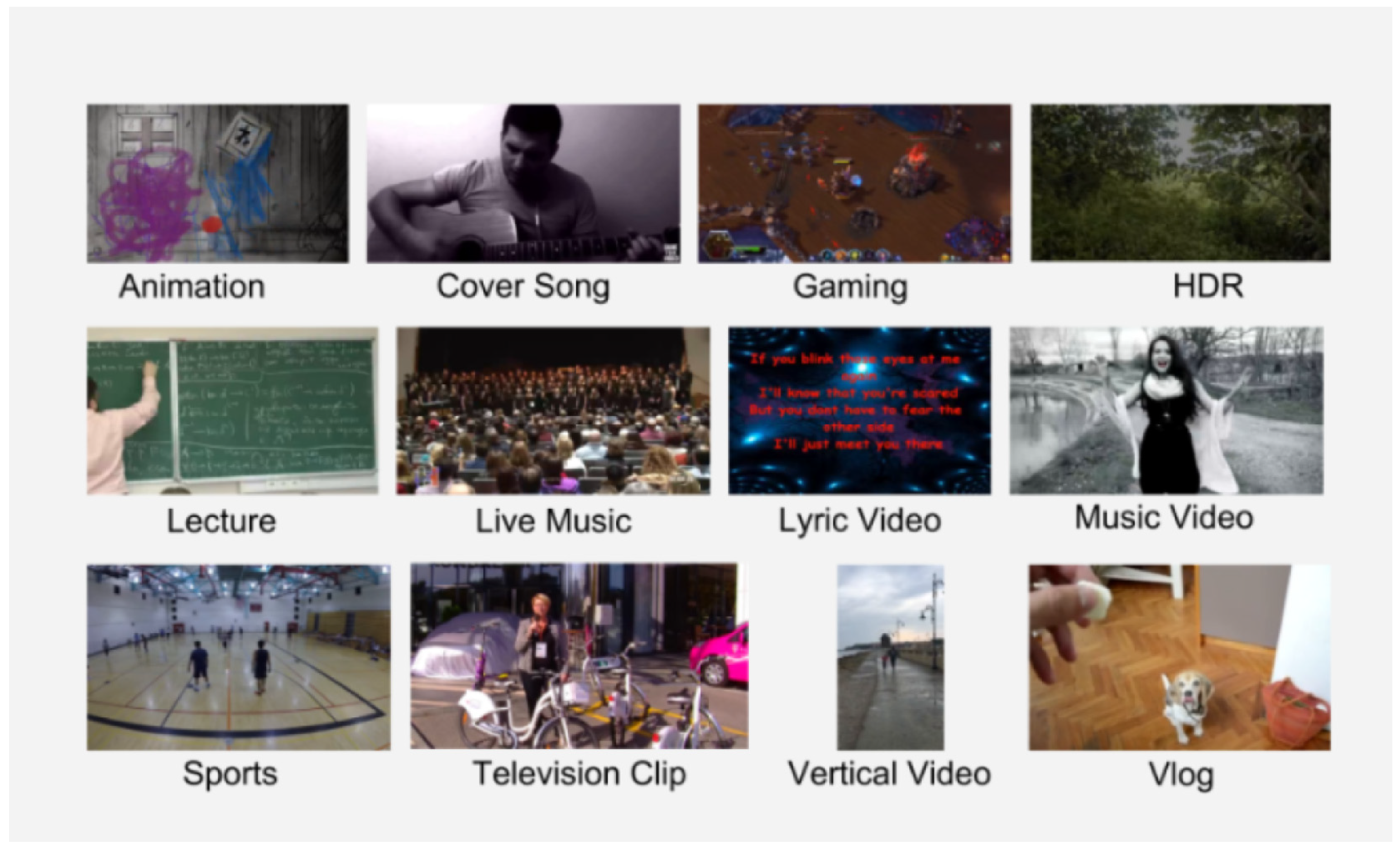
4.1. Search and Description of the Dataset

A large volume of videos to sift through and extract features from is a challenging task, especially given the long duration of some videos, which can last for hours. Our dataset was created by aggregating videos from YouTube, which are licensed under a Creative Commons license [37]. The initial dataset consists of 1.5 million videos divided into 15 categories, each annotated with a knowledge graph [38] (see Figure 1).

The video category is an important attribute in our dataset, making it easier for users to learn the distinctive characteristics of a video. For example, the top ten gaming videos are characterized by fast movement, unlike many lyric videos that show a still background. Using information about this category, compression algorithms can be customized in different ways.

Videos in each category are divided into subgroups based on their resolution. Resolution is an important characteristic that demonstrates different user preferences and differences in the behavior of different devices and platforms. Therefore, it is reasonable to consider resolution as a separate dimension. In our dataset, we used 360P, 480P, 720P, and 1080P resolutions for all categories (except HDR and VR), adding 4K resolution for HDR, gaming, sports, vertical video, vlogs, and VR. The final dataset consists of 1500 video clips, each lasting 20 s. All clips are in Raw YUV 4:2:0 format with a constant frame rate.

4.2. Implementation of Algorithms

In the context of large-scale video compression or transcoding pipelines, lengthy videos are typically divided into segments and encoded concurrently. In practice, preserving quality consistency when transitioning between these segments poses a challenge. Hence, in addition to the three fundamental attributes (spatial, temporal, and color) proposed in [39], we introduce video complexity variation as a fourth attribute, reflecting the intra-segment quality consistency.

We established the duration of video clips in our dataset at 20 s, a length deemed sufficient to encompass various levels of difficulty. These 20 s segments were extracted from random portions of the video. Consequently, out of the 5 million hours of video, there were a staggering 1.8 billion potential 20 s clips. Additionally, we employed Google’s Borg system [40] to encode each video within the initial collection. The encoding was carried out using the FFmpeg H.264 encoder with PSNR enabled. The specific compression settings employed are outlined below:

• constant QP = 20;
• fixed GOP size of 14 frames without B-frames.

The average bitrate in work was determined using the formula:

$$Avarage bitrate=(8\times Initial size)/(Video duration)$$

where $Initial size$—the size of the output file in bytes, 8-bit conversion, $Video duration$—video duration in seconds (in our case, equal to 20 s). After determining the average bitrate, this value was used as the bitrate during encoding. Also, for all Figures 2, 4, 6, 8, and 10, $Initial size$ of video material is equal to 94 Mb. The quality of the obtained videos as a result of applying the appropriate compression methods is shown in Table 2.

To implement the H.265 algorithm, we used the x265 Python library, which is an open-source HEVC encoder that provides a fast and efficient way to encode H.265 video. We used the standard settings of the x265 library to encode our test sequences, which include the standard test sequences from the Joint Collaborative Team on Video Coding (JCT-VC).

In addition to the x265 library, we also used the NumPy library to process and analyze the video data. NumPy is a Python library that provides support for large, multidimensional arrays and matrices commonly used in scientific computing. We used NumPy to load and manipulate video frames, as well as to calculate compression efficiency and visual quality metrics.

Overall, the combination of the x265 and NumPy libraries provided a powerful and flexible platform for implementing and evaluating the H.265 algorithm (see Figure 2).

As you can see from Figure 2, even when using the x265 Python library to implement the H.265 codec and the standard settings of this library, certain details in the image may be lost during video frame compression (look at the upper left corner of both images). First of all, the loss of details can occur due to the characteristics of the compression algorithm itself. Although H.265 is considered to be more efficient than its predecessor, H.264, it is unavoidable that some detail loss will occur during video compression. At high compression ratios, the H.265 algorithm can reduce bitrate and color sampling, which can lead to loss of detail and degradation of image quality. Additionally, if you do not take into account the x265 library settings that can affect compression quality, such as compression level and filtering options, you may risk losing detail in the image. Thus, even with the powerful combination of the x265 and NumPy libraries to implement and analyze the H.265 algorithm, there is a possibility that some image detail may be lost during video frame compression.

Nevertheless, the obtained PSNR (39.17 dB) and SSIM (0.78) values indicate that the H.265 method provides a high-quality compressed video signal, where PSNR indicates a low level of signal loss and SSIM confirms the structural similarity between the original and compressed video.

VP9 is an open-source video compression algorithm developed by Google. It uses various methods to compress video data, including internal prediction, interpretation, transform coding, and entropy coding. The algorithm is designed to provide high compression efficiency while maintaining good video quality.

In our experiment, we implemented the VP9 algorithm using the following Python libraries:

• FFmpeg: A multimedia framework that allowed us to decode and encode video files using the VP9 codec.
• PyAV: A Python wrapper for Ffmpeg that provides a user-friendly interface for manipulating video streams.

To encode video using VP9, we first divided the video into smaller blocks called macroblocks. For each macroblock, we predicted its contents using surrounding blocks and then encoded the difference between the prediction and the original content using transformation. Finally, we encoded the transformed data using entropy coding methods.

To decode video encoded with VP9, we changed the order of operations in reverse order. First, we decoded the entropy-encoded data, applied the inverse transform to recover the transformed data, and then added the estimated content to produce the final reconstructed video.

Overall, our implementation of the VP9 codec using the libvpx library provided efficient video compression with good visual quality (see Figure 3).

For Figure 3, the performance indicators are as follows: PSNR = 38.19 dB, SSIM = 0.79, and the video file size after compression is 22.62 MB. The obtained results demonstrate that both VP9 and H.265 codecs are contemporary and efficient for video compression. The data reveal that H.265 has a slightly higher PSNR but a lower SSIM compared to VP9. Nevertheless, both codecs exhibit significant video compression capabilities, leading to a reduction in file size by more than 70%. When deciding between VP9 and H.265, it is crucial to consider the specific requirements and constraints of your application, including hardware support, quality criteria, network bandwidth, etc. Both codecs present viable options, and the choice may be contingent on the particular conditions and demands of the task.

AV1 is a next-generation video codec that uses advanced technologies such as block splitting and internal and external prediction to achieve high compression efficiency while maintaining high visual quality.

To implement the AV1 codec, we used the following Python libraries:

• NumPy: for efficient array operations and calculations.
• OpenCV: for reading and writing video files, as well as some image processing tasks.

Initially, we generated a compressed bitstream using the AV1 encoder, which takes unedited video as input and outputs the compressed video stream. Then, the AV1 decoder was used to recover the compressed video from the bitstream (see Figure 4).

To evaluate codec performance, we conducted several experiments to measure their compression efficiency and visual quality. We changed coding parameters such as block size, prediction mode, and range of motion vector search.

To compare the performance of VP9 with H.265 and with AV1, we conducted experiments using a dataset of video clips with different resolutions and bitrates. For each clip, the following metrics were measured:

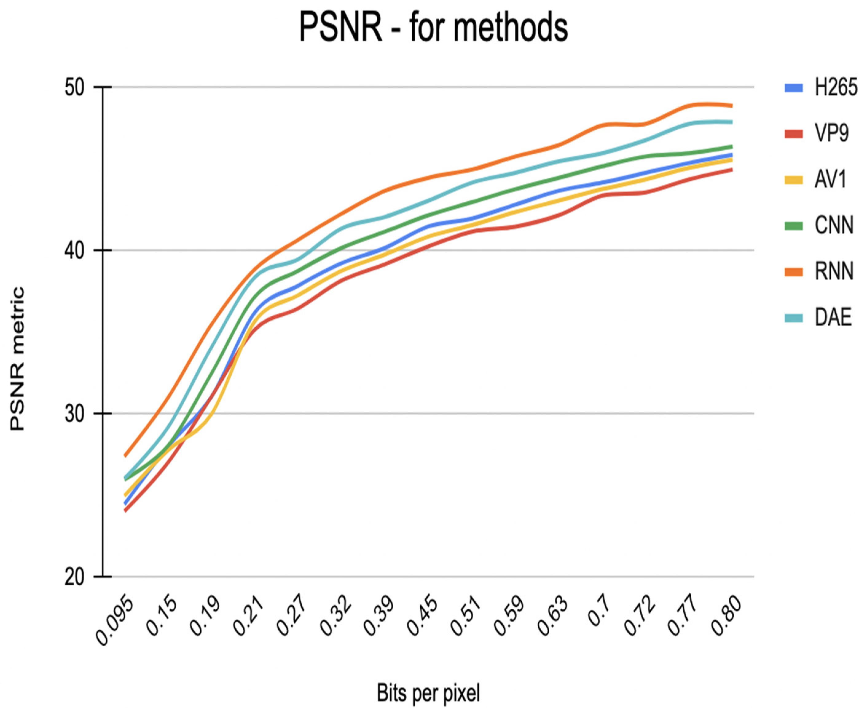
• PSNR: Peak signal-to-noise ratio, which measures the quality of compressed video compared to the original.
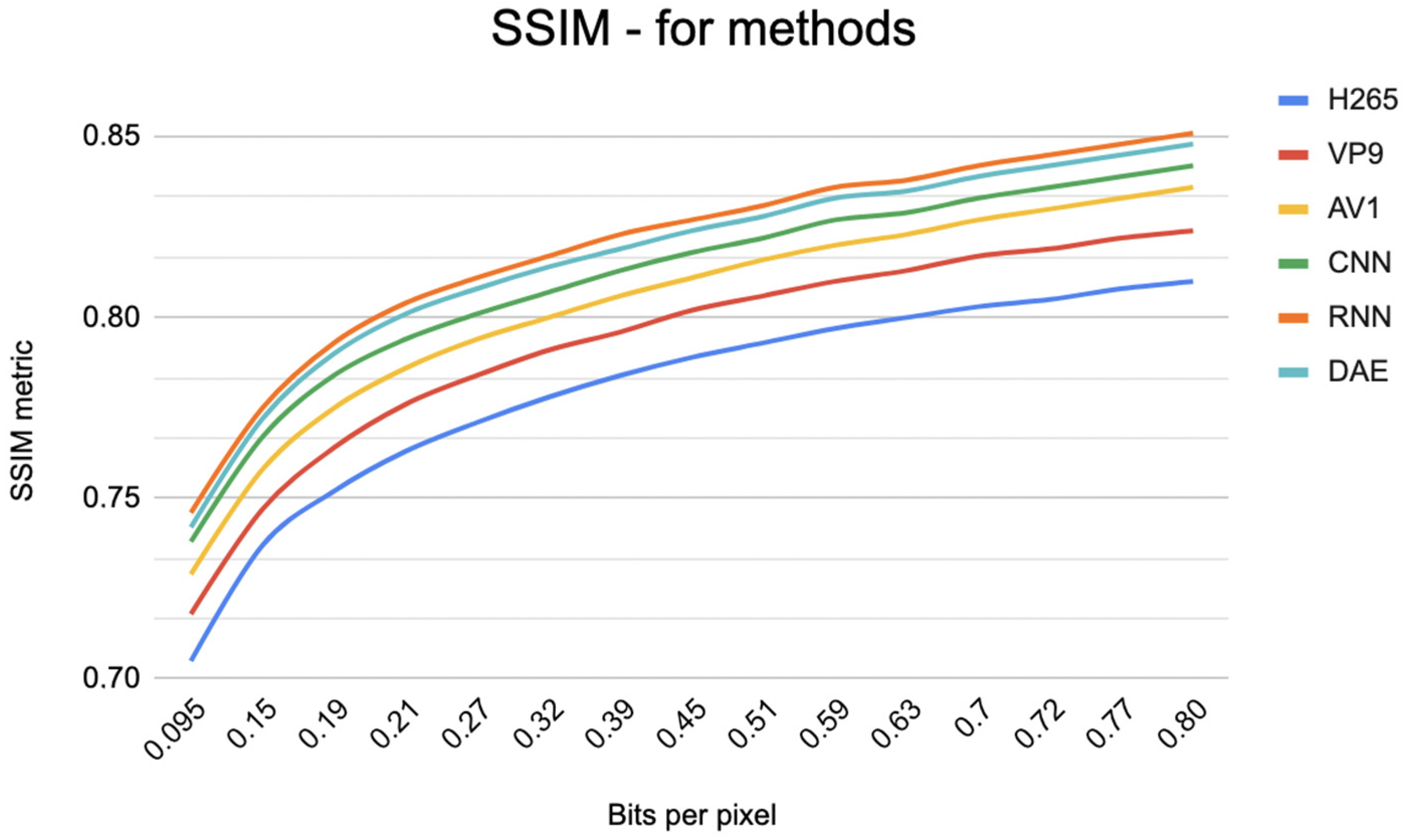
• SSIM: Structural similarity index, which measures the similarity between the compressed video and the original.
• Bitrate: The average number of bits used to represent each frame in a compressed video.

Each clip was encoded using codecs with default settings and recorded PSNR, SSIM, and bitrate for each clip.

To present our results, we created tables and graphs to compare VP9’s performance with H.265 and with AV1. The tables show the average PSNR, SSIM, and bitrate values for each codec in all clips. More details on the results of the experiment can be found in the next section.

Our results showed that all codecs are quite similar in terms of PSNR and SSIM, but VP9 has a slightly lower bit rate for the same video quality.

To build a CNN, we prepared a dataset with a video of the same duration and different resolutions and divided it into training, validation, and test sets. After pre-processing the video by resizing, cropping, and normalizing, we used a CNN architecture with an encoder–decoder structure to compress the incoming video to a smaller-dimensional representation and then reconstruct it with a decoder. We used standard loss functions such as mean square error (MSE) or binary cross entropy (BCE) to measure the difference between compressed and original video.

For model training, we used reverse propagation to update the model weights and optimization algorithms such as stochastic gradient descent (SGD) and Adam. Furthermore, regularization techniques were used, such as dropout and weight reduction, to prevent overfitting. After training, we evaluated the performance of the model on the test set using metrics such as PSNR and SSIM to estimate the visual quality of the compressed video and measure the compression ratio.

The tools we used to implement CNN are Python libraries such as NumPy for efficient array operations and calculations and OpenCV for video processing tasks such as reading and writing video files. In general, our approach was similar to the methodology for implementing video codecs like AV1.

Figure 5 below shows a schematic representation of the architecture used for encoding and decoding.

The architecture presented above (see Figure 5) includes convolutional layers with 3 × 3 filters to extract features from the video, as well as max-pooling layers to reduce dimensionality. Fully connected layers with 1024 neurons are used to further process the features and compress the input data to a lower dimensionality. After encoding, the resulting representation is passed through a decoder to restore the original video. Based on Figure 5, here is the breakdown of processes performed by the encoder and decoder blocks in the given architecture:

Encoder:

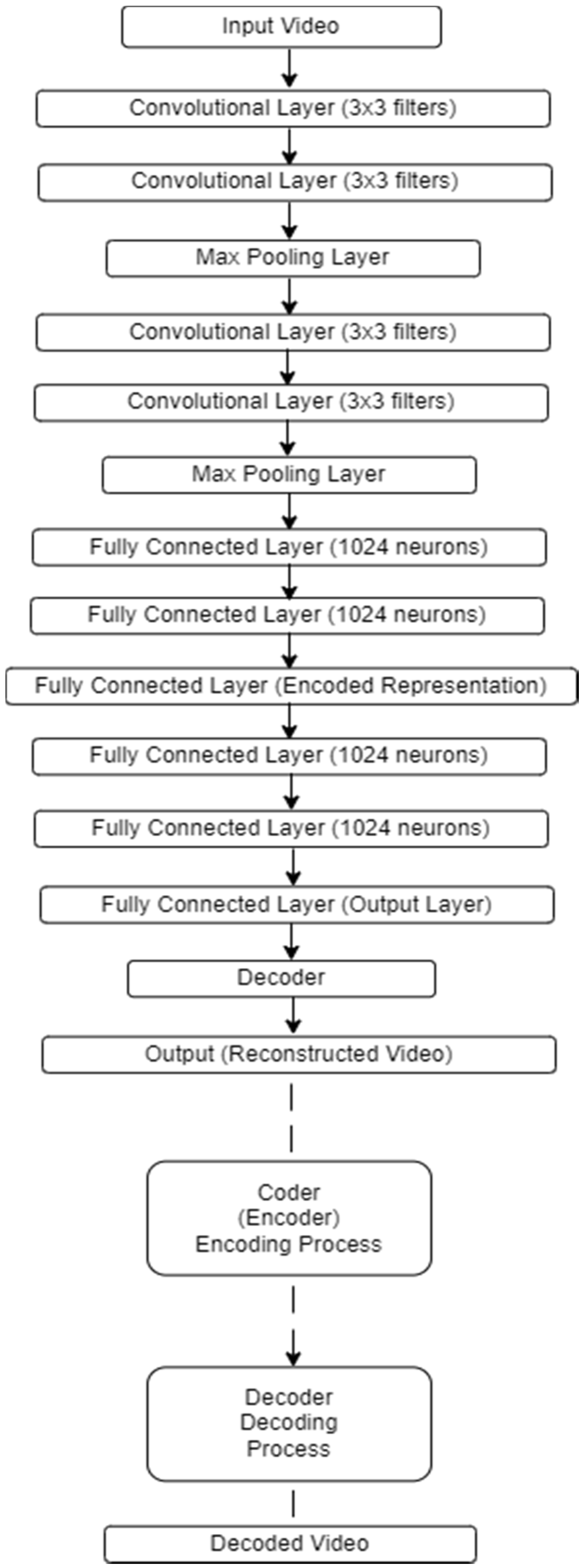
• Convolutional Layers (extract features from the input video clip using 3 × 3 filters).
• Max Pooling Layers (reduce the dimensionality of the extracted features).
• Fully Connected Layers (1024 neurons) (further process the features and compress the input data to a lower dimensionality).
• Fully Connected Layer (encoded representation) (represents the compressed form of the input video clip.

Decoder:

• Fully Connected Layers (1024 neurons) (process the encoded representation.
• Fully Connected Layer (1024 neurons) (further process the features).
• Fully Connected Layer (output layer) (reconstruct the original video clip).
• Mirrors encoder architecture (this implies that the decoder essentially reverses the operations performed by the encoder to reconstruct the original video clip).

To measure the compression efficiency and visual quality of our CNN, we conducted several experiments, as we did when evaluating codecs (see Figure 6). We varied coding parameters such as block size, prediction mode, and motion vector search range to identify areas for improvement and compare our model with other modern methods. As a result, the following optimal options for coding parameters were chosen: Block size 8x8 to ensure finer crushing and more accurate reproduction of features; interframe prediction mode, as it allowed using information from previous frames for prediction and subsequent compression; for optimal use of the motion vector, values ranging from -16 to 16 pixels in the horizontal and vertical directions were used.

To implement an RNN, each video was divided into fixed-length segments and then fed to each segment as a sequence of frames. The RNN encoded the frame sequence into a fixed-length vector representation, which was then used by the RNN decoder to reconstruct the compressed video sequence. We used standard loss functions, such as those of CNN, to measure the difference between the compressed and original video sequences.

For model training, we used backpropagation through time (BPTT) to update the model weights and optimization algorithms such as stochastic gradient descent (SGD) and Adam’s method. Afterward, the training was evaluated on a test set using PSNR and SSIM metrics. To build the RNN, we had to use additional TensorFlow and PyTorch frameworks, unlike CNN.

A general representation of the architecture of the RNN network used for video encoding and decoding with the above parameters is shown in Figure 7.

The effective quantitative values of the coding parameters for the RNN model were as follows:

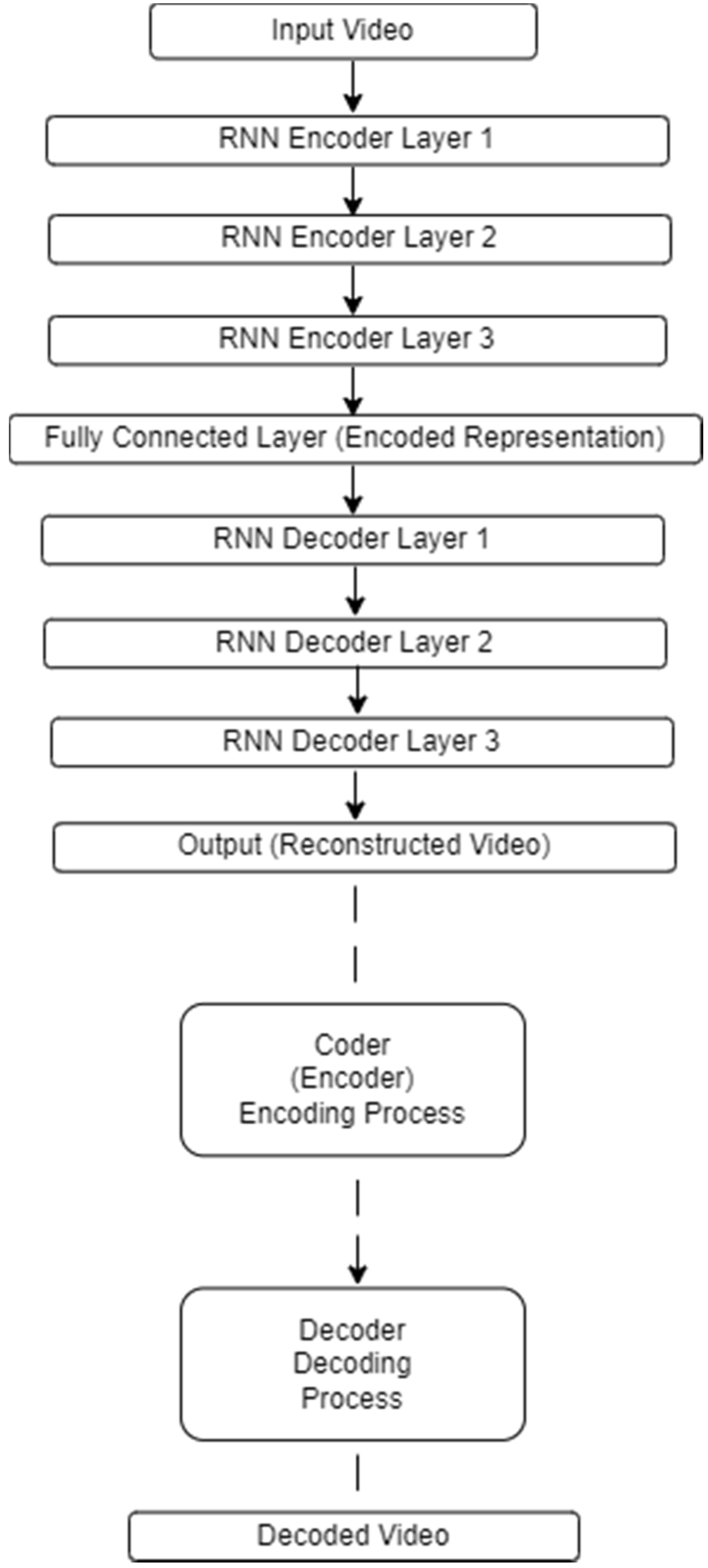
• The sequence length is 20 frames for each fixed video segment.
• The number of layers is equal to 3 layers of RNN coding.
• Each layer has 100 hidden blocks.

In the architecture shown in Figure 7, the processes performed by the encoder blocks:

• Segmentation of the input signal (each video is divided into segments of fixed length).
• Frame sequence encoding (the RNN encoder processes each segment as a frame sequence).
• Feature extraction (layers of the RNN encoder encode the frame sequences into a fixed-length vector representation).
• Compression (a fully connected layer compresses the encoded representations to a smaller size).

And decoder processes:

• Decoding (RNN decoder layers receive the encoded images).
• Sequence recovery (RNN decoder layers recover the compressed video sequence).
• Output generation (the output layer generates the reconstructed video).

In the presented architecture, the RNN encoder encodes sequences of frames into fixed-length vector images, which are then used by the RNN decoder to recover the compressed video sequence.

As with codec estimation and CNN, we conducted several experiments to measure the compression efficiency and visual quality of our RNN (see Figure 8). We varied coding parameters such as sequence length, number of layers, and hidden blocks to identify areas for improvement and compare our model with other modern methods.

The DAE architecture with the encoder–decoder structure is schematically shown in Figure 9. In the given DAE architecture:

Encoder processes:

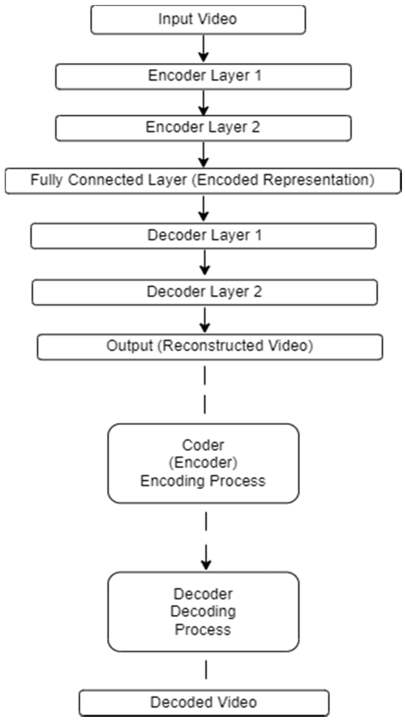
• Input Processing (the input video undergoes pre-processing steps such as resizing, cropping, and normalization).
• Feature Extraction (encoder layers extract features from the pre-processed input video).
• Dimension Reduction (encoder layers progressively reduce the dimensionality of the extracted features).
• Compression (the fully connected layer compresses the encoded representations into a low-dimensional representation).

Decoder processes:

• Decoding (decoder layers receive the low-dimensional representations).
• Feature Expansion (decoder layers expand the low-dimensional representations back to higher dimensions).
• Reconstruction (decoder layers reconstruct the original input video).
• Output Generation (the output layer generates the reconstructed video).

Moreover, to compress the input video to a low-dimensional representation, the DAE architecture with an encoder–decoder structure was used (see Figure 10). The coder part consisted of several convolution and union layers, followed by fully connected layers, while the decoder portion was a mirror reflection of the encoder layers. The input video was pre-processed by resizing, cropping, and normalizing and then divided into training, validation, and test sets. The following effective quantitative parameter values were chosen for the DAE model:

• The number of encoder layers is two.
• The number of decoder layers is also equal to two.

And the size of the fully connected layer (encoded representation) is 256 neurons.

After training, model performance was evaluated on a test set by measuring the compression ratio and using metrics such as PSNR and SSIM to estimate the visual quality of the compressed video.

In general, the DAE method allows you to achieve high compression efficiency with good visual quality and can process videos of different durations. However, it may require more training data and computing resources compared to other methods and may also not be as effective in identifying temporal dependencies in video compared to RNN.

5. Discussion of Results

In this paper, we compare different video compression methods, including codecs, CNNs, RNNs, and deep autoencoders (DAEs), in terms of compression efficiency and visual quality. Several experiments were conducted to evaluate the performance of each method using different video datasets and coding parameters.

To evaluate the methods under consideration, we measured compression efficiency and image quality using metrics such as PSNR and SSIM (see Figure 11 and Figure 12). The results for the codecs showed that all codecs have almost the same PSNR and SSIM, but VP9 has a slightly lower score for the same video quality. Our results also show that the CNN and RNN models performed better than the classical codecs and achieved high compression efficiency and visual quality. However, it should be noted that the RNN model outperformed the CNN model in terms of compression ratio and visual quality. The DAE method also demonstrated high compression efficiency and great visual quality but may require more training data and computing resources compared to other methods.

As a result, all methods showed prospective results in terms of compression efficiency and visual quality. However, the RNN method outperformed the CNN and DAE methods and the classical compression methods.

Based on the research, a comparative table of metrics was formed (see

Table 1. Comparative table of metrics for video compression methods.

Method Name	Average Value PSNR (dB)	Average Value SSIM
H.265	39.17	0.78
VP9	38.19	0.79
AV1	38.72	0.80
CNN	40.00	0.81
RNN	42.05	0.82
DAE	41.15	0.82

) and a quality table (see

Table 2. Comparative table of quality for video compression methods.

Video Material		H.265	VP9	AV1	CNN	RNN	DAE
Number	Initial Size (Mb)	Video File Size after Compression (Mb)
1	50	13.64	13.32	13.34	12.31	9.80	10.71
2	87	21.44	21.12	21.14	20.11	15.91	18.42
3	120	27.84	27.52	26.54	26.51	20.91	24.32
4	75	18.14	17.82	17.10	16.92	13.82	15.51
5	56	14.04	13.72	13.04	12.71	10.13	11.61
6	94	22.94	22.62	21.64	21.62	17.12	19.70

) of different approaches to compressing video materials, as well as describing the positive and negative aspects of each of the proposed methods.

To efficiently compress video using CNN, RNN, and DAE architectures, a video encoder needs trained models. These models are crucial, as they enable the video encoder to perform compression and reconstruction tasks efficiently. Therefore, the size of each model becomes a critical parameter for evaluating the performance and practical implementation of a video compression system. With this in mind,

Table 3. The sizes of the three generated models are in GB.

Initial Size (Mb)	CNN	RNN	DAE
50	1.611	0.928	0.074
87	2.812	1.632	0.129
120	3.841	2.243	0.176
75	2.410	1.408	0.109
56	1.792	1.056	0.082
94	3.008	1.762	0.141

provides an overview of the model sizes corresponding to the initial size of the video material expressed in terms of the amount of memory used. Next, we will consider the advantages and disadvantages of each of the above methods, which will be presented in

Table 4. Comparative table of advantages and disadvantages of video compression methods.

Method Name	Advantages of Using the Method	Disadvantages of Using the Method
H.265	A significant improvement in compression efficiency over its predecessor, H.264. It is supported by many devices and software, making it a widely accepted standard. It supports different video resolutions and frame rates.	In some cases, it may not be as effective as newer codecs such as VP9 and AV1.
VP9	It is open source and does not require royalties, which makes it an attractive option for many companies. Supports high-resolution video and a high frame rate.	It requires more computational resources to encode and decode compared to some other codecs. It is not as widespread as some other codecs, such as H.265.
AV1	It provides significantly better compression efficiency compared to older codecs like H.264 and even newer codecs like H.265 and VP9. It is open source and does not require royalties, which makes it an attractive option for many companies. It supports different video resolutions and frame rates.	It requires more computational resources to encode and decode compared to some other codecs. It is not as common as some other codecs, such as H.265.
CNN	High compression efficiency due to the ability to extract spatial features from video frames. Relatively high coding and decoding speed compared to other deep learning methods. It can work with different resolutions and frame rates.	It may require large computational resources for training and deployment. It is not as effective at detecting temporal dependencies in video as RNN.
RNN	It can effectively capture temporal dependencies in the video, treating each frame as a sequence. It can process video of variable length. It allows you to achieve high compression efficiency with good visual quality.	It may require more time for training and computing resources than CNN. It can be responsive to the length of the input sequence and the choice of hyperparameters.
DAE	It allows you to achieve high compression efficiency with good visual quality. It can process video of variable length. It can be faster and more computationally efficient than other deep learning methods.	It may require more training data and computing resources compared to other methods. It may not be as effective in detecting temporal dependencies in video compared to RNN.

.

In general, each method has its own strengths and weaknesses, and the choice of method depends on the specific requirements and limitations of the video compression task.

The considered methods have several consequences and applications in the field of video compression and storage. One potential application is video streaming, where compressed video can be transmitted over the Internet more efficiently, resulting in faster downloads and less buffering. This could lead to an overall improvement in the user experience for consumers of video streaming services. Furthermore, compressed video can take up less memory space, which can be especially useful for devices with limited memory, such as mobile phones and tablets.

The advantages of the suggested methods are high compression efficiency and good visual quality. The CNN and RNN methods are particularly effective for storing spatial and temporal information, respectively, while the DAE method achieves high compression efficiency with good visual quality and can process videos of different durations. These methods offer a range of video compression options, allowing you to customize them to suit your application’s needs.

Nevertheless, it is important to take into account the limitations. One is that the proposed methods may require more training data and computing resources compared to traditional codecs. Another limitation is that compressed video may not be as compatible as video compressed by traditional codecs, which may limit their practical application in some settings.

Overall, the proposed methods have significant potential to improve the efficiency and quality of video compression and storage, but their practical application will depend on factors such as compatibility and resource requirements.

Despite the results, the proposed method has a number of limitations that should be considered in future research. One major limitation is the size and variety of the dataset used in our experiments. Although we used a variety of publicly available datasets, they may not fully reflect the complexity and diversity of real-world video data. This may have affected the generalizability of our results. Moreover, the computational resources required to train and evaluate models can be quite high, which may limit their practical use in some settings.

Further research should be aimed at eliminating the limitations of the proposed method and improving its performance. One possible direction is to investigate the use of more diverse and realistic datasets to better assess the performance of models. Another focus is to investigate the use of more complex architectures and learning methods to improve the compression efficiency and visual quality of compressed videos. For instance, using attention mechanisms to selectively focus on important video frames and regions can help improve model performance. Eventually, the integration of the proposed method into existing video streaming and storage systems should be explored to determine its practical feasibility.

6. Conclusions

In this paper, several video compression methods have been implemented and evaluated using deep learning techniques. Our results show that these methods can achieve great compression efficiency and high visual quality, making them promising for improving video streaming and storage.

Specifically, we evaluated six methods: H.265, VP9, AV1, CNN, RNN, and DAE. Among them, the CNN and RNN methods proved to be particularly effective in preserving spatial and temporal information, respectively, while the DAE method achieved great compression efficiency with high visual quality and was able to handle videos of different lengths.

Our results showed that deep learning-based methods such as CNN, RNN, and DAE achieved higher compression efficiency and better visual quality compared to traditional codecs such as H.265, VP9, and AV1. The metrics comparison table (Table 1) and quality table (Table 2) provide a comprehensive overview of the performance of each method based on the PSNR and SSIM metrics. Although the proposed methods have significant advantages in terms of compression efficiency and visual quality, there are also limitations to consider, such as the need for more training data and computational resources compared to traditional codecs.

Despite the limitations, our study provides some opportunities for future research. One direction for future research is to use more diverse and realistic datasets to improve the performance evaluation of the model. Another direction is to apply more sophisticated learning architectures and techniques, such as attention mechanisms, to further improve model performance. In addition, further research should explore the feasibility of integrating the proposed methods into existing video streaming and storage systems.

Thus, our study provides a comprehensive evaluation of deep learning methods for video compression. The results demonstrate the potential of these methods to improve video streaming and storage. However, further research is needed to address the limitations of these methods and explore their practical applications. We believe that the results of our study can serve as a guide for future research in this rapidly evolving area.

In summary, our study has shown that deep learning-based methods are a promising direction for improving the efficiency and quality of video compression. By addressing the limitations of these methods and continuing to improve their performance, we will be able to unlock the full potential of video streaming and storage, resulting in more efficient use of storage resources and an improved user experience.

References

1. Chen, W.G.; Yu, R.; Wang, X. Neural Network-Based Video Compression Artifact Reduction Using Temporal Correlation and Sparsity Prior Predictions. IEEE Access 2020, 8, 162479–162490. [Google Scholar] [CrossRef]
2. Havrysh, B.; Tymchenko, O.; Izonin, I. Modification of the LSB Implementation Method of Digital Watermarks. In Advances in Artificial Systems for Logistics Engineering. ICAILE 2022; Lecture Notes on Data Engineering and Communications Technologies; Hu, Z., Zhang, Q., Petoukhov, S., He, M., Eds.; Springer: Cham, Switzerland, 2022; Volume 135, pp. 101–111. [Google Scholar] [CrossRef]
3. Kovtun, V.; Izonin, I.; Gregus, M. Model of functioning of the centralized wireless information ecosystem focused on multimedia streaming. Egypt. Inform. J. 2022, 23, 89–96. [Google Scholar] [CrossRef]
4. Coding of Moving Video: High Efficiency Video Coding (HEVC) ITU-T Recommendation H.265. Available online: https://handle.itu.int/11.1002/1000/14107 (accessed on 1 May 2023).
5. Shilpa, B.; Budati, A.K.; Rao, L.K.; Goyal, S.B. Deep learning based optimised data transmission over 5G networks with Lagrangian encoder. Comput. Electr. Eng. 2022, 102, 108164. [Google Scholar] [CrossRef]
6. Said, A. Machine learning for media compression: Challenges and opportunities. APSIPA Trans. Signal Inf. Process. 2018, 7, e8. [Google Scholar] [CrossRef]
7. Bidwe, R.V.; Mishra, S.; Patil, S.; Shaw, K.; Vora, D.R.; Kotecha, K.; Zope, B. Deep Learning Approaches for Video Compression: A Bibliometric Analysis. Big Data Cogn. Comput. 2022, 6, 44. [Google Scholar] [CrossRef]
8. Zhang, Y.; Kwong, S.; Wang, S. Machine learning based video coding optimizations: A survey. Inf. Sci. 2020, 506, 395–423. [Google Scholar] [CrossRef]
9. Zhou, M.; Wei, X.; Kwong, S.; Jia, W.; Fang, B. Rate Control Method Based on Deep Reinforcement Learning for Dynamic Video Sequences in HEVC. IEEE Trans. Multimed. 2021, 23, 1106–1121. [Google Scholar] [CrossRef]
10. Ji, K.D.; Hlavacs, H. Deep Learning Based Video Compression. In Lecture Notes of the Institute for Computer Sciences, Social Informatics and Telecommunications Engineering; Springer International Publishing: Cham, Switzerland, 2022; pp. 127–141. [Google Scholar]
11. Hoang, T.M.; Zhou, J. Recent trending on learning based video compression: A survey. Cogn. Robot. 2021, 1, 145–158. [Google Scholar] [CrossRef]
12. Dong, C.; Deng, Y.; Loy, C.C.; Tang, X. Compression artifacts reduction by a deep convolutional network. In Proceedings of the IEEE International Conference on Computer Vision, Santiago, Chile, 7–13 December 2015; pp. 576–584. [Google Scholar] [CrossRef]
13. Shao, H.; Liu, B.; Li, Z.; Yan, C.; Sun, Y.; Wang, T. A High-Throughput Processor for GDN-Based Deep Learning Image Compres-sion. Electronics 2023, 12, 2289. [Google Scholar] [CrossRef]
14. Joy, H.K.; Kounte, M.R.; Chandrasekhar, A.; Paul, M. Deep Learning Based Video Compression Techniques with Future Research Issues. Wirel. Pers. Commun. 2023, 131, 2599–2625. [Google Scholar] [CrossRef]
15. Mochurad, L.; Dereviannyi, A.; Antoniv, U. Classification of X-ray Images of the Chest Using Convolutional Neural Networks. IDDM 2021 Informatics & Data-Driven Medicine. In Proceedings of the 4th International Conference on Informatics & Data-Driven Medicine, Valencia, Spain, 19–21 November 2021; pp. 269–282. [Google Scholar]
16. Zhai, D.; Zhang, X.; Li, X.; Xing, X.; Zhou, Y.; Ma, C. Object detection methods on compressed domain videos: An overview, comparative analysis, and new directions. Measurement 2023, 207, 112371. [Google Scholar] [CrossRef]
17. Khuhawar, F.Y.; Bari, I.; Ijaz, A.; Iqbal, A.; Gillani, F.; Hayat, M. Comparative analysis of lossy image compression algorithms. Pak. J. Sci. Res. 2023, 3, 136–147. [Google Scholar]
18. Brown, A.J.; Baburin, A.S. System and Method for Digital Video Management. United. States patent US 7,859,571, 28 December 2010. [Google Scholar]
19. Ameres, E.L.; Bankoski, J.; Grange, A.W.; Murphy, T.; Wilkins, P.G.; Xu, Y. Video Compression and Encoding Method. United. States Patent US 7,499,492, 3 March 2009. [Google Scholar]
20. Wiseman, Y. Video Compression Prototype for Autonomous Vehicles. Smart Cities 2024, 7, 758–771. [Google Scholar] [CrossRef]
21. Klink, J.; Uhl, T. Video Quality Assessment: Some Remarks on Selected Objective Metrics. In Proceedings of the International Conference on Software, Telecommunications and Computer Networks (SoftCOM), Split, Croatia, 17–19 September 2020; pp. 1–6. [Google Scholar]
22. Grois, D.; Nguyen, T.; Marpe, D. Coding efficiency comparison of AV1/VP9, H.265/MPEG-HEVC, and H.264/MPEG-AVC encoders. In Proceedings of the 2016 Picture Coding Symposium (PCS), Nuremberg, Germany, 4–7 December 2016; pp. 1–5. [Google Scholar]
23. Mukherjee, D.; Bankoski, J.; Grange, A.; Han, J.; Koleszar, J.; Wilkins, P.; Xu, Y.; Bultje, R. The latest open-source video codec VP9—An overview and preliminary results. In Proceedings of the 2013 Picture Coding Symposium (PCS), San Jose, CA, USA, 8–11 December 2013; pp. 390–393. [Google Scholar]
24. Yasin, H.M.; Abdulazeez, A.M. Image Compression Based on Deep Learning: A Review. Asian J. Res. Comput. Sci. 2021, 8, 62–76. [Google Scholar] [CrossRef]
25. Nandi, U. Fractal image compression with adaptive quadtree partitioning and non-linear affine map. Multimed. Tools Appl. 2020, 79, 26345–26368. [Google Scholar] [CrossRef]
26. Mochurad, L. Canny Edge Detection Analysis Based on Parallel Algorithm, Constructed Complexity Scale and CUDA. Comput. Inform. 2022, 41, 957–980. [Google Scholar] [CrossRef]
27. Bykov, M.M.; Kovtun, V.V.; Kobylyanska, I.M.; Wójcik, W.; Smailova, S. Improvement of the learning process of the automated speaker recognition system for critical use with HMM-DNN component. In Photonics Applications in Astronomy, Communications, Industry, and High-Energy Physics Experiments; SPIE: Bellingham, WA, USA, 2019. [Google Scholar] [CrossRef]
28. Zhu, S.; Liu, C.; Xu, Z. High-Definition Video Compression System Based on Perception Guidance of Salient Information of a Convolutional Neural Network and HEVC Compression Domain. IEEE Trans. Circuits Syst. Video Technol. 2020, 30, 1946–1959. [Google Scholar] [CrossRef]
29. Kamilaris, A.; Prenafeta-Boldú, F.X. A review of the use of convolutional neural networks in agriculture. J. Agric. Sci. 2018, 156, 312–322. [Google Scholar] [CrossRef]
30. Albahar, M. A Survey on Deep Learning and Its Impact on Agriculture: Challenges and Opportunities. Agriculture 2023, 13, 540. [Google Scholar] [CrossRef]
31. Hu, Y.; Yang, W.; Xia, S.; Cheng, W.H.; Liu, J. Enhanced intra prediction with recurrent neural network in video coding. In Proceedings of the 2018 Data Compression Conference, Snowbird, UT, USA, 27–30 March 2018; p. 413. [Google Scholar]
32. Yu, Y.; Si, X.; Hu, C.; Zhang, J. A Review of Recurrent Neural Networks: LSTM Cells and Network Architectures. Neural Comput. 2019, 31, 1235–1270. [Google Scholar] [CrossRef]
33. Habibian, A.; Rozendaal, T.V.; Tomczak, J.M.; Cohen, T.S. Video Compression with Rate-Distortion Autoencoders. In Proceedings of the IEEE/CVF International Conference on Computer Vision (ICCV), Seoul, Korea, 27 October–2 November 2019; pp. 7032–7041. [Google Scholar] [CrossRef]
34. Toderici, G.; O’Malley, S.M.; Hwang, S.J.; Vincent, D.; Minnen, D.; Baluja, S.; Covell, M.; Sukthankar, R. Variable Rate Image Compression with Recurrent Neural Networks. arXiv 2015, arXiv:1511.06085. [Google Scholar]
35. Horé, A.; Ziou, D. Image Quality Metrics: PSNR vs. SSIM. In Proceedings of the 2010 20th International Conference on Pattern Recognition, Istanbul, Turkey, 23–26 August 2010; pp. 2366–2369. [Google Scholar]
36. Setiadi, D.R.I.M. PSNR vs. SSIM: Imperceptibility quality assessment for image steganography. Multimed. Tools Appl. 2021, 80, 8423–8444. [Google Scholar] [CrossRef]
37. YouTube. YOUTUBE UGC Dataset. 2021. Available online: https://media.withyoutube.com/ (accessed on 13 April 2024).
38. Singhal, A. Introducing the Knowledge Graph: Things, Not Strings. 2012. Available online: https://blog.google/products/search/introducing-knowledge-graph-things-not/ (accessed on 13 April 2024).
39. Winkler, S. Analysis of Public Image and Video Databases for Quality Assessment. IEEE J. Sel. Top. Signal Process. 2012, 6, 616–625. [Google Scholar] [CrossRef]
40. Verma, A.; Pedrosa, L.; Korupolu, M.; Oppenheimer, D.; Tune, E.; Wilkes, J. Large-scale cluster management at Google with Borg. In Proceedings of the Tenth European Conference on Computer Systems (EuroSys 1‘5), Association for Computing Machinery, New York, NY, USA, 21–24 April 2015; Article number 18. pp. 1–17. [Google Scholar] [CrossRef]
Figure 1. Video categories in the YouTube UGC dataset.
Technologies 12 00052 g001
Figure 2. Video frame from the dataset: (a) before and (b) after compression using H.265.
Technologies 12 00052 g002
Figure 3. Video frame from the dataset: (a) before and (b) after compression with VP9.
Technologies 12 00052 g003
Figure 4. Video frame from the dataset: (a) before and (b) after compression with AV1.
Technologies 12 00052 g004
Figure 5. CNN network architecture for video encoding and decoding.
Technologies 12 00052 g005
Figure 6. Video frame from the dataset: (a) before and (b) after compression using a CNN.
Technologies 12 00052 g006
Figure 7. RNN network architecture for video encoding–decoding.
Technologies 12 00052 g007
Figure 8. Video frame from the dataset: (a) before and (b) after compression using an RNN.
Technologies 12 00052 g008
Figure 9. The DAE architecture with the encoder–decoder structure.
Technologies 12 00052 g009
Figure 10. Frame video from the dataset: (a) before and (b) after compression using DAE.
Technologies 12 00052 g010
Figure 11. Graph of estimation of video compression methods based on PSNR metric.
Technologies 12 00052 g011
Figure 12. Graph of evaluation of video compression methods based on SSIM metric.
Technologies 12 00052 g012