Using Principal Component Analysis for Temperature Readings from YF₃:Pr³⁺ Luminescence

Abstract

The method of measuring temperature using luminescence by analyzing the emission spectra of Pr³⁺-doped YF₃ using principal component analysis is presented. The Pr³⁺-doped YF₃ is synthesized using a solid-state technique, and its single-phase orthorhombic crystal structure is confirmed using X-ray diffraction. The emission spectra measured within the 93–473 K temperature range displays characteristic Pr³⁺ f-f electronic transitions. The red emission from the ³P_0,1→³H₆,³F₂ electronic transition mostly dominates the spectra. However, at low temperatures, the intensity of the green emissions from the ³P_0,1→³H₅, deep-red ³P_0,1→³F₄, and the deep-red emissions from the ³P_0,1→³F₄ transitions are considerably lower compared to the intensity of the red emissions. Temperature variations directly impact the photoluminescent spectra, causing a notable increase in the green and deep-red emissions from the ³P₁ excited state. We utilized the entire spectrum as an input for principal component analysis, considering each temperature as an independent group of data. The first principal component explained 99.3% of the variance in emission spectra caused by temperature and we further used it as a reliable temperature indicator for luminescence thermometry. The approach has a maximum absolute sensitivity of around 0.012 K⁻¹. The average accuracy and precision values are 0.7 K and 0.5 K, respectively.

1. Introduction

Temperature is a crucial variable in numerous scientific, industrial, and technological domains, aiding in comprehending physical phenomena and enhancing system effectiveness. Thermometry, the practice of measuring temperature, is presently carried out using several technologies that rely on distinct approaches to measurement. With the increasing demand for precise temperature measurements, there is a pressing requirement to develop novel thermosensitive materials and more accurate temperature read-outs. There is a strong requirement for noncontact thermometry in situations when objects are in motion, sensitive to touch, hard to reach, or located in hazardous places. Temperature measurements that utilize variations in the optical characteristics of materials are regarded as promising for addressing needs. Among these methods, luminescence thermometry, which involves studying the temperature dependencies of the luminescent properties of materials, has garnered the greatest attention [1,2,3,4].

Luminescence thermometry is a remote sensing technique that uses the temperature dependence of a phosphor’s luminescence properties (e.g., band shape, peak energy or intensity, excited state durations, and risetimes) to determine temperature. This technology gives precise thermal readouts with high spatial resolution in a short acquisition time. It has significant potential in various fields, including optoelectronics, photonics, micro- and nanofluidics, and nanomedicine. Luminescent thermometry’s challenges include the ongoing search for and development of novel materials, experimental techniques, and analysis procedures to increase the technology’s competitiveness and accessibility [1,2,3,4]. Researchers reported numerous luminescence temperature probes and read-out methods; however, there is always room for improvement in the performance of thermometry that can be achieved through the following: (i) innovative approaches in temperature read-outs and experimental techniques; (ii) the development of novel luminescent probes; (iii) the extension of theoretical models and a careful re-examination of those currently in use; and (iv) novel analysis procedures [5,6,7,8].

To determine temperature, luminescence thermometry uses the temperature dependence of different phosphors’ luminescence properties. For example, luminescence intensity ratio (LIR) measurements are based on temperature-induced changes in the intensity ratio between two spectral lines. Band shift and bandwidth measurements focus on temperature-induced band shape and position changes. However, all these read-outs utilize only a fraction of the data within the spectral lines, concentrating predominantly on the properties of individual spectral lines. Recently, researchers have attempted to enhance the method by merging multiple thermometric parameters into a single multiparametric temperature readout (MLR). This approach aims to leverage machine learning techniques like neural networks [9,10], dimensionality reduction (DR) methods like principal component analysis (PCA) [11,12], and nonlinear DR methods like t-distributed stochastic neighbor embedding (t-SNE) [11]. All these approaches focus on combining thermometric parameters, but not the complete temperature-induced spectral change, omitting a significant portion of luminescence features from temperature determination.

Machine learning is a branch of artificial intelligence focused on developing algorithms that enable computers to learn from and make data-based decisions. By analyzing patterns and iteratively improving their performance, machine learning models can automate tasks ranging from image recognition and natural language processing to medical diagnosis and agriculture [13,14,15,16]. Techniques such as supervised learning, unsupervised learning, and reinforcement learning drive advancements in robotics, healthcare, and finance. The field’s rapid growth is fueled by increasing data availability and computational power, promising innovations that reshape industries and everyday life through more accurate predictions and autonomous systems.

Here, we aimed to exploit principal component analysis, an unsupervised learning method, for obtaining temperature indicators for luminescent thermometry. We hypothesize that by using the maximum amount of temperature-induced variance in luminescence emission spectra, one can obtain the best possible sensitivity of the method. To achieve this, we suggest using the complete emission spectrum of the luminescence thermometry probe, which is measured multiple times at different temperatures. We then employ the principal component analysis algorithm to transform the data from high-dimension to low-dimension space, while preserving the meaningful properties of the original data. Furthermore, this approach eliminates the need to determine the spectral features and spectral regions suitable for temperature measurements from luminescence, which is a requirement in conventional approaches, as we use the entire spectrum for the measurement. We present here the synthesis, structural, morphological, and photoluminescent properties of the Pr³⁺-doped YF₃ luminescence thermometry probe material and the thermometric performance of the luminescence thermometry method based on the principal component analysis.

2. Materials and Methods

The following chemicals were used to prepare 0.2 mol% Pr³⁺-doped YF₃ (Y_0.998Pr_0.002F₃): yttrium oxide (Y₂O₃, Sigma-Aldrich, St. Louis, MO, USA, 99.99%), praseodymium oxide (Pr₆O₁₁, Sigma-Aldrich, 99.99%), and ammonium hydrogen difluoride (NH₄HF₂, Sigma-Aldrich, 98.5%). To synthesize the Y_0.998Pr_0.002F₃ sample, the stoichiometric amounts of Y₂O₃ and Pr₆O₁₁ were mixed with NH₄HF₂. The obtained mixture was thoroughly ground in an agate mortar to ensure the best homogeneity and then heated, first in the air at 170 °C for 20 h and then at 500 °C for 3 h in a slightly reducing atmosphere (Ar-10% H₂).

An X-ray diffractometer (XRD) from Rigaku SmartLab was used to investigate the crystal structures of the powders. The diffractometer operated with Cu-Kα_1,2 radiation at a wavelength of λ = 0.1540 nm under room temperature settings. The measurements were conducted within the 2θ range of 10° to 90°, with a step size of 0.02°, and a counting rate of 10° per minute. The morphology of the material was analyzed using a TESCAN MIRA3 field emission gun scanning electron microscope (SEM). The samples were coated with a thin layer of gold using a conventional sputtering technique (Polaron SC502; Fison Instruments, Glasgow, UK). The determination of particle size distribution was conducted using the IMAGEJ program. The Fluorolog-3 Model FL3-221 spectrofluorometer equipment (Horiba Jobin-Yvon, Palaiseau, France) was used to measure the excitation spectra. Temperature-dependent emission spectra were measured using the Ocean FX UV-VIS Spectrometer with the excitation light source (450 nm Ocean Insight LED module) working continuously and controlled using LDC-1. The temperature of the samples was controlled by using a MicroOptik liquid nitrogen-cooled heating–cooling stage. Once the temperature was stabilized, a series of 100 spectra was measured for each temperature.

In this approach, spectroscopic data are utilized by treating the intensity at specific wavelengths as variables, so the number of variables equals the number of spectral points (N_SP = 598). As a result, each spectrum can be assigned to a single point within a hyperspace of dimensionality N_SP. Then, principal component analysis (PCA) is used to identify N_SP principal components (PCs), with only the first few providing significant information. The principal components (PCs) are linear combinations of the original variables, designed to be orthogonal and have decreasing variance. The first principal component has the highest variance, while the subsequent ones have progressively lower variance across their axes (s_PC1 > s_PC2> … >s_PCi > s_PCi+1…). Each spectrum (Sj) is associated with its corresponding temperature (Tj), yielding a [Sj, Tj] pair that can be seen as a hypercloud of Sj spectra/dots.

3. Results and Discussion

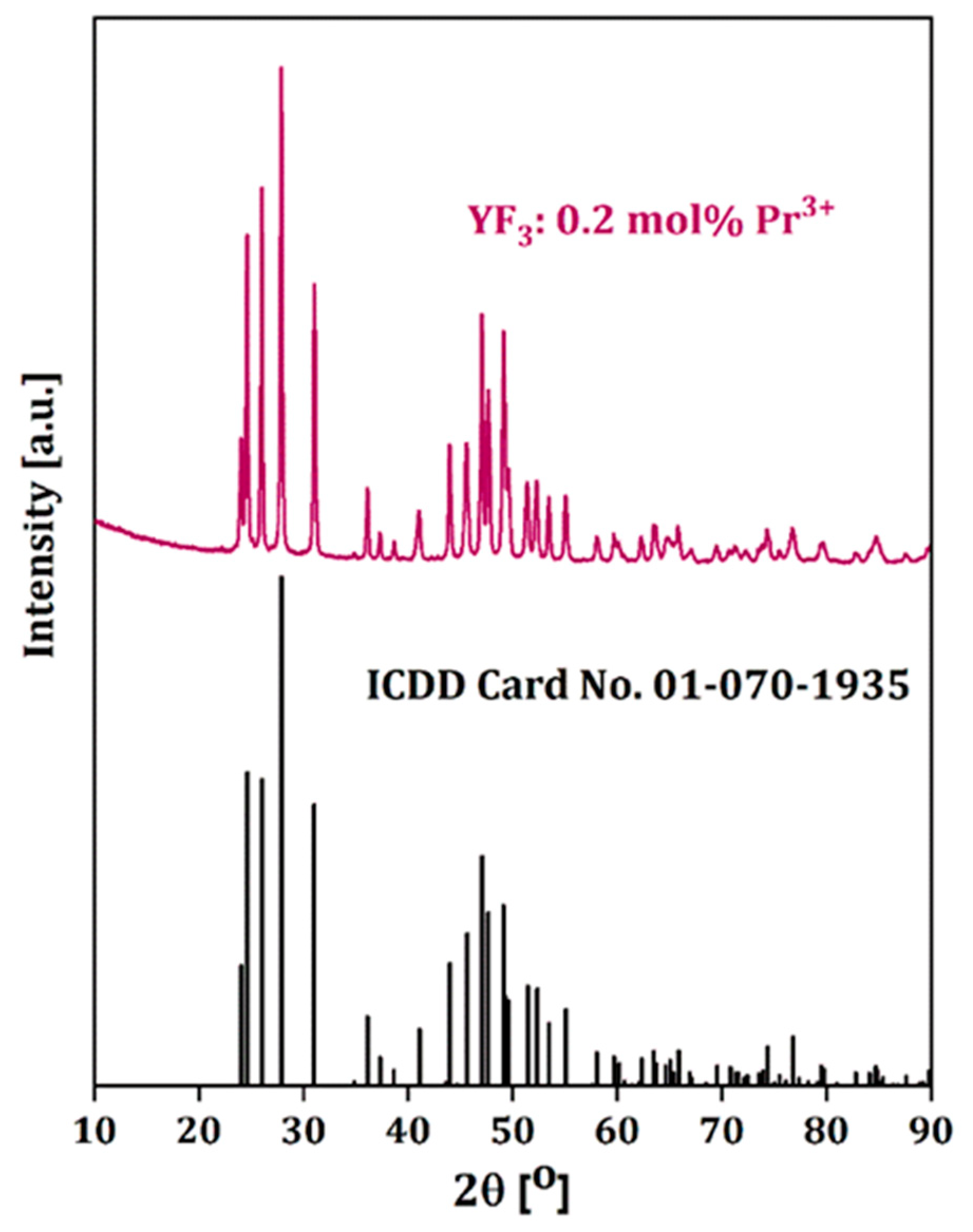
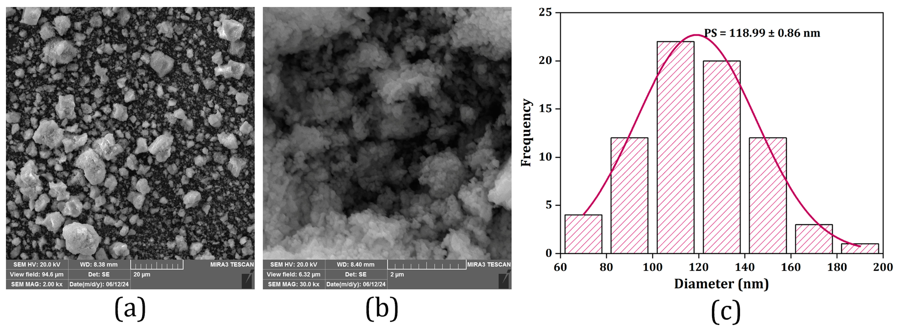
3.1. Structural and Morphological Analysis

Figure 1 shows the X-ray diffraction pattern of synthesized Pr³⁺-doped YF₃ with the plotted data of corresponding ICDD Card No. 01-070-1935. The diffractogram shows a single-phase orthorhombic crystal structure having a Pnma space group. In this space group, Y³⁺ is nine-coordinated with fluoride ions, having an ionic radius of ${\mathrm{Y}}_{IX}^{3+}$ = 1.075 Å [17]. No additional reflections in the X-ray diffraction pattern confirm the successful incorporation of similar-size Pr³⁺ (${\mathrm{P}\mathrm{r}}_{IX}^{3+}$ = 1.179 Å, [17]). According to the structural parameters analysis obtained from XRD measurements using build-it software, the mean crystallite size and microstrain of the Y_0.998Pr_0.002F₃ sample are ~29 nm and 0.05%, respectively. Also, the calculated cell parameters are a = 6.3532(2) Å, b = 6.8566(2) Å, and c = 4.40470(17) Å, and these values are in good agreement with the values of cell parameters for YF₃ from the literature [18].

Scanning electron microscopy was performed to investigate the morphology and particle size distribution of the obtained Pr³⁺-doped YF₃ powder. The representative images with low and high magnifications are given in Figure 2. The low-magnification image in Figure 2a shows that the powder is composed of different micron-sized chunks, which, under higher magnification (Figure 2b), show nanosized particles with similar quasi-spherical shapes. Figure 2c presents the calculated average particle size of approximately 120 nm based on 75 particles.

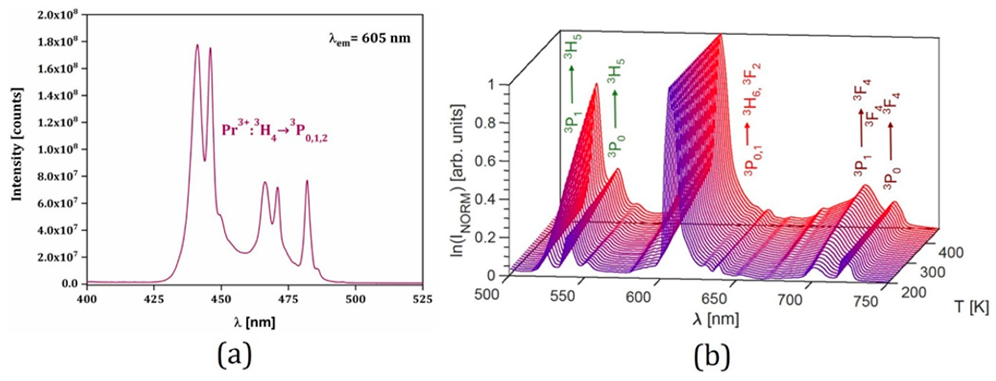
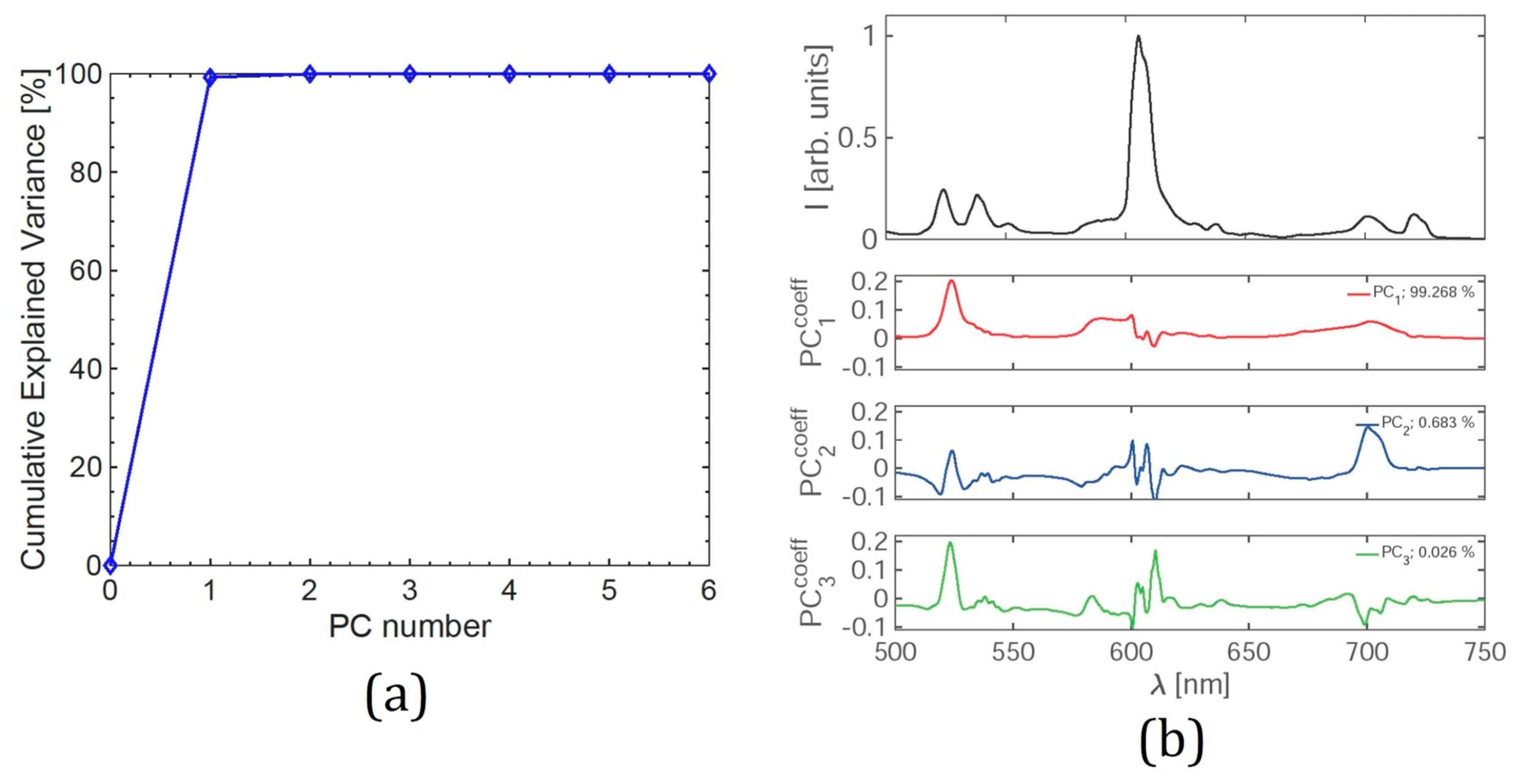
3.2. Temperature-Dependent Photoluminescent Properties

Pr³⁺ exhibits resourceful luminescence in a spectral range from ultraviolet, visible to infrared, due to its 4f5d→4f² inter-configurational and 4f²→4f² intra-configurational emission transitions that are significantly influenced by host materials [19]. Figure 3a presents the excitation spectrum of the Pr³⁺-doped YF₃ (λ_em = 605 nm) sample showing Pr³⁺ absorptions from ³H₄$\to$³P_0,1,2 transitions in the blue spectral range. Figure 3b shows temperature-dependent photoluminescent emission spectra recorded from 200 K to 473 K. They reveal typical emissions corresponding to 4f²→4f² transitions within Pr³⁺ [20]. After excitation with 450 nm radiation, emissions from the first six excited levels are present in the spectral range from 450 nm to 750 nm [21,22,23]. The spectra are dominated by red emission from ³P_0,1→³H₆,³F₂ transitions around 610 nm. The green ³P_0,1$\to$³H₅, and deep-red ³P_0,1$\to$³F₄ emissions are of much smaller intensity than the red emissions at low temperatures. No transition originating from the ¹D₂ state can be observed under regular excitation in the ³P_J multiplets. As anticipated, the width of emission lines increases with increasing temperatures, and the relative strength varies due to the differing occupation of the various sublevels and absorption efficiency [21]. Hot bands start to appear, but their intensity is too weak to be easily observed. As a result, the sample’s photoluminescent spectra show multiple temperature-induced changes. Some of them are strongly pronounced, and some of them are less so. When such a variety of temperature-caused changes in the emission spectrum exist, one can assume that not all of them can be captured for thermometry with standard luminescence temperature indicators such as the luminescence intensity ratio, bandwidth, and band shift, and the use of the entirety of the spectrum becomes justified. One method that can achieve this is PCA.

We preprocessed all emission spectra, which involved background removal and normalization, setting the maximum intensity value for each spectrum to 1, in order to determine the thermographic potential of the Pr³⁺-doped YF₃ sample and to test the performance of the PCA method. For the PCA, the spectra measured at each temperature were treated as a part of the same group.

We applied PCA using a randomly selected half of the spectra at each temperature from the entire dataset. We acquired 3900 total measured spectra (100 spectra for each of the 39 stabilized temperatures), using half (50 per temperature, a total of 1950) for PCA and the other half for testing and verification. This procedure produced 598 principal components (${PC}_i;1\le i\le 598$); each $({PC}_i$) is accompanied by a coefficient vector ${PC}_i^{coeff}$, which we can calculate as a scalar product between a coefficient vector and a spectrum vector, with N_SP being the number of spectra. Since each spectrum is associated with a temperature, the same holds for each calculated ${PC}_i$, as given by the following equation:

$${PC}_i\left(T_k\right)={PC}_i^{coeff}·I(T_k)={\sum }_{j=1}^{N_{SP}}{PC}_i^{coeff}\left({\lambda }_j\right)I({\lambda }_j,T_k)$$

(1)

Figure 4a displays the percentage of temperature-induced variance in emission spectra that principal components cumulatively explain. In the case under consideration, only one principal component was sufficient enough to capture almost the entire variance. Figure 4b shows a typical emission spectrum (top graph), while values for the ${PC}_1^{coeff}$, ${PC}_2^{coeff},$ and ${PC}_3^{coeff}$ coefficient vectors with their significance are shown on lower graphs. The highest influence weight of ~99.3% is ${PC}_1$, while the next parametric component, ${PC}_2$, has ~0.7% influence. The third principal component has an almost negligible influence. In addition, according to the coefficient values, the whole emission spectrum contributes to ${PC}_1$. However, the largest contribution comes from the spectral regions where emissions from the f-f electronic transitions occur. These are the consequences of temperature quenching the emissions, the thermalization of higher-energy excited states, the appearance of hot bands, etc.

Here, we used PC₁ as a temperature indicator for luminescence thermometry. It can be used in the same way as the luminescence intensity ratio, band shift, bandwidth, or excited state lifetime. Figure 5a plots the average value at each temperature against temperature (diamonds). The red line represents the polynomial fit to the experimental data. The temperature dependence is a monotonic function, which is a prerequisite for temperature determination.

The absolute and relative sensitivities of the PCA-based luminescence thermometry method, S_a and S_r, shown in Figure 5b,c, are determined using the following equation:

$$S_a=\left|{\displaystyle \frac{\mathrm{d}{PC}_1}{\mathrm{d}T}}\right|, S_r={\displaystyle \frac{1}{{PC}_1}}\left|{\displaystyle \frac{\mathrm{d}{PC}_1}{\mathrm{d}T}}\right|\times 100\%.$$

(2)

Based on the mean value of all at the corresponding nominal temperature plots, the maximal absolute sensitivity of the method is ~0.012K⁻¹. The relative sensitivity value decreases with temperature, from 0.84%K⁻¹ at 200 K to 0.25%K⁻¹ at 473 K. Temperature accuracy (ΔT) and precision (δT) are the most important thermometric parameters in luminescence thermometry. To calculate precision and accuracy, the spectra that were not employed in the PCA were considered to produce the distribution of PC₁ on corresponding temperatures and thus experimentally obtain the values for ΔT and δT. At each nominal temperature T, there are N_VAL = 50 spectra measured and utilized for testing and verification. The values for ${PC}_{1,i}(T)$, and then T_i(T) (where I = 1 to N_VAL), were derived using Equation (1). Equation (3) gives us the accuracy degree at that temperature, ΔT(T), which is the mean value of the difference between the measured and nominal temperature values. On the other hand, Equation (4) gives us the precision or temperature resolution value at the same nominal temperature, δT(T), which is the spread (standard deviation) of the T_i(T) distribution. The temperature dependency of both ΔT (circles) and δT (diamonds) is shown in Figure 5d (left y axes).

$$∆T\left(T\right)={\displaystyle \frac{1}{N_{VAL}}}{\sum }_{i=1}^{N_{VAL}}\left|{T-T}_i\left(T\right)\right|=\left|T-{\displaystyle \frac{1}{N_{VAL}}}{\sum }_{i=1}^{N_{VAL}}{T}_i\left(T\right)\right|=\left|T-\overline{T_i\left(T\right)}\right|,$$

(3)

$$\delta T(T)=\sqrt{{\displaystyle \frac{1}{N_{VAL}-1}}{\sum }_{i=1}^{N_{VAL}}{\left|T_i\left(T\right)-\overline{T_i\left(T\right)}\right|}^2}$$

(4)

Based on the mean value of all at the corresponding nominal temperature plots, the average values for accuracy and precision are 0.7 K and 0.5 K, respectively. It should be noted here that the accuracy and precision values are heavily dependent on uncertainty in emission spectra measurements. In this research, we used a low-cost fiber-optic instrument. Higher-quality instruments, which provide lower values of measurement uncertainty, could yield much better accuracy and precision.

4. Conclusions

Machine learning for sensors involves leveraging algorithms and statistical models to interpret sensor data. Principal component analysis is a dimensionality reduction technique that transforms high-dimensional data into a set of linearly uncorrelated variables called principal components. By capturing the variance in the original data in decreasing order, these components preserve the most significant patterns or features while discarding less informative aspects. We employed a principal component analysis machine learning algorithm for luminescence thermometry, utilizing the steady-state visible emission from Pr³⁺. We find that the first principal component carries almost all the influence weight (99.3%), with contributions from all spectral parts. From the mean values of all the corresponding nominal temperature plots, the maximal absolute sensitivity is calculated to be ~0.012K⁻¹, while the values for accuracy and precision are 0.7 K and 0.5 K, respectively.

The approach has the following advantages:

This approach distinguishes itself from other more complex methods, such as artificial neural networks and multiparameter regressions, by using only the basic mathematical operations of addition and multiplication.

Using the PCA method after calibration is much easier than other methods such as multiparametric readout (MLR), which need complicated calculations to process data to find different LIRs, band positions, and especially MLR. This makes the process a lot easier. To apply PCA, we can simply multiply the associated principal component vector by the normalized spectrum intensity vector.

Overall, machine learning enhances the capabilities of sensors by enabling them to learn, adapt, and provide intelligent insights from the data they collect, thereby contributing to smarter and more efficient systems across various domains. The extent to which these findings can be generalized in luminescence thermometry remains a topic for future investigation, particularly in exploring different combinations of temperature readings and luminescent centers.

References

1. Dramićanin, M. Luminescence Thermometry: Methods, Materials, and Applications, 1st ed.; Elsevier: Amsterdam, The Netherlands, 2018. [Google Scholar] [CrossRef]
2. Carvajal Martí, J.J.; Pujol Baiges, M.C. (Eds.) Luminescent Thermometry Applications and Uses; Springer: Cham, Switzerland, 2023. [Google Scholar]
3. Đačanin Far, L.; Dramićanin, M.D. Luminescence thermometry with nanoparticles: A review. Nanomaterials 2023, 13, 2904. [Google Scholar] [CrossRef]
4. Brites, C.D.S.; Balabhadra, S.; Carlos, L.D. Lanthanide-based thermometers: At the cutting-edge of luminescence thermometry. Adv. Opt. Mater. 2018, 7, 1801239. [Google Scholar] [CrossRef]
5. Brites, C.D.S.; Marin, R.; Suta, M.; Carneiro Neto, A.N.; Ximendes, E.; Jaque, D.; Carlos, L.D. Spotlight on luminescence thermometry: Basics, challenges, and cutting-edge applications. Adv. Mater. 2023, 35, 2302749. [Google Scholar] [CrossRef] [PubMed]
6. Zhang, B.; Guo, X.; Zhang, Z.; Fu, Z.; Zheng, H. Luminescence thermometry with rare earth doped nanoparticles: Status and challenges. J. Lumin. 2022, 250, 119110. [Google Scholar] [CrossRef]
7. Bednarkiewicz, A.; Drabik, J.; Trejgis, K.; Jaque, D.; Ximendes, E.; Marciniak, L. Luminescence based temperature bio-imaging: Status, challenges, and perspectives. Appl. Phys. Rev. 2021, 8, 011317. [Google Scholar] [CrossRef]
8. Dramićanin, M.D. Trends in luminescence thermometry. J. Appl. Phys. 2020, 128, 040902. [Google Scholar] [CrossRef]
9. Lewis, C.; Erikson, J.W.; Sanchez, D.A.; McClure, C.E.; Nordin, G.P.; Munro, T.R.; Colton, J.S. Use of machine learning with temporal photoluminescence signals from CdTe quantum dots for temperature measurement in microfluidic devices. ACS Appl. Nano Mater. 2020, 3, 4045–4053. [Google Scholar] [CrossRef] [PubMed]
10. Cai, T.; Deng, Z.; Park, Y.; Mohammadshahi, S.; Liu, Y.; Kim, K.C. Acquisition of kHz-frequency two-dimensional surface temperature field using phosphor thermometry and proper orthogonal decomposition assisted long short-term memory neural networks. Int. J. Heat Mass Transf. 2021, 165, 120662. [Google Scholar] [CrossRef]
11. Ximendes, E.; Marin, R.; Carlos, L.D.; Jaque, D. Less is more: Dimensionality reduction as a general strategy for more precise luminescence thermometry. Light Sci. Appl. 2022, 11, 237. [Google Scholar] [CrossRef]
12. Šević, D.; Vlašić, A.; Rabasović, M.S.; Savić-Sević, S.; Rabasović, M.; Nikolić, M.G.; Murić, B.; Marinković, B.; Križan, J. Temperature effects on luminescent properties of Sr2CeO4:Eu3+ nanophosphor: A machine learning approach. Tehnika 2020, 75, 279–283. [Google Scholar] [CrossRef]
13. Aoun, N.B. A Review of automatic pain assessment from facial information using machine learning. Technologies 2024, 12, 92. [Google Scholar] [CrossRef]
14. Manakitsa, N.; Maraslidis, G.S.; Moysis, L.; Fragulis, G.F. A Review of machine learning and deep learning for object detection, semantic segmentation, and human action recognition in machine and robotic vision. Technologies 2024, 12, 15. [Google Scholar] [CrossRef]
15. González-Rodríguez, J.-R.; Córdova-Esparza, D.-M.; Terven, J.; Romero-González, J.-A. Towards a bidirectional Mexican sign language–Spanish translation system: A deep learning approach. Technologies 2024, 12, 7. [Google Scholar] [CrossRef]
16. Bakthavatchalam, K.; Karthik, B.; Thiruvengadam, V.; Muthal, S.; Deepa, J.; Kotecha, K.; Varadarajan, V. IoT framework for measurement and precision agriculture: Predicting the crop using machine learning algorithms. Technologies 2022, 10, 13. [Google Scholar] [CrossRef]
17. Shannon, R.D. Revised effective ionic radii and systematic studies of interatomic distances in halides and chalcogenides. Acta Crystallogr. Sect. A. 1976, 32, 751–767. [Google Scholar] [CrossRef]
18. Zalkin, A.; Templeton, D.H. The crystal structures of YF3 and related compounds. J. Am. Chem. Soc. 1953, 75, 2453–2458. [Google Scholar] [CrossRef]
19. Wang, X.; Mao, Y. Recent advances in Pr3+-activated persistent phosphors. J. Mater. Chem. C 2022, 10, 3626–3646. [Google Scholar] [CrossRef]
20. Antić, Ž.; Racu, A.V.; Medić, M.; Alodhayb, A.N.; Kuzman, S.; Brik, M.G.; Dramićanin, M.D. Concentration and temperature dependence of Pr3+ f-f emissions in La(PO3)3. Opt. Mater. 2024, 150, 115226. [Google Scholar] [CrossRef]
21. Pellé, F.; Dhaouadi, M.; Michely, L.; Aschehoug, P.; Toncelli, A.; Veronesi, S.; Tonelli, M. Spectroscopic Properties and upconversion in Pr3+: YF3 nanoparticles. Phys. Chem. Chem. Phys. 2011, 13, 17453–17460. [Google Scholar] [CrossRef]
22. Srivastava, A.M. Aspects of Pr3+ luminescence in solids. J. Lumin. 2016, 169, 445–449. [Google Scholar] [CrossRef]
23. Srivastava, A.M.; Duclos, S.J. On the luminescence of YF3-Pr3+ under vacuum ultraviolet and X-ray excitation. Chem. Phys. Lett. 1997, 275, 453–456. [Google Scholar] [CrossRef]
Figure 1. XRD pattern of Pr3+-doped YF3 powder presented with ICDD Card No. 01-070-1935 shows a single-phase orthorhombic crystal structure.
Technologies 12 00131 g001
Figure 2. Scanning electron microscopy images of Pr3+-doped YF3 sample under (a) 2000 × ; and (b) 30,000 × magnification; (c) particle size distribution.
Technologies 12 00131 g002
Figure 3. Pr3+-doped YF3 (a) excitation spectrum (λem = 605 nm) and (b) temperature-dependent photoluminescent emission spectra (λexc = 450 nm) recorded in the 500–750 nm spectral and 200–473 K temperature range.
Technologies 12 00131 g003
Figure 4. (a) The cumulative explained variance plot, (b) typical photoluminescent emission spectrum of Pr3+−doped YF3 sample (top graph), and corresponding values for P C 1 c o e f f , P C 2 c o e f f , and P C 3 c o e f f with their significance (lower plots). The highest influence weight of ~ 99.3% is P C 1 , while the next parametric component, P C 2 , has ~0.7% influence. The third principal component has an almost negligible influence.
Technologies 12 00131 g004
Figure 5. (a) Temperature dependence of PC1 with temperature (diamonds) and polynomial fit (red line); (b,c) calculated absolute and relative sensitivities as a function of temperature, respectively; (d) the experimentally determined values of accuracy (ΔT, circles) and precision (δT, diamonds) of the PCA luminescence thermometry method. The maximal absolute sensitivity of the method is ~0.012K−1 while the relative sensitivity value decreases with temperature, from 0.84%K−1 at 200 K to 0.25%K−1 at 473 K. The average values for accuracy and precision are 0.7 K and 0.5 K, respectively.
Technologies 12 00131 g005
Disclaimer/Publisher’s Note: The statements, opinions and data contained in all publications are solely those of the individual author(s) and contributor(s) and not of MDPI and/or the editor(s). MDPI and/or the editor(s) disclaim responsibility for any injury to people or property resulting from any ideas, methods, instructions or products referred to in the content.