Deep Object Occlusion Relationship Detection Based on Associative Embedding Clustering

Abstract

Visual relationship detection is crucial for understanding scenes depicted in images when aiming to detect objects within the image and recognize the visual relationships between each pair of objects. Nevertheless, profound occlusion, as a typical visual relationship existing between objects and constituting a pivotal semantic feature, has regrettably been subjected to insufficient scrutiny. To address this issue, we propose a pioneering approach termed DOORD-AEC, which is specifically designed for detecting occlusion spatial relationships among targets. DOORD-AEC introduces associative embedding clustering to supervise a convolutional neural network with two branches, enabling it to take in an input image and produce a triplet set representing occlusion spatial relationships. The network learns to simultaneously identify all of the targets and occlusions that make up the triplet set and group them together using associative embedding clustering. Additionally, we contribute the KORD dataset, which is a novel and challenging dataset for occlusion spatial relationships among targets. We demonstrate the effectiveness of our DOORD-AEC method using this dataset.

1. Introduction

As one of the most significant research branches in computer vision, image recognition and detection play a crucial role in numerous industries and applications, such as healthcare, public security, and autonomous systems. These systems employ machine learning techniques, particularly deep neural networks (DNNs), to extract and interpret visual patterns from intrinsic image features, thereby facilitating the comprehension of heterogeneous objects and contextual scenes [1,2,3,4,5,6]. To enhance relational reasoning and scene understanding with visual data, recent efforts have focused on the extraction of high-level semantic features during recognition tasks. Among these features, spatial relationships between objects are recognized as pivotal cues that enable computational systems to infer spatial configurations, object interactions, and behavioral dynamics. In addition to fundamental spatial patterns, such as position, directionality, and orientation, occlusion constitutes a distinct category of spatial relationship [7]. Because the foreground objects of the scene hide the background surfaces, occlusion always reflects the spatial ordering from a specific viewpoint. However, it also reduces the visual information of the scene, thereby posing challenges in the detection of the occlusion relationships between foreground and background objects.

Currently, CNN-based object detection algorithms exhibit remarkable detection efficacy, as demonstrated by mean average precision (mAP) scores of approximately 50% achieved by leading frameworks, such as the YOLO series [8,9,10], CornerNet [11], RCNN [12], and others on benchmark datasets like Common Objects in Context (COCO) [13]. Most of these algorithms adopt a detection head, which is tasked with classifying objects based on region-specific features extracted from the image and precisely localizing the coordinates of detection bounding boxes. However, these advances remain confined to object detection as a low-level vision task, lacking the capacity to address scenarios involving complex spatial relationships [14,15]. As illustrated in Figure 1, Figure 1a₀–d₀ comprise background and foreground objects, and occlusion often exists between foreground and background objects, all existing cohesively within a single image frame. In Figure 1a₀, the foreground object “motorcycle” occludes the background element “person”. In Figure 1b₀, the foreground object “car” occludes the “person”. In Figure 1c₀, the foreground object “person” occludes the “plane”. In Figure 1d₀, the “horse” is partially obscured by the “fence”. Low-level vision methodologies typically involve the decoupling of these objects for recognition or detection, lacking consideration for the interrelatedness of deep semantic information. This limitation results in an inability to effectively perform occlusion relationship detection, and the presence of occlusion can even severely impact the performance of object detection. Figure 1a₁–d₁ show the object detection results obtained using the pre-trained model of YOLO. Figure 1a₂–d₂ present the object detection results obtained using the pre-trained model of CenterNet [16]. It is evident that most occluded objects are likely to be missed during detection (e.g., the “person” in Figure 1a₁,b₁, the “plane” in Figure 1c₁,c₂, and the “horse” in Figure 1d₂). Even foreground objects can be difficult to detect, as demonstrated by the “person” in Figure 1c₂. The occlusions present in the images disturb the target detection algorithm. Such results also suggest the necessity of developing a solution to distinguish occlusion relationships, which can offer richer semantic contexts and enhance the precision and effectiveness of the visual object detection task [17].

Fortunately, researchers have begun to find methods to overcome the obstacles caused by occlusion in visual tasks, either by specifically identifying occlusion relationships between targets or by addressing occlusion issues in detection and tracking, thereby allowing machines to achieve higher success in higher-level visual tasks. Ref. [18] propose a deep convolutional network architecture, called DOC, which detects object boundaries and estimates the occlusion relationships (i.e., which side of the boundary is the foreground and which is the background). Ref. [19] develops a unified end-to-end multi-task deep object occlusion boundary detection network (DOOBNet) by sharing convolutional features to simultaneously predict object boundary and occlusion orientation. Ref. [20] proposes the Occlusion-shared and Feature-separated Network (OFNet). With the consideration of the relevance between edge and orientation, OFNet designs two sub-networks that share the occlusion cues while separately learning high-level semantic features through a bifurcated network architecture. It is notable that such dual branch architectures are frequently used in the occlusion relationship estimation task. Similar architectures can be also found in OPNet [21], OADB-Net [22], and Underwater-YOLO [23]. GSAGED is introduced in [24] to effectively addresses occlusion and complex object relationships in multi-object stacking scenes through integrated global–local information processing and graph sampling aggregation. GSAGED can significantly improve robots’ ability to detect manipulation relationships and determine optimal grasping sequences in real-world applications, as validated on VMRD and REGRAD datasets. Ref. [25] also presents a novel multiple object tracking approach that effectively handles occlusion through embedded graph matching, constructing separate detection and tracklet graphs to capture contextual relationships. KMM and LAM methods [26] are used to establish a novel theoretical framework for understanding and optimizing label assignment in heavily occluded pedestrian detection. The detection algorithm can balance global and local optimization in occluded regions, achieving superior detection performance across multiple datasets. The graph convolution detection method is employed in [27] to build an orientation reasoning model, which can effectively represent occlusions in transmission line fitting inspection and significantly improve detection accuracy in heavily occluded scenes. ViewTrack, proposed in [28], introduces a depth relationship cue-based view recognition mechanism and view-adaptive partitioning strategy such that it can handle occlusion from different viewing perspectives (front view and top view).

Although research in this domain is extensive, pixel-level detection of occlusion relationships still faces critical limitations. Most occlusion detection methods are designed to generate a pixel-level occlusion map of the input image. For instance, as illustrated in Figure 2 (adapted from [29]), Figure 2b, which is generated from the image of Figure 2a, represents the estimated horizontal occlusion relationship in at the pixel level. Red (respectively, blue) pixels in Figure 2b indicate occlusion of (respectively, being occluded by) their right-hand neighbor [29]. Apparently, pixel-level detection of the occlusion relationship cannot provide a qualitative assessment of occlusion relationships among targets. Moreover, in order to achieve the pixel-level result, most of the current methods not only localize occluded pixel positions but also determine the orientation of these occluded pixels, which requires an additional learning process. The additional task of orientation estimation increases the complexity of model training. Despite recent progress achieved via deep learning, research on pixel-level occlusion relationships in monocular images remains limited, and overall performance in this area still requires enhancement.

To overcome the above issue, we propose a novel method for detecting occlusion relationships, termed DOORD-AEC. This approach employs a deep convolutional neural network structure (DOORD-AECNet) with two independent task branches—one focused on occlusion detection and the other on target identification. Furthermore, we have integrated associative embedding clustering into occlusion relationship representation, which is a vector with three elements: foreground object, background object, and their occlusion relationship. Within the target detection branch, additional output includes embedding vectors representing targets as foreground and background entities. Within the occlusion detection branch, additional output includes the occlusion embedding vector. Leveraging these embedding vectors, we have designed “pull” and “push” losses to cluster together the three elements possessing occlusion relationships while pushing away other elements. Experiments show that our method is effective. Additionally, in order to train and evaluate our algorithm, we have also created an extensive occlusion location dataset from the Karlsruhe Institute of Technology and Toyota Technological Institute (KITTI) dataset [30], providing a valuable resource for studying occlusion.

In summary, the contributions of this work can be outlined as follows.

• Reframes occlusion relationship detection by introducing a triplet representation to characterize spatial occlusion relationships between objects.
• Proposes DOORD-AECNet, a novel dual-branch network architecture for detecting occlusion relationships, with separate branches for occlusion detection and target detection.
• Introduces an innovative associative embedding clustering approach to effectively match occlusion, foreground targets, and background targets as triplets.
• Develops a novel “pull” and “push” loss mechanism to cluster related elements and separate unrelated ones using embedding vectors.
• Creates a new large-scale occlusion location dataset based on KITTI images [30], providing valuable resources for occlusion research.

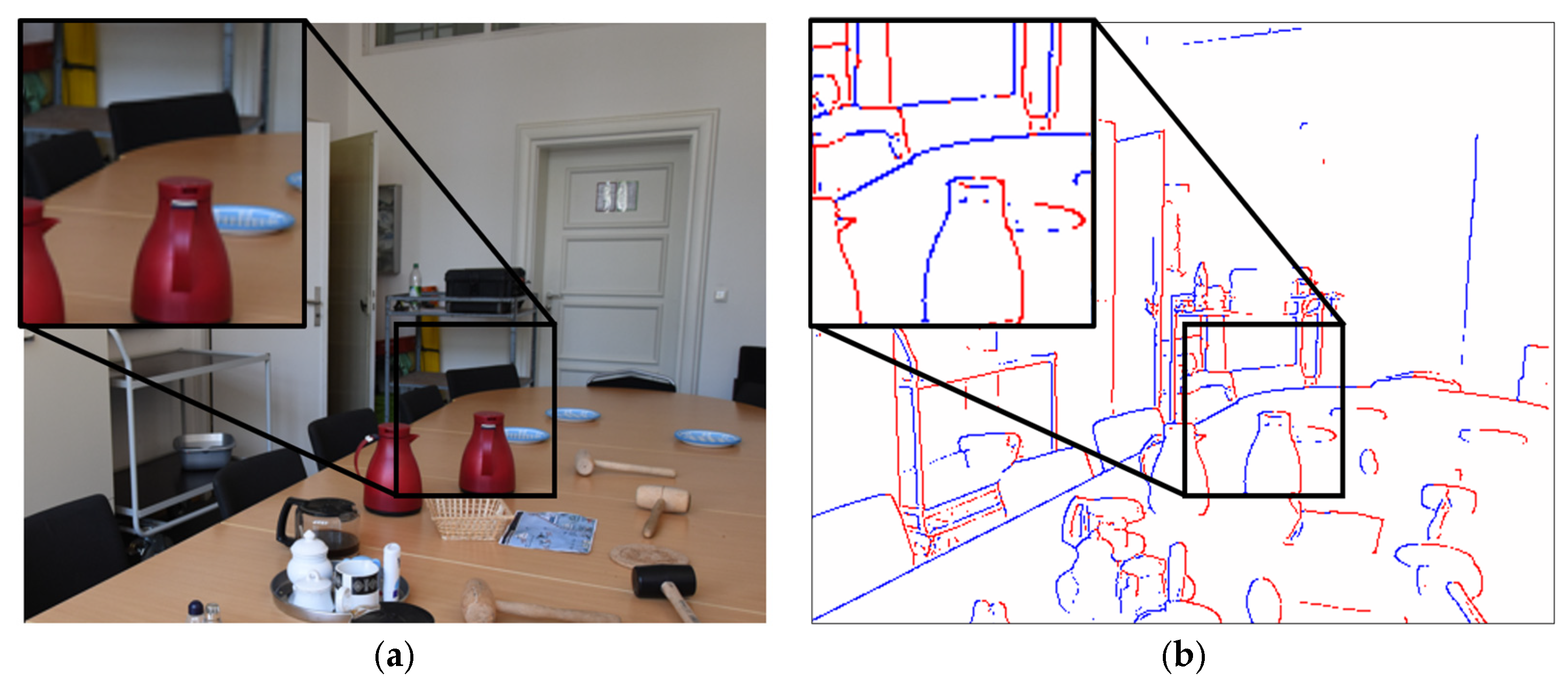
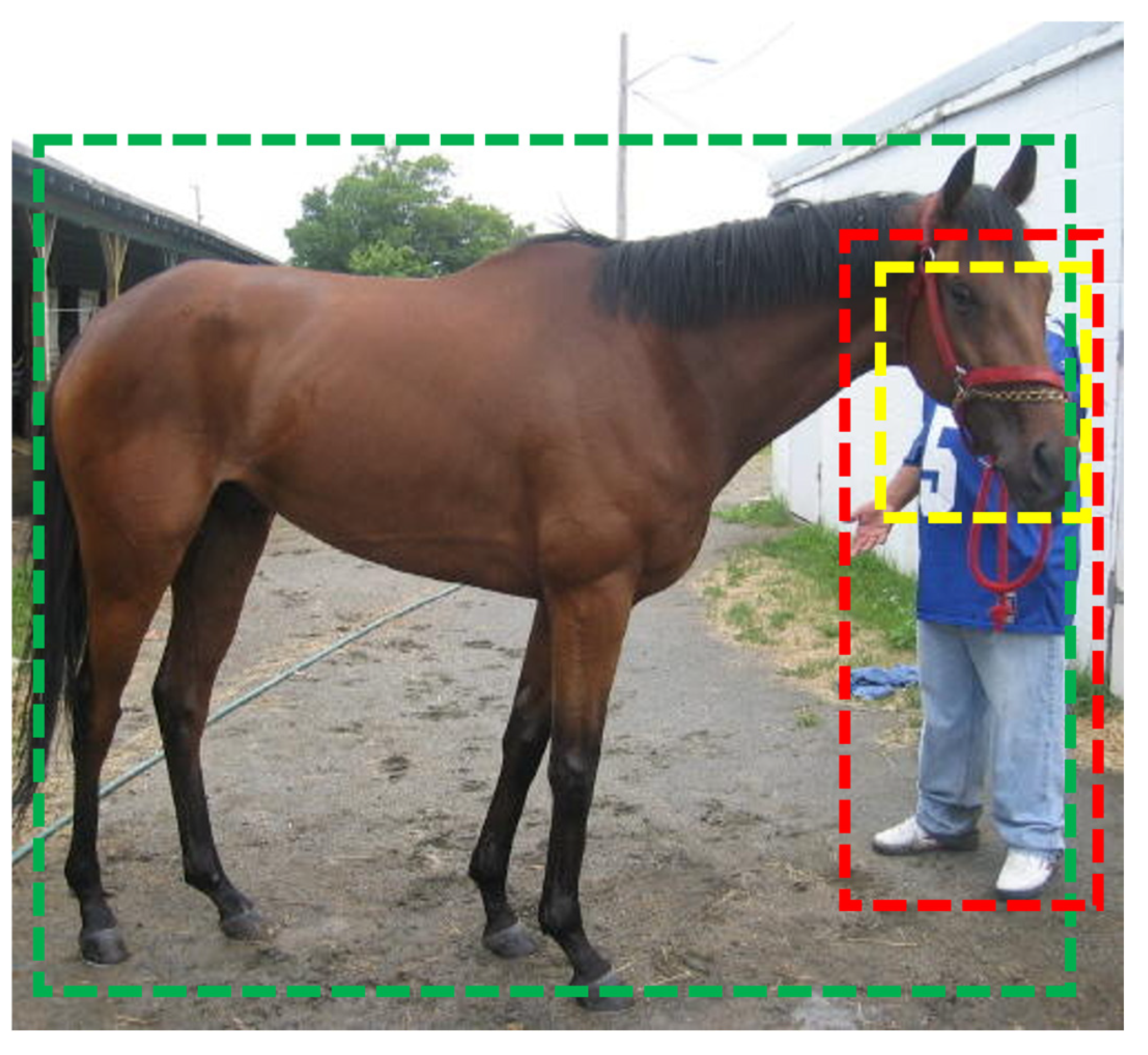
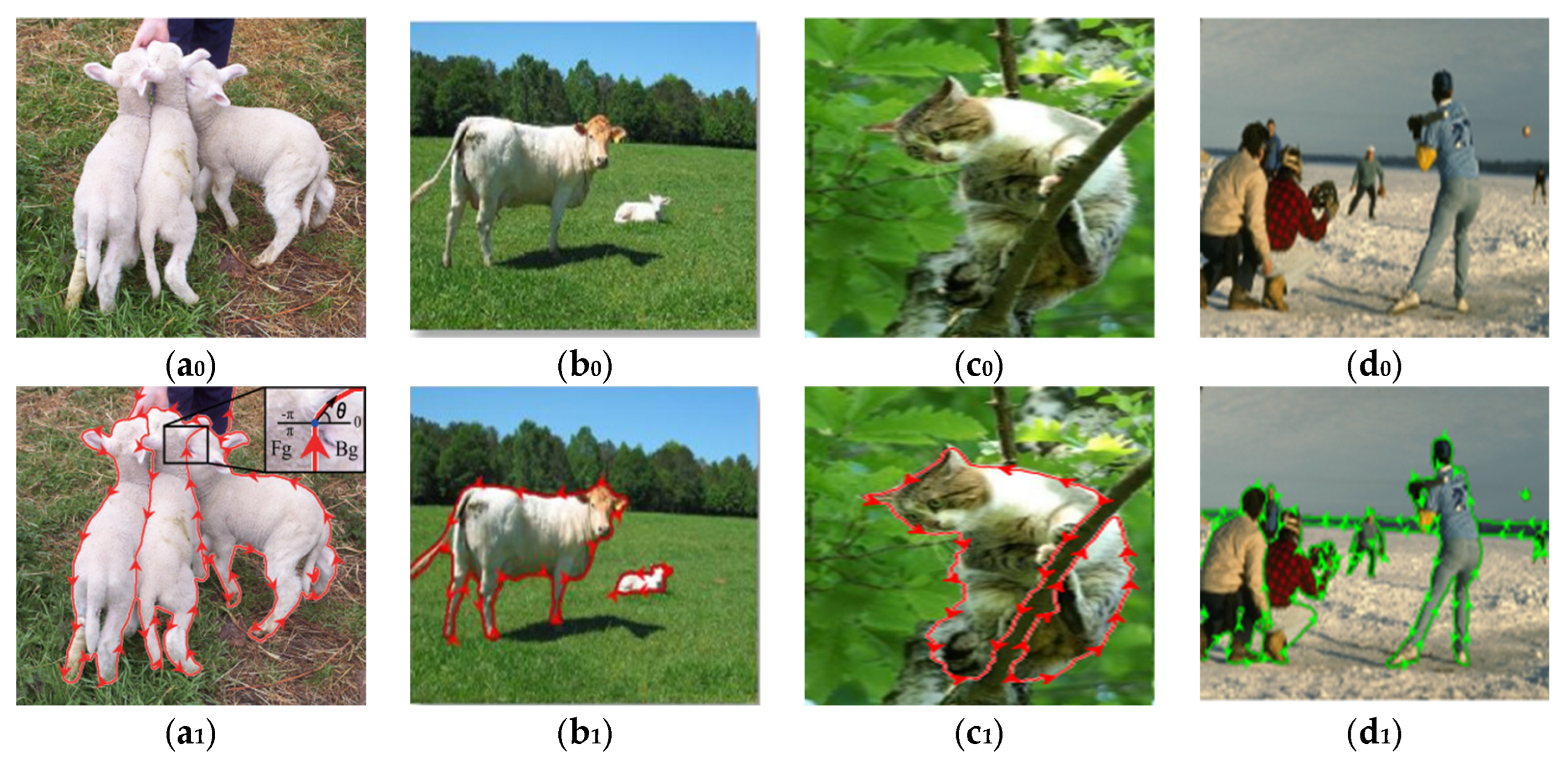
2. Occlusion Relationship Between Objects in an Image

Occlusion, in particular, is one of the most common spatial patterns in various image scenes. As shown in Figure 3, we present four major scenarios in the field of visual detection: urban street views, indoor environments, natural scenes, and crowded scenes. The regions where occlusion occurs are marked with red boxes. It can be observed that in each scenario, the probability of occlusion between objects accounts for more than 50% of the total number of objects, and, in some cases, up to 65%.

Although the occlusion spatial patterns in an image are very rich, all occlusions typically involve three key elements: the occluder, the occluded object, and the location of the occlusion. As illustrated in Figure 4, the green box highlights the occluder (“horse”), the red box shows the occluded object (“person”), and the yellow box indicates the location where the occlusion occurs. Current studies focus on pixel-level detection, or, in other words, the edges of the overlapped region between objects or between objects and the background [18,19,20,21]. As illustrated in Figure 5 (adapted from [18,19,20,21]), Figure 5a₁ presents the edge occlusion detection results of DOOBNet applied to Figure 5a₀ [18]. Similarly, Figure 5b₁ demonstrates the edge occlusion detection results of OPNet applied to Figure 5b₀ [19]. Figure 5c₁ shows the edge occlusion detection outcomes of the MT-ORL method applied to Figure 5c₀ [20], while Figure 5d₁ displays the results of the P2ORM method applied to Figure 5d₀ [21]. These network architectures primarily focus on extracting local edge patterns and pixel-level information, which is valuable but inherently limited in scope. They detect occlusion boundaries without capturing the richer semantic relationships between identified objects. Beyond these edge detection approaches, a more comprehensive understanding of occlusion requires high-level semantic features that identify the complete occlusion relationship between objects—specifically, the intra-relational structure, which is defined by three elements: the subject (the occluder), the object (the occluded entity), and occlusion (the location of occlusion). Put more directly, occlusion relationship detection is required not merely to match object detection in target identification but to uniquely accomplish what object detection fundamentally cannot achieve—the precise determination of “what occludes what” and “where occlusion occurs”.

To detect the occlusion relationship between two objects, this paper investigates two critical aspects of the problem: the detection of targets and occlusion and the matching of the subject, the object, and occlusion. Actually, this detection challenge can be addressed through a recognition process utilizing various effective object detection algorithms, such as CenterNet [16], CornerNet [11], YOLO, etc. While these algorithms can effectively locate occlusion positions and targets, they are limited in their ability to differentiate between the subject and the object and their ability to establish a relationship among the occlusion, the subject, and the object. To overcome the inherent limitations of these detection frameworks, it is essential for the detection algorithm to have the ability to detect spatial correlations of elements. Specifically, the algorithm can generate a triple list of elements that delineates the positions of the subject, the object, and occlusion, along with the corresponding confidence levels for each element and the occlusion rate (the proportion of objects that are obstructed) in an image. For the reader’s convenience, we denote the triple list as a set of the vectors

$$\begin{array}{l}O=\{<\mathrm{Sub} A_1\text{-conf, Obj} B_1\text{-conf, Occ-conf-occ rate},\dots , \\ \hspace{1em}\hspace{1em} <\mathrm{Sub} A_{\mathrm{n}}\text{-conf, Obj} B_{\mathrm{m}}\text{-conf, Occ-conf-occ rate}>\}\end{array}$$

(1)

where Sub A_i, i = 1, 2, …, n and Obj B_j, j = 1, 2, …, m are the subjects and the corresponding objects in the image, conf means the corresponding confidence level, and Occ-conf and occ rate denote the confidence level and the occlusion rate of the occlusion relationship between the specific subject and the object.

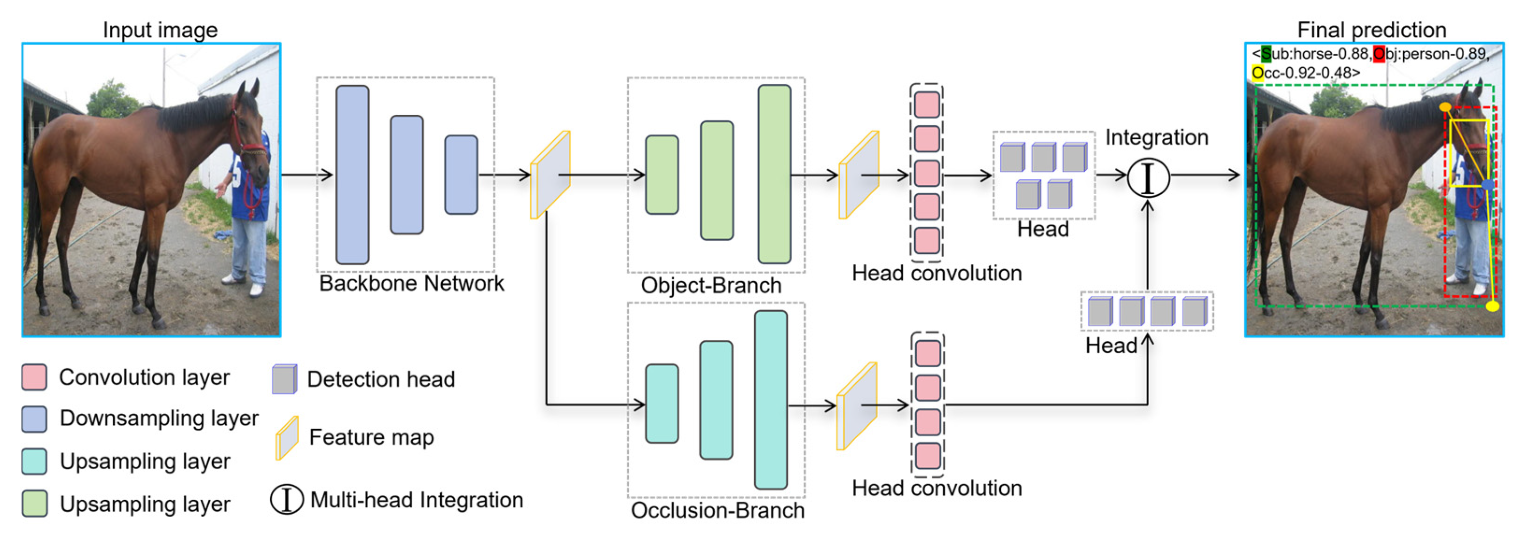
3. Deep Object Occlusion Relationship Detection Framework Design

In order to achieve a comprehensive extraction of the triple list through a deep neural network, we propose a novel occlusion relationship detection framework called DOORD-AEC. As illustrated in Figure 6, it is a two-branch (Target Branch and Occlusion Branch) end-to-end deep neural network architecture specifically designed for detecting occlusion relationships. Our goal is to use DOORD-AEC to construct an occlusion relationship graph from a set of pixels. In particular, we want to construct a keypoint graph grounded in the space of these pixels. A keypoint in this case can refer to any object of interest in the scene, including “pedestrains”, “cars”, “trunks”, “trams”, and even “occlusion”. Each occlusion keypoint is clustered together with its corresponding subject keypoint and object keypoint using associative embedding, forming a triplet representing a grouped occlusion relationship.

The framework pipeline of the DOORD-AEC can be summarized as follows. First, a backbone network processes the input image through multiple convolutional and max pooling layers to generate a global feature map. Subsequently, the feature map is fed into two parallel branches. (1) The Object Branch utilizes up-sampling layers to expand the width and height of the feature map, which is responsible for detecting object keypoints and their categories, while simultaneously predicting embedding vectors for each object, which serve as the subjects and objects in occlusion relationships. (2) The Occlusion Branch similarly processes the feature map through up-sampling layers, specifically predicting occlusion keypoints and their corresponding occlusion embedding vectors. Following this, the outputs from both branches undergo processing through their respective head convolution layers to generate detection heads. Finally, through the multi-head integration mechanism, the DOORD-AEC integrates the subject, object, and occlusion keypoints along with the clustering information predicted by the embedding vector detection heads, outputting occlusion relationships in the form of triplets <Subject-confidence, Object-confidence, Occlusion-confidence-Occlusion rate>, thereby completing occlusion relationship prediction.

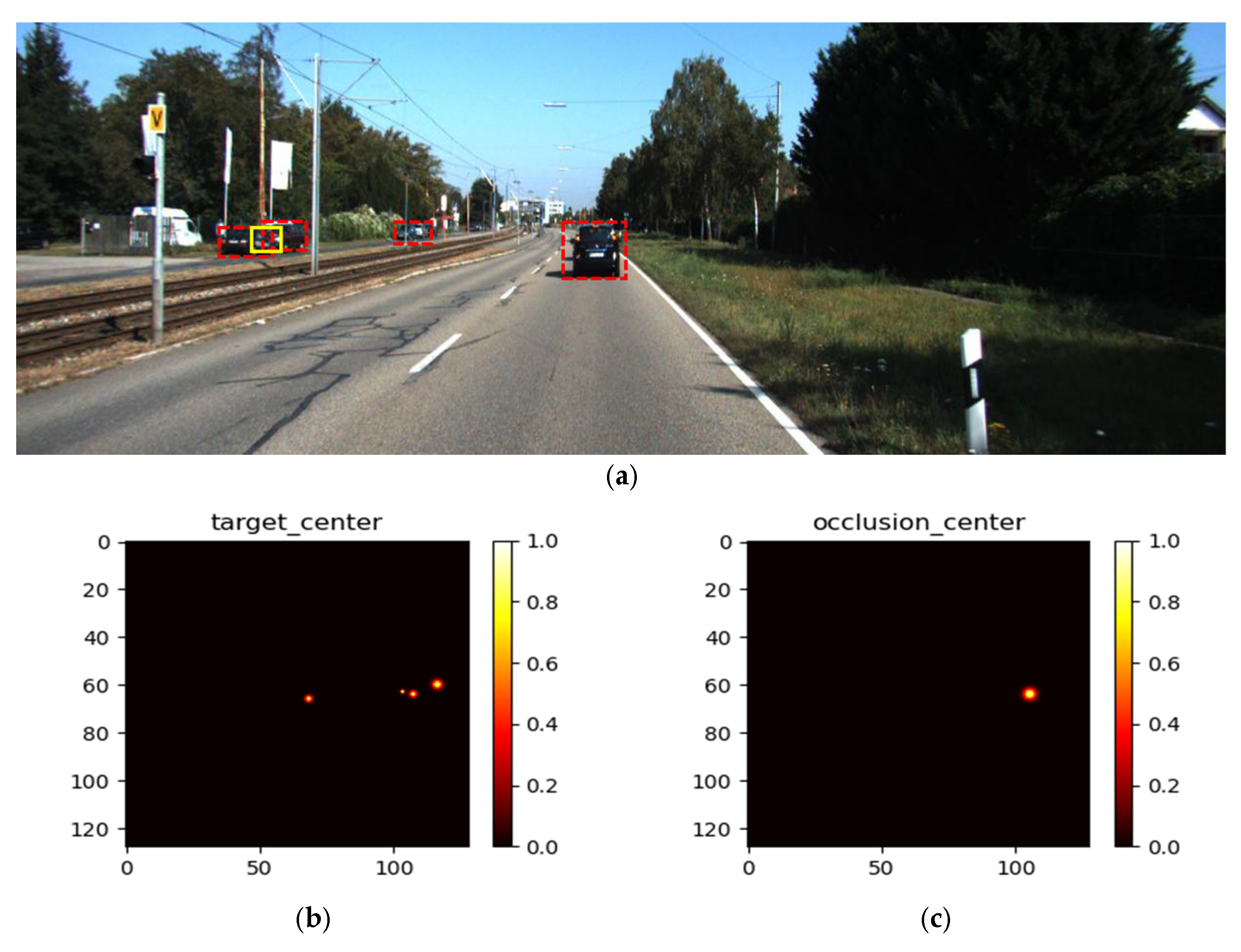
3.1. Detecting Occlusion Relationship Elements

Initially, the occlusion relationship detection framework must identify all constituents of the occlusion relationship triplet, encompassing the targets (subject and object) and occlusion. Each triplet element is grounded at a pixel location, which the network must identify. Therefore, we follow the idea of keypoint detection to detect the positions of all of the elements (targets and occlusions) in the image without considering their correlations. Keypoint detection [31,32,33] is often used in posture estimation and object detection, e.g., Openpose [34] detects the central keypoint of each joint in the human body, CenterNet [16] detects the center keypoint of the object, CornerNet [11] detects the top left corners and bottom right corners of the object, and Keypoint-Triplets detects the keypoint of the center, top left, and bottom right.

Concretely, let I ∈ R^W×H×3 represent an input image of width W and height H. Our aim is to produce an element heatmap of two branches (the Object Branch and the Occlusion Branch), $\widehat{Y}=\{{\widehat{Y}}_T\in {\left[0, 1\right]}^{{\displaystyle \frac{W}{R}}\times {\displaystyle \frac{H}{R}}\times C}, {\widehat{Y}}_O\in {\left[0, 1\right]}^{{\displaystyle \frac{W}{R}}\times {\displaystyle \frac{H}{R}}\times {\mathrm{C}}^{\prime }}\}$, where ${\widehat{Y}}_T$ is the target heatmap, ${\widehat{Y}}_{\mathrm{O}}$ is the occlusion heatmap, R = 4 is the output stride, and C is the number of keypoint types. In our case, ${\mathrm{C}}^{\prime }=1$ denotes the occlusion and C = 7 denotes the categories of targets, which include “car”, “van”, “truck”, “pedestrian”, “person sitting”, “cyclist”, and “tram”. A prediction ${\widehat{Y}}_{T\left(x,y,c\right)}=1$ corresponds to detected target, ${\widehat{Y}}_{O\left(x,y,c^{\prime }\right)}=1$ corresponds to detected occlusion, while ${\widehat{Y}}_{T\left(x,y,c\right)}=0$ is the background other than the target and ${\widehat{Y}}_{O\left(x,y,c^{\prime }\right)}=0$ is the background other than the occlusion.

Accurately predicting an element from a single pixel in the heatmaps $\widehat{Y}$ poses significant challenges. Therefore, our objective is to generate a Gaussian distribution centered at the detected element’s location within $\widehat{Y}$, thereby enhancing the heatmap’s features for element localization. Let C_t = (C_tx, C_ty) denote the coordinates of the element’s center point in $\widehat{Y}$. The Gaussian distribution around C_t can be obtained as follows:

$$E_c(x,y)=\mathit{exp}(-{\displaystyle \frac{{(x-C_{\mathit{tx}})}^2+(y-C_{\mathit{ty}}{)}^2}{2{\mathsf{\sigma }}_p^2}})$$

(2)

where (x, y) denotes the coordinate of the pixel in the heatmap, ${\sigma }_p$ is an element size-adaptive standard deviation, and the subscript C denotes the channel of the Gaussian kernel, with $E_c$ corresponding to c-th channel associated with the keypoint’s class. The parameter ${\sigma }_p$ ensures that the radius of the Gaussian distribution is proportional to the element size, typically ${\sigma }_p$, which can be set to 1/3 of the element size. We generate ground-truth $Y=\{Y_T\in {\left[0, 1\right]}^{{\displaystyle \frac{W}{R}}\times {\displaystyle \frac{H}{R}}\times C},Y_O\in {\left[0, 1\right]}^{{\displaystyle \frac{W}{R}}\times {\displaystyle \frac{H}{R}}\times C^{\prime }}\}$ heatmaps by placing Gaussian distribution at each annotated element center. Y_T contains Gaussian distributions centered at all object elements, while Y_O contains Gaussian distributions centered at all occluded elements. Both heatmaps are constructed based on Equation (1), ensuring a consistent representation approach across visible targets and occlusions. This is shown in Figure 7, where the targets in image I are marked with red dashed boxes and the occlusion is marked with yellow implementation boxes. Figure 7b illustrates the Gaussian distribution of the target elements’ positions on heatmap Y_T, while the Gaussian distribution of the occlusion elements’ positions on heatmap Y_O is also depicted in Figure 7c.

Let ${\widehat{Y}}_{x,y,c}$ be the score at location (x, y) for class c of the element in the predicted heatmaps Y, and let Y_x,y,c be the ground-truth heatmap augmented with the unnormalized Gaussian distribution. The training objective is a penalty-reduced pixelwise logistic regression with focal loss, following CenterNet [16] and CornerNet [11]:

$$L_E={\displaystyle \frac{-1}{N}}{\displaystyle \sum _{x,y,c}\left\{\begin{array}{ll}{(1-{\widehat{Y}}_{x,y,c})}^{\alpha }\log ({\widehat{Y}}_{x,y,c}),& \mathrm{if} Y_{x,y,c}=1\\ {(1-Y_{x,y,c})}^{\beta }{({\widehat{Y}}_{x,y,c})}^{\beta }\log (1-{\widehat{Y}}_{x,y,c}),& \mathrm{otherwise}\end{array}\right.}$$

(3)

where α and β are hyper-parameters of the focal loss, α = 2 and β = 4 in our experiments. N is the number of keypoints of the element in image I. x, y, and c denote the x-axis, the y-axis, and the channel in the heatmap of the pixel, respectively. Additionally, to achieve accurate localization of all elements within a triplet, it is necessary to regress the width and height $\widehat{D}=\{{\widehat{D}}_T\in {\Re }^{{\displaystyle \frac{W}{R}}\times {\displaystyle \frac{H}{R}}\times 2}, {\widehat{D}}_O\in {\Re }^{{\displaystyle \frac{W}{R}}\times {\displaystyle \frac{H}{R}}\times 2}\}$ of the elements, where ${\widehat{D}}_T$ is the width and height of the target element and ${\widehat{D}}_O$ is the width and height of the occlusion element. Utilize the Mean Absolute Error (MAE) loss,

$$L_{wh}={\displaystyle \sum _{i\in \left\{w,h\right\}}\left\{\begin{array}{ll}0.5\times {\left(D_i-{\widehat{D}}_i\right)}^2,& \mathrm{if} \left|D_i-{\widehat{D}}_i\right|<1\\ \left|D_i-{\widehat{D}}_i\right|-0.5,& \mathrm{otherwise}\end{array}\right.}$$

(4)

where D denotes the ground-truth of the feature map with the width and height of the element and w and h represent the channel with the element’s width and height. To compensate for the quantization error that occurs during convolution when discretizing continuous coordinates into integer grid positions in the heatmap, we also need to predict the offset $\widehat{O}=\{{\widehat{O}}_T\in {\Re }^{{\displaystyle \frac{W}{R}}\times {\displaystyle \frac{H}{R}}\times 2}, {\widehat{O}}_O\in {\Re }^{{\displaystyle \frac{W}{R}}\times {\displaystyle \frac{H}{R}}\times 2}\}$ for each element. We similarly utilize the MAE loss to supervise the regression of all elements’ planar positions, as depicted by the following equation:

$$L_{off}={\displaystyle \sum _{i\in \left\{x,y\right\}}\left\{\begin{array}{ll}0.5\times {\left(O_i-{\widehat{O}}_i\right)}^2,& \mathrm{if} \left|O_i-{\widehat{O}}_i\right|<1\\ \left|O_i-{\widehat{O}}_i\right|-0.5,& \mathrm{otherwise}\end{array}\right.}$$

(5)

where O denotes the ground-truth of the feature map with local offset of the element and x and y represent the horizontal offset channel and the vertical offset channel of the element, respectively. The supervision acts only at keypoint locations of the element, and all other locations are ignored.

3.2. Grouping Occlusion Relationship Elements with Associative Embedding Clustering

Next, the occlusion needs to be put together with its subject and object, that is, we need to cluster a set of occlusion relationships of the subject, object, and occlusion elements together. We introduce a novel associative embedding-based clustering method, referred to as AE-Clustering. AE-Clustering aims to partition two sets of elements. Target set T = {t₁, t₂,…,t_n} and occlusion set O = {o₁, o₂,…,o_m} into m + 1 clusters using AEC = {C₁,C₂,…,C_m,C_m+1} representation, where $C_k=\left\{t_i,t_j,o_k\left|k\in \left[1,m\right],i,j\right.\in \left[1,n\right],i\ne j\right\}$ represents the set of all occlusion triplets (subject, object, and occlusion) and $C_{m+1}=\left\{t_p\left|p\in \left[1,n\right],p\ne i,p\ne j\right.\right\}$ represents the target without occlusion. Figure 8 shows a step by step decomposition of the AE-Clustering algorithm. In Figure 8a, the five-pointed star represents occlusion set O, and the gray dot represents target set T. C_k represents the k subgroups of the cluster, which includes an occlusion along with its corresponding subject and object targets. AE-Means assigns a random numerical embedding value to each cluster center and the cluster members. Subsequently, AE-Clustering obtains cluster members corresponding to each cluster center based on ground-truth, as well as the remaining target members that do not require clustering. In Figure 8b, the cluster centers and cluster members are marked with the same color. Next, AE-Clustering uses “push” and “pull” actions (shown in Figure 8c) to minimize the difference in associative embedding values AE between cluster members (targets) that match the cluster center (occlusion). AE is obtained as follows:

$$AE={\displaystyle {\displaystyle \sum _{k=1}^m}{\displaystyle \sum _{t_i\in C_k}{‖e\left(t_i\right)-e\left(o_k\right)‖}^2}}+{\displaystyle {\displaystyle \sum _{k=1}^m}{\displaystyle \sum _{t_i\notin C_k}\max \left(0,\delta -{‖e\left(o_k\right)-e\left(t_i\right)‖}^2\right)}}+{\displaystyle {\displaystyle \sum _{k=1}^m}{\displaystyle {\displaystyle \sum _{k^{\prime }\ne k}}\max \left(0,\delta -{‖e\left(o_k\right)-e\left(o_{k^{\prime }}\right)‖}^2\right)}}$$

(6)

where e(t_i) represents the embedding value of target element t_i, e(o_k) represents the embedding value of occlusion element o_k, and δ is a margin parameter to ensure sufficient separation.

It is important to note that the AE-Clustering process typically requires multiple iterations for completion. The “push” and “pull” operations are performed repeatedly, with embedding values being updated in each iteration until the clustering converges to a stable state, thereby grouping elements with occlusion relationships into a cluster. Figure 8d presents a visualization of the completed AE-Clustering results, where each cluster C_k is identified with a distinct color. The gray dots represent targets that do not require clustering, indicating that these elements are not part of any occlusion spatial relationship.

In our case, as discussed in Section 3.1, all occlusion elements and target elements have already been detected, meaning AE-Clustering step 1 is already in place. AE-Clustering step 2, which determines all cluster centers and corresponding cluster members, can be fully obtained based on the ground-truth of occlusion relationships. Then, by training the network to produce additional outputs in the two branches of element detection and using loss functions as constraints (AE-Clustering step 3), AE-Clustering (AE-Clustering step 4) becomes possible. For every cluster member (target), the network produces two different identifiers in the form of vector embedding [35], with one representing the subject (foreground embedding) and one representing the object (background embedding). The subject is the occluded foreground target, and the object is the occluded background target. For every cluster center (occlusion), it must produce the corresponding embeddings (occlusion embedding) to refer to its cluster members (the subject and the object). The network must learn to ensure that the embedding distances between subjects, objects, and occlusions in the same cluster are small and that the embedding distances between elements in different clusters are big. The actual values of the embeddings are unimportant [36,37]. Only the distances between the embeddings are used to cluster the target and occlusion.

We follow the corner embeddings of CornerNet [11] and pixels to graphs through associative embedding of thought and use embeddings of 1 dimension. In the Object Branch, additional foreground embedding detection head $\widehat{P}\in {\Re }^{{\displaystyle \frac{W}{R}}\times {\displaystyle \frac{H}{R}}\times 1}$ and background embedding detection head $\widehat{B}\in {\Re }^{{\displaystyle \frac{W}{R}}\times {\displaystyle \frac{H}{R}}\times 1}$ are the output, and, in the Occlusion Branch, additional occlusion embedding detection head $\widehat{C}\in {\Re }^{{\displaystyle \frac{W}{R}}\times {\displaystyle \frac{H}{R}}\times 1}$ is the output. We think of the network’s “pull together” as a cluster, that is, a triplet of the subject, the object, and occlusion, and of “pushing apart” as another cluster, that is, a triplet of elements. Let f_k be the foreground embedding for the target k in $\widehat{P}$, b_k be the background embedding for the target k in $\widehat{B}$, and e_k be the occlusion embedding in their group in $\widehat{C}$. Given an image with M cluster center (occlusions), the loss to “pull together” these embeddings is, in training,

$$L_{pull}={\displaystyle \frac{1}{M}}{\displaystyle {\displaystyle \sum _{k=1}^M}\left[{\left(e_k-f_k\right)}^2+{\left(e_k-b_k\right)}^2\right]}$$

(7)

To “push apart” embeddings across different clusters, we merely used a strategy of “pushing apart” the cluster center (occlusions) from each other:

$$L_{push}={\displaystyle \frac{1}{M(M-1)}}{\displaystyle {\displaystyle \sum _{k=1}^M}{\displaystyle {\displaystyle \sum _{\begin{array}{l}j=1\\ j\ne k\end{array}}^M}\max \left(0,\mathsf{\Delta }-{\left(e_k-e_j\right)}^2\right)}}$$

(8)

where M is the number of the cluster center (occlusion) and $\mathsf{\Delta }$ is 8 in all of our experiments. Similarly to the offset loss, we only apply the losses at the ground-truth element’s location.

3.3. Multi-Head Integration

The multi-head integration process combines predictions from different detection heads to produce the final output. Specifically, confidence thresholding is applied to keep only the high-confidence object and occlusion centers in ${\widehat{Y}}_T$ and ${\widehat{Y}}_O$, and we set the threshold to 0.5. Next, bounding boxes are generated and remapped to the original image size, followed by NMS (Non-Maximum Suppression) [8,12]. Then, obtain the occlusion embedding set S_o = {eocc₁, eocc₂, eocc₃, …, eocc_w} for w occlusion keypoint from $\widehat{C}$, obtain the foreground embedding set S_p = {efor₁, efor₂, efor₃, …, efor_m} for m subject keypoint from $\widehat{P}$, and obtain the background embedding set S_b = {ebac₁, ebac₂, ebac₃, …, ebac_m} for m object keypoint from $\widehat{B}$. For each occlusion, find the target with the smallest distance on the foreground embedding output $\widehat{P}$ as its subject, and find the target with the smallest distance on the background embedding $\widehat{B}$ as its object, thus forming a triplet of occlusion relationships among the three primary groups, as outlined in Algorithm 1.

Algorithm 1 DOORD-AEC inference algorithm

Input: Image I

Output: Triplet set of occlusion relationship

1: Image I pass through DOORD-AECNet

2: Position all elements (occlusion, subject and object)

3: Get set So, Sp and Sb from detected elements

4: for i = 1, 2, …, w do

5:  Get eocci from So

6:  for j = 1, 2, …, m do

7:    Get Sij= (eocci − eforj)2 and Oij = (eocci − ebacj)2

8:   end for

9:   Get the set of distance Ds = {Si0, Si1, …, Sim} with subject, get the set of distance Do = {Oi0, Oi1, …,Oim}

10:   Get subject and object through the index Index(Min(Ds)) and Index(Min(Do))

11:   Get a triplet of occlusion relationship

12: Get triplet set of all the occlusion relationship

13: end for

Additionally, in the occlusion relationship triplet, the occlusion rate is also considered, which represents the proportion of the object area occluded by the subject. After completing the localization and regression calculations for the various elements, the occlusion percentage R is computed using the following formula:

$$R={\displaystyle \frac{\mathrm{Area}\left(Occ\cap Obj\right)}{\mathrm{Area}\left(Obj\right)}}$$

(9)

where Occ is the area of the detected occlusion and Obj is the area of the detected object.

3.4. Architecture of DOORD-AECNet

We provide all details of the DOORD-AECNet structure in

Table 1. Network architecture specification of our DOORD-AECNet.

Stage	Layer Name	Size (in/out)	Channels (in → out)	Layer Type	Activation	Note
Input	input	512 × 512 512 × 512	3 → 3	-	-	Input image
Backbone	Conv1	512 × 512 256 × 256	3 → 64	[7 × 7, 64], stride = 2, padding = 3	ReLU + BN
	Maxpool	256 × 256 128 × 128	64 → 64	Maxpool 3 × 3, stride = 2, padding = 1	-	-
	Stage 1	128 × 128 128 × 128	64 → 256	[1 × 1, 64] [3 × 3, 64] [1 × 1, 256] × 3 stride = 1, padding = 1	ReLU + BN	Skip connection
	Stage 2	128 × 128 64 × 64	256 → 512	[1 × 1, 128] [3 × 3, 128] [1 × 1, 512] × 4 stride = 2, padding = 1	ReLU + BN	Skip connection
	Stage 3	64 × 64 32 × 32	512 → 1024	[1 × 1, 256] [3 × 3, 256] [1 × 1, 1024] × 23 stride = 2, padding = 1	ReLU + BN	Skip connection
	Stage 4	32 × 32 16 × 16	1024 → 2048	[1 × 1, 512] [3 × 3, 512] [1 × 1, 2048] × 3 stride = 2, padding = 1	ReLU + BN	Skip connection
Object Branch	Upconv1_1	16 × 16 32 × 32	2048 → 256	[3 × 3, 256], stride = 1, padding = 1 [4 × 4, 256]^T, stride = 2, padding = 1	ReLU + BN	Fed by “stage 4”
	Upconv1_2	32 × 32 64 × 64	256 → 128	[3 × 3, 128], stride = 1, padding = 1 [4 × 4, 128]^T, stride = 2, padding = 1	ReLU + BN	Fed by “Upconv1_1”
	Upconv1_3	64 × 64 128 × 128	128 → 64	[3 × 3, 128], stride = 1, padding = 1 [4 × 4, 64]^T, stride = 2, padding = 1	ReLU + BN	Fed by “Upconv1_2”
Occlusion Branch	Upconv2_1	16 × 16 32 × 32	2048 → 256	[3 × 3, 256], stride = 1, padding = 1 [4 × 4, 256]^T, stride = 2, padding = 1	ReLU + BN	Fed by “stage 4”
	Upconv2_2	32 × 32 64 × 64	256 → 128	[3 × 3, 128], stride = 1, padding = 1 [4 × 4, 128]^T, stride = 2, padding = 1	ReLU + BN	Fed by “Upconv2_1”
	Upconv2_3	64 × 64 128 × 128	128 → 64	[3 × 3, 128], stride = 1, padding = 1 [4 × 4, 64]^T, stride = 2, padding = 1	ReLU + BN	Fed by “Upconv2_2”
Head Convolution	Target_cen	128 × 128 128 × 128	64 → 7	[3 × 3, 64] stride = 1, padding = 1 [3 × 3, 7] stride = 1	ReLU + BN	Fed by “Upconv1_3”
	Target_wh	128 × 128 128 × 128	64 → 2	[3 × 3, 64] stride = 1, padding = 1 [3 × 3, 2] stride = 1	ReLU	Fed by “Upconv1_3”
	Target_off	128 × 128 128 × 128	64 → 2	[3 × 3, 64] stride = 1, padding = 1 [3 × 3, 2] stride = 1	ReLU	Fed by “Upconv1_3”
	Sub_emb	128 × 128 128 × 128	64 → 1	[3 × 3, 64] stride = 1, padding = 1 [3 × 3, 1] stride = 1	ReLU	Fed by “Upconv1_3”
	Obj_emb	128 × 128 128 × 128	64 → 1	[3 × 3, 64] stride = 1, padding = 1 [3 × 3, 1] stride = 1	ReLU	Fed by “Upconv1_3”
	Occlusion_cen	128 × 128 128 × 128	64 → 1	[3 × 3, 64] stride = 1, padding = 1 [3 × 3, 1] stride = 1	ReLU + Sigmoid	Fed by “Upconv2_3”
	Occlusion_wh	128 × 128 128 × 128	64 → 2	[3 × 3, 64] stride = 1, padding = 1 [3 × 3, 2] stride = 1	ReLU	Fed by “Upconv2_3”
	Occlusion_off	128 × 128 128 × 128	64 → 2	[3 × 3, 64] stride = 1, padding = 1 [3 × 3, 2] stride = 1	ReLU	Fed by “Upconv2_3”
	Occ_emb	128 × 128 128 × 128	64 → 1	[3 × 3, 64] stride = 1, padding = 1 [3 × 3, 1] stride = 1	ReLU	Fed by “Upconv2_3”
Integration	-	-	-	-	-	Multi-head integration

[k × k, c]: denotes c convolutional filters of size k × k. [k × k, c] ^T: denotes c transposed convolutional filters of size k × k. BN denotes Batch Normalization. → denotes channel transformation, where the left side represents the number of channels in input feature maps and the right side shows the number of channels in output feature maps.

. DOORD-AECNet is a two-branch, fully convolutional network that expands upon the hourglass structure by adding an up-sampling branch to create a cloverleaf-shaped architecture [11,16,38,39,40,41,42]. This design establishes a clear semantic division of labor between the two branches—one branch is dedicated to object detection, while the other specializes in occlusion detection. These represent fundamentally different semantic tasks that require distinct feature extraction capabilities. By separating these responsibilities into dedicated pathways, the network can simultaneously optimize for both objectives without forcing a single branch to handle competing semantic concepts. This separation enables DOORD-AECNet to maintain high performance in complex scenarios where objects may be partially obscured, as each branch can focus on its specialized semantic role without compromising the other’s effectiveness.

Specifically, the first part is designed for feature extraction, which can be configured using any effective deep neural network model, such as VGG [3], ResNet [5], InceptionNet [4], and DenseNet [43]. In our implementation, we adopt ResNext101, which has been pre-trained for image classification. For the feature extraction phase, the input color image (512 × 512 size) is highly compressed into latent features through a series of deeply stacked convolutional blocks. As a result, the spatial dimensions of these features are reduced to 1/32 of the original resolution, while the number of channels remains substantial.

The second part consists of two parallel up-sampling branches, the Object Branch and the Occlusion Branch. They enhance a standard residual network by incorporating three up-convolutional networks, thereby facilitating a higher-resolution output. This up-convolutional phase ensures that the output size of the heatmap (128 × 128 pixels) is adequate to meet the coding requirements for the element center point region and the embeddings.

The third part is the detection head section. The output of Object Branch employs five parallel pathways with two consecutive convolutional layers each, resulting in the output of five detection heads. The first head is an N-channels heatmap, which has a Gaussian distribution at the center keypoint of targets. Each channel of the heatmap corresponds to a category of the target. The second head is a two-channel feature map that predicts the width and height. The third head is responsible for fine-tuning the flat position of the targets keypoints. The fourth and fifth detection heads are both single-channel and individually predict target keypoints as embeddings for the subject (the foreground target) and the object (the background target), respectively. Similarly, the output of the Occlusion Branch utilizes four parallel pathways with two consecutive convolutional layers each to yield four detection heads. These heads are responsible for detecting the center point of the occlusion and the width and height of occlusions, as well as embedding of the occlusion.

4. Experiments and Analysis

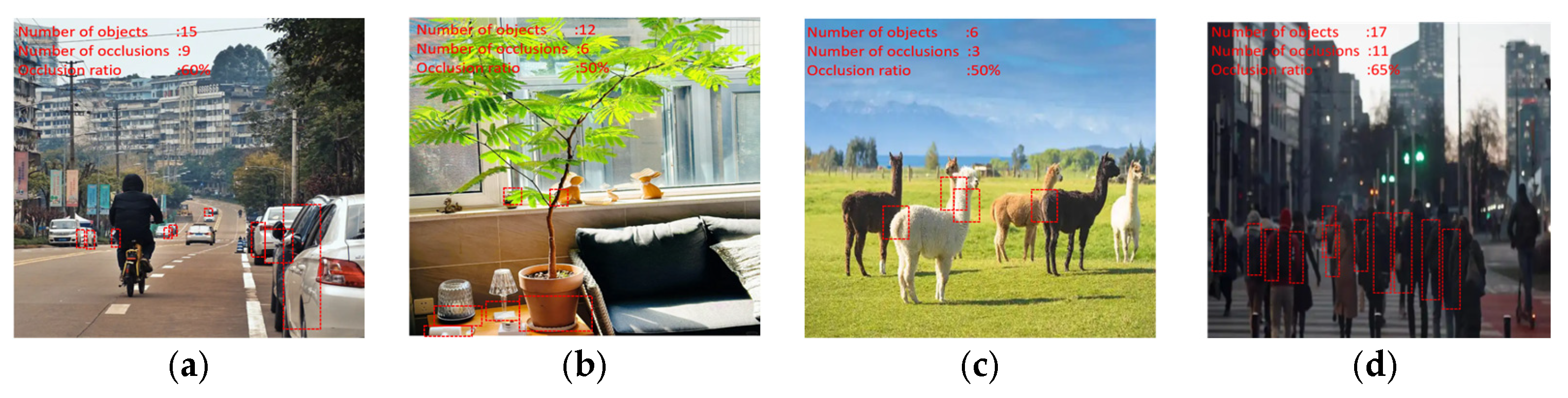
4.1. Dataset and Experimental Setup

Because a large dataset is critical for training and evaluating deep network models, we chose to annotate occlusion relationships using the Karlsruhe Institute of Technology and Toyota Technological Institute at Chicago (KITTI) Vision Benchmark Suite because it contains well-selected images [30]. And, other researchers have already annotated the boundaries, dimensions, depths, etc. for 8 object instances. We annotated occlusion positions between objects based on existing publicly available data. Each occlusion position was delineated using bounding boxes by specifying the foreground subject and the background object of the occlusion box, which was ultimately represented as a triplet (subject, occlusion, object). As depicted in Figure 9, the blue shaded box represents the annotated occlusion region, with the red box indicating the primary subject of the occlusion relationship and the green box representing the secondary object of the occlusion relationship. Using the above method, we have developed a novel occlusion relationship dataset named the KITTI Occlusion Relationship Dataset (KORD).

Our KORD contains 7481 images with 7 object categories (car, van, truck, pedestrian, person sitting, cyclist, tram) and 14,462 occlusions. Among these instances, there are 14,462 occurrences of a car occluding another car, 1733 instances where a van occludes a car, 1128 cases where a pedestrian occludes another pedestrian, and 840 occurrences where a car occludes a van. Additionally, there are 377 instances where a truck occludes a car. Furthermore, there are a total of 2294 occlusion instances involving various other types of objects. Figure 10 shows a statistical graph of the number of occlusions that occur between different subjects and objects. We use 6733 images in our training set and test the remaining 783 images.

Experiment Environment: Experimental training and testing were performed using a HASEE laptop. The system is Win10, equipped with an inter-i5-11400 CPU and an NVIDIA GeForce RTX 3070 laptop GPU. The video memory size is 8 GB. The running environment of the experiment is Python 3.8, Pytorch 1.7.0, Cuda11.1 parallel computing architecture, and the Cudnn8.04 neural network accelerator library.

4.2. Model Training

In this paper, a deep convolutional neural network called DOORD-AECNet with pre-trained ResNet [5] as the backbone was trained. The training process of this CNN model was divided into two stages, namely, the frozen stage and the thawy stage. To conserve resources and minimize training time, we began by freezing the ResNet [5] backbone feature extraction network’s weights. Then, we trained 100 epochs of unfrozen network structure parameters. Finally, all network structures were trained together for 300 epochs. During the frozen training stage, only the parameters of the latter half of the model were adjusted, resulting in smaller video memory occupancy. Thus, the batch size was set to 8 for this stage. However, in the thawy training stage, the parameters of all models began to be updated, requiring greater video memory. So, we halved the batch size during training. The Adam optimizer was employed as the model training optimizer, with the learning rate adaptively adjusted based on the loss change. The maximum learning rate was 50⁻⁴, and the minimum learning rate was 50⁻⁶.

4.3. Metric and Results

The occlusion relationship detection task is defined as the production of a set of subject–object–occlusion relationship tuples in this paper. A proposed triplet is composed of three elements, with the subject and the object defined by their class and bounding box, while occlusion is only defined by the bounding box. Most visual relationship detection algorithms are evaluated using R@K as evaluation metrics for detection in the visual relationship dataset [26,44,45]. R@K computes the fraction of times a true relationship is predicted in the top K confident relationship predictions in an image [46,47,48]. They generally believe that precision and average precision (AP) are not proper metrics, as visual relationships are labeled incompletely and will penalize the detection if they do not have that particular ground-truth in some visual relationship detection datasets. But, on the KORD dataset we introduced, each occlusion was clearly marked, indicating the foreground targets and background targets of the occlusion. So, there is no such flaw, and a more trustworthy and comprehensive AP can be used for evaluation.

The AP metric is a fundamental measure used to evaluate the performance of detection models [48,49]. To further understand the underlying performance of a model, we typically look at three fundamental metrics: precision (P), recall (R), and the F1-Score (F1). These metrics are essential in evaluating the quality of detection results. Precision measures the accuracy of positive predictions made by the model. It is the ratio of true positive detections to the total number of positive predictions. Recall measures the completeness of positive predictions made by the model. It is the ratio of true positive detections to the total number of ground-truth positives. F1 is a valuable metric for evaluating detection models, offering a holistic assessment of precision and recall performance.

$$Precision={\displaystyle \frac{TP}{TP+FP}}$$

(10)

$$Recall={\displaystyle \frac{TP}{TP+FN}}$$

(11)

$$F1={\displaystyle \frac{2\times Precision\times Recall}{Precision+Recall}}$$

(12)

where TP denotes the proportion of positive predictions that were correctly predicted, FP denotes the proportion of negative predictions that were inaccurately predicted, TN represents the proportion of negative predictions that were correctly predicted, and FN represents the proportion of incorrectly predicted positive predictions. AP is calculated by computing the area under the precision–recall curve. It summarizes the model’s ability to detect across all levels of confidence, and, the larger the AP, the better the detection effect.

In our occlusion relationship detection task, a triplet is correct if the subject and object classes match those of a ground-truth annotation and the subject, object, and occlusion have at least a T intersection over union (IOU) [49] overlap with the corresponding ground-truth. As depicted in

Table 2. Performance of occlusion relationship detection.

Task	Score_Threhold	Overlap T	F1	Recall	Precision	AP
Occlusion relationship detection	0.5	0.3	0.70	0.57	0.91	0.63
	0.5	0.4	0.68	0.55	0.89	0.60
	0.5	0.5	0.65	0.53	0.85	0.56
	0.5	0.6	0.60	0.49	0.78	0.48
	0.5	0.7	0.49	0.40	0.64	0.35

, we established a confidence threshold of Score_threhold = 0.5 to identify detected occlusions. The table enumerates the F1, recall, and precision for occlusion relationship detection across various Overlap T scales. Additionally, it presents the AP values corresponding to these thresholds. Figure 11a–c visualize the curves of F1, recall, and precision as functions of the Score_Threshold under the condition of Overlap T = 0.5. Figure 11d depicts the PR (precision–recall) curve for occlusion relationship detection at Overlap T = 0.5 with Score_threhold = 0.5.

From the various metrics in Table 2 and Figure 11, it can be seen that our occlusion relationship detection model DOORD-AECNet has achieved impressive results. Across different Overlap configurations, AP and precision performed well. However, the recall rate was slightly lower in comparison. This is expected because there are two types of occlusion scenes commonly present in the dataset. Firstly, the lower recall is due to occlusions, which are significantly smaller in size compared to the subjects and objects, making them easier to miss, as illustrated in Figure 12a. Specifically, the green bounding box represents the occlusion box, while the red box represents the target box. The occlusion box occupies only 0.2% of the image’s pixel area and is smaller than one-tenth of the size of the other target boxes. Secondly, as shown in Figure 12b, occluded scenes often involve very elongated bounding boxes (the green bounding boxes), with aspect ratios sometimes reaching 17%, making it challenging to locate occlusion positions using keypoint detection principles.

In addition to detection metrics, we also evaluated the computational efficiency of our model. On a standard NVIDIA RTX 3070 GPU, DOORD-AECNet processes a single frame in approximately 26 ms (39 FPS), making it suitable for near real-time applications. This efficiency is achieved while maintaining high detection quality.

We also show extensive qualitative results in Figure 13. Although these images have various complex natural scenes with multiple objects, our method can effectively detect both unobstructed targets and triplets with occlusion relationships simultaneously. We have outlined the detected subject and the object with dashed boxes and indicated the predicted occlusion with solid boxes. The bottom right corner of the occlusion area (purple point) is connected by a yellow line to the bottom right corner of the subject box (yellow point) and by an orange line to the top left corner of the object (orange point). These examples show that our DOORD-AEC can effectively detect the occlusion relationship based on associative embedding, proving the effectiveness of the method proposed in this paper.

4.4. Network Architecture Design Experiments

To finalize the architecture of the DOORD-AECNet network, we conducted multiple exploratory experiments focusing on network structure, as illustrated in Figure 14. Firstly, the design principle of our model entails a two-branch structure, wherein a downsampling backbone is connected to two up-sampling branches (the Object Branch and the Occlusion Branch). Initially, for the Object Branch of our target detection framework, we followed the design of keypoint detection networks, employing a sequence of three consecutive up-sampling operations to progressively enhance the resolution of feature maps. Subsequently, the objective of our Occlusion Branch was to identify occlusion. Given that occlusion often manifests as textural and boundary features, we initially drew inspiration from the design of UNet [50] in semantic segmentation (as depicted in Figure 14a). The Occlusion Branch was structured akin to a “U” shape for up-sampling; however, this configuration did not yield satisfactory occlusion detection results, with an AP of only 0.4. Therefore, we streamlined the structure of the Occlusion Branch, resulting in the network architecture depicted in Figure 14b, albeit with suboptimal outcomes. We hypothesized that the differing depths of the two up-sampling branches (the Object Branch and the Occlusion Branch) hindered model convergence during optimization. Next, we redesigned both up-sampling branches to have identical depths in a “U” shape structure, as illustrated in Figure 14c. This modification notably improved occlusion detection performance; however, further enhancements were still necessary. Finally, we abandoned the “U” shape up-sampling structure and adopted two symmetrical branches with three consecutive up-sampling layers each (DOORD-AECNet), which yielded the best occlusion detection performance, as depicted in Figure 14d.

Figure 15 illustrates the visualization of the loss evolution, the AP (average precision) curve, and the precision curve for four model architectures over 400 training epochs. In Figure 15a, different network model structures from the experiments are represented by distinct lines, with line colors distinguishing the AP curve and the precision curve. Figure 15b displays the variation of loss for the four network structures. From this analysis, we conclude that in the design of multi-branch or multi-stream network architectures, symmetry and uniform depth across branches should be maintained to achieve superior detection performance.

4.5. Comparison with State-of-the-Art Methods

In this paper, the proposed occlusion relationship detection model, DOORD-AECNet, achieves the detection of occlusion between targets and accurately determines “who occludes whom”. In scenes without occlusion relationships, DOORD-AECNet is still capable of localizing target categories and positions. Therefore, DOORD-AEC not only achieves low-level object detection tasks but also medium-level relationship detection tasks. We have presented the performance of DOORD-AECNet in occlusion relationship detection (in Section 4.3), and we have also compared our method with state-of-the-art algorithms (YOLO, CenterNet) [16,51] in terms of object detection tasks, as demonstrated in

Table 3. DOORD-AECNet comparison with YOLO and CenterNet in object detection task.

Method	Score_Threhold	Overlap T	mAP
YOLOV8	0.5	0.5	0.870
CenterNet	0.5	0.5	0.805
DOORD-AECNet	0.5	0.5	0.810

. In conclusion, DOORD-AEC maintains competitive object detection performance while uniquely solving the critical occlusion reasoning problem that conventional object detectors cannot address.

5. Conclusions

This paper focuses on the problem of occlusion relationship detection and creates a large occlusion location dataset over the KITTI images. We propose a novel occlusion relationship detection method, DOORD-AEC, which designs a two-branch network structure to recognize targets and occlusions, respectively, and then occlusions were matched to foreground and background targets through associative embedding clustering. Our work advances from existing low-level feature detection approaches to high-level semantic understanding, enabling a more complete occlusion relationship detection through object-level reasoning, which opens up a new direction for occlusion research. The experimental results have demonstrated the competitiveness of DOORD-AEC. Specifically, with a score threshold of 0.5 and an overlap threshold of 0.5, DOORD-AEC achieves an F1 of 0.65, recall of 0.53, and precision of 0.85, resulting in an AP of 0.56.

The DOORD-AEC architecture unifies object detection and spatial relationship detection within a single network framework. This integrated approach not only achieves effective occlusion relationship detection performance but also maintains real-time processing capabilities, making it practical for applications requiring timely scene understanding. Such occlusion relationship detection has significant practical applications in autonomous driving systems, where understanding which objects are occluding others helps in making safer navigation decisions around obstacles. It also benefits robotics for manipulation tasks where determining occlusion relationships is crucial for proper object grasping and placement. Additionally, in augmented reality applications, accurate occlusion detection enables virtual objects to realistically interact with the physical environment by properly rendering occlusion effects between virtual and real objects, enhancing immersion and user experience.

While DOORD-AEC demonstrates strong performance overall, we recognize a remaining challenge in our approach. DOORD-AEC currently achieves excellent precision but presents opportunities for improvement in recall, particularly when the occlusion overlap region is small, as reflected in the recall value of 0.53 at an overlap threshold of 0.5. Therefore, future work will focus on improving recall for small occlusion regions through enhanced feature extraction techniques, detecting more diverse spatial relationships, and extending our approach to video sequences for more stable occlusion relationship detection.

References

1. Hasan, M.A.; Haque, F.; Sabuj, S.R.; Sarker, H.; Goni, M.O.F.; Rahman, F.; Rashid, M.M. An End-to-End Lightweight Multi-Scale CNN for the Classification of Lung and Colon Cancer with XAI Integration. Technologies 2024, 12, 56. [Google Scholar] [CrossRef]
2. Krizhevsky, A.; Sutskever, I.; Hinton, G. ImageNet Classification with Deep Convolutional Neural Networks. Commun. ACM 2012, 60, 84–90. [Google Scholar] [CrossRef]
3. Simonyan, K.; Zisserman, A. Very Deep Convolutional Networks for Large-Scale Image Recognition. arXiv 2014, arXiv:1409.1556. [Google Scholar]
4. Szegedy, C.; Vanhoucke, V.; Ioffe, S.; Shlens, J.; Wojna, Z. Rethinking the Inception Architecture for Computer Vision. In Proceedings of the 2016 IEEE Conference on Computer Vision and Pattern Recognition (CVPR), Las Vegas, NV, USA, 27–30 June 2016; pp. 2818–2826. [Google Scholar]
5. Visin, F.; Kastner, K.; Cho, K.; Matteucci, M.; Courville, A.; Bengio, Y. ReNet: A Recurrent Neural Network Based Alternative to Convolutional Networks. Comput. Sci. 2015, 25, 2983–2996. [Google Scholar]
6. Tan, M.; Le, Q. EfficientNet: Rethinking Model Scaling for Convolutional Neural Networks. Int. Conf. Mach. Learn. 2019, 97, 6105–6114. [Google Scholar]
7. He, K.; Zhang, X.; Ren, S.; Sun, J. Spatial Pyramid Pooling in Deep Convolutional Networks for Visual Recognition. IEEE Trans. Pattern Anal. Mach. Intell. 2015, 37, 1904–1916. [Google Scholar] [CrossRef]
8. Redmon, J.; Divvala, S.; Girshick, R.; Farhadi, A. You Only Look Once: Unified, Real-Time Object Detection. In Proceedings of the 2016 IEEE Conference on Computer Vision and Pattern Recognition (CVPR), Las Vegas, NV, USA, 27–30 June 2016; pp. 779–788. [Google Scholar]
9. Redmon, J.; Farhadi, A. YOLO9000: Better, Faster, Stronger. In Proceedings of the 2017 IEEE Conference on Computer Vision and Pattern Recognition (CVPR), Honolulu, HI, USA, 21–26 July 2017; pp. 6517–6525. [Google Scholar]
10. Farhadi, A.; Redmon, J. YOLOv3: An Incremental Improvement. Comput. Vis. Pattern Recognit. 2018, 1804, 1–6. [Google Scholar]
11. Law, H.; Deng, J. CornerNet: Detecting Objects as Paired Keypoints. Int. J. Comput. Vis. 2020, 128, 642–656. [Google Scholar] [CrossRef]
12. Ren, S.; He, K.; Girshick, R.; Sun, J. Faster R-CNN: Towards Real-Time Object Detection with Region Proposal Networks. IEEE Trans. Pattern Anal. Mach. Intell. 2017, 39, 1137–1149. [Google Scholar] [CrossRef]
13. Lin, T.-Y.; Maire, M.; Belongie, S.; Girshick, J.H.; Tal, E.B.; Zou, D.C. Microsoft COCO: Common objects in context. In Computer vision–ECCV 2014: 13th European conference, zurich, Switzerland, September 6–12, 2014, Proceedings, Part v 13; Springer International Publishing: Berlin/Heidelberg, Germany, 2014; pp. 740–755. [Google Scholar]
14. Dutta, M.; Sujan, M.R.I.; Mojumdar, M.U.; Chakraborty, N.R.; Marouf, A.A.; Rokne, J.G.; Alhajj, R. Rice Leaf Disease Classification—A Comparative Approach Using Convolutional Neural Network (CNN), Cascading Autoencoder with Attention Residual U-Net (CAAR-U-Net), and MobileNet-V2 Architectures. Technologies 2024, 12, 214. [Google Scholar] [CrossRef]
15. Zhang, H.; Kyaw, Z.; Chang, S.-F.; Chua, T.-S. Visual Translation Embedding Network for Visual Relation Detection. In Proceedings of the 2017 IEEE Conference on Computer Vision and Pattern Recognition (CVPR), Honolulu, HI, USA, 21–26 July 2017; pp. 3107–3115. [Google Scholar]
16. Zhou, X.; Wang, D.; Krähenbühl, P. Objects as Points. arXiv 2019, arXiv:1904.07850. [Google Scholar]
17. Ntousis, O.; Makris, E.; Tsanakas, P.; Pavlatos, C. A Dual-Stage Processing Architecture for Unmanned Aerial Vehicle Object Detection and Tracking Using Lightweight Onboard and Ground Server Computations. Technologies 2025, 13, 35. [Google Scholar] [CrossRef]
18. Wang, P.; Yuille, A. DOC: Deep Occlusion Estimation from a Single Image. In Computer Vision–ECCV 2016: 14th European Conference, Amsterdam, The Netherlands, October 11–14, 2016, Proceedings, Part I 14; Springer International Publishing: Berlin/Heidelberg, Germany, 2016; pp. 545–561. [Google Scholar]
19. Wang, G.; Wang, X.; Li, F.W.B.; Liang, X. DOOBNet: Deep Object Occlusion Boundary Detection from an Image. In Computer Vision–ACCV 2018: 14th Asian Conference on Computer Vision, Perth, Australia, December 2–6, 2018, Revised Selected Papers, Part VI 14; Springer International Publishing: Berlin/Heidelberg, Germany, 2019; pp. 686–702. [Google Scholar]
20. Lu, R.; Xue, F.; Zhou, M.; Ming, A.; Zhou, Y. Occlusion-Shared and Feature-Separated Network for Occlusion Relationship Reasoning. In Proceedings of the 2019 IEEE/CVF International Conference on Computer Vision (ICCV), Seoul, Republic of Korea, 27 October–2 November 2019; pp. 10342–10351. [Google Scholar]
21. Feng, P.; She, Q.; Zhu, L.; Li, J.; Zhang, L.; Feng, Z.; Wang, C.; Li, C.; Kang, X.; Ming, A. MT-ORL: Multi-Task Occlusion Relationship Learning. In Proceedings of the 2021 IEEE/CVF International Conference on Computer Vision (ICCV), Montreal, QC, Canada, 10–17 October 2021; pp. 9344–9353. [Google Scholar]
22. Li, J.; Chen, T.; Ji, K.; Li, Q. OADB-Net: An Occlusion-Aware Dual-Branch Network for Pedestrian Detection. IEEE Trans. Intell. Transp. Syst. 2025, 26, 1617–1630. [Google Scholar]
23. Li, Z.; Zheng, B.; Chao, D.; Zhu, W.; Li, H.; Duan, J.; Zhang, X.; Zhang, Z.; Fu, W.; Zhang, Y. Underwater-YOLO: Underwater Object Detection Network with Dilated Deformable Convolutions and Dual-Branch Occlusion Attention Mechanism. J. Mar. Sci. Eng. 2024, 12, 2291. [Google Scholar] [CrossRef]
24. Luo, J.; Liu, Y.; Wang, H.; Ding, M.; Lan, X. Grasp Manipulation Relationship Detection based on Graph Sample and Aggregation. In Proceedings of the 2024 IEEE International Conference on Robotics and Automation (ICRA), Yokohama, Japan, 13–17 May 2024; pp. 4098–4104. [Google Scholar]
25. Zhang, Y.; Liang, Y.; Wang, J.; Zhu, H.; Wang, Z. Enhanced Multi-Object Tracking via Embedded Graph Matching and Differentiable Sinkhorn Assignment: Addressing Challenges in Occlusion and Varying Object Appearances. Vis. Comput. 2025, 1–9. [Google Scholar] [CrossRef]
26. Liu, C.; Li, H.; Wang, Z.; Xu, R. Reconciling Global and Local Optimal Label Assignments for Heavily Occluded Pedestrian Detection. Multimed. Syst. 2024, 30, 100. [Google Scholar] [CrossRef]
27. Zhai, Y.; Chen, N.; Guo, C.; Wang, Q.; Wang, Y. Graph Convolution Detection Method of Transmission Line Fitting Based on Orientation Reasoning. Signal Image Video Process. 2024, 18, 3603–3614. [Google Scholar]
28. Sun, H.; Li, Y.; Yang, G.; Su, Z.; Luo, K. View Adaptive Multi-Object Tracking Method Based on Depth Relationship Cues. Complex Intell. Syst. 2025, 11, 145. [Google Scholar]
29. Qiu, X.; Xao, Y.; Wang, C.; Marlet, R. Pixel-Pair Occlusion Relationship Map (P2ORM): Formulation, Inference and Application. In Computer Vision–ECCV 2020: 16th European Conference, Glasgow, UK, August 23–28, 2020, Proceedings, Part IV 16; Springer International Publishing: Berlin/Heidelberg, Germany, 2020; pp. 690–708. [Google Scholar]
30. Liu, Z.; Wu, Z.; Tóth, R. SMOKE: Single-Stage Monocular 3D Object Detection via Keypoint Estimation. In Proceedings of the 2020 IEEE/CVF Conference on Computer Vision and Pattern Recognition Workshops (CVPRW), Seattle, WA, USA, 14–19 June 2020; pp. 4289–4298. [Google Scholar]
31. He, A.; Wang, X. Research on Object Detection Algorithm Based on Anchor-free. In Proceedings of the 2023 International Conference on Advances in Electrical Engineering and Computer Applications (AEECA), Dalian, China, 18–19 August 2023; pp. 712–717. [Google Scholar]
32. Zhou, X.; Zhuo, J.; Krähenbühl, P. Bottom-Up Object Detection by Grouping Extreme and Center Points. In Proceedings of the 2019 IEEE/CVF Conference on Computer Vision and Pattern Recognition (CVPR), Long Beach, CA, USA, 15–20 June 2019; pp. 850–859. [Google Scholar]
33. Duan, K.; Bai, S.; Xie, L.; Qi, H.; Huang, Q.; Tian, Q. CenterNet: Keypoint Triplets for Object Detection. In Proceedings of the 2019 IEEE/CVF International Conference on Computer Vision (ICCV), Seoul, Republic of Korea, 27 October–2 November 2019; pp. 6568–6577. [Google Scholar]
34. Cao, Z.; Hidalgo, G.; Simon, T.; Wei, S.-E.; Sheikh, Y. OpenPose: Realtime Multi-Person 2D Pose Estimation Using Part Affinity Fields. IEEE Trans. Pattern Anal. Mach. Intell. 2021, 43, 172–186. [Google Scholar]
35. Newell, A.; Deng, J. Pixels to Graphs by Associative Embedding. arXiv 2017, arXiv:1706.07365. [Google Scholar] [CrossRef]
36. Frome, A.; Singer, Y.; Sha, F.; Malik, J. Learning Globally-Consistent Local Distance Functions for Shape-Based Image Retrieval and Classification. In Proceedings of the 2007 IEEE 11th International Conference on Computer Vision, Rio de Janeiro, Brazil, 14–21 October 2007; pp. 1–8. [Google Scholar]
37. Newell, A.; Huang, Z.; Deng, J. Associative Embedding: End-to-End Learning for Joint Detection and Grouping. arXiv 2017, arXiv:1611.05424. [Google Scholar] [CrossRef]
38. Hua, G.; Li, L.; Liu, S. Multipath Affinage Stacked-Hourglass Networks for Human Pose Estimation. Front. Comput. Sci. 2020, 14, 144701. [Google Scholar] [CrossRef]
39. Park, S.; Kim, T.; Lee, K.; Kwak, N. Music Source Separation Using Stacked Hourglass Networks. arXiv 2018, arXiv:1805.08559. [Google Scholar] [CrossRef]
40. Hu, T.; Xao, X.; Min, G.; Najjari, N. An Adaptive Stacked Hourglass Network with Kalman Filter for Estimating 2D Human Pose in Video. Expert Syst. 2021, 38, e12552. [Google Scholar] [CrossRef]
41. Antonesi, G.; Rancea, A.; Cioara, T.; Anghel, I. Graph Learning and Deep Neural Network Ensemble for Supporting Cognitive Decline Assessment. Technologies 2024, 12, 3. [Google Scholar] [CrossRef]
42. Gonzalez-Rodriguez, J.R.; Cordova-Esparza, D.M.; Terven, J.A. Towards a Bidirectional Mexican Sign Language-Spanish Translation System: A Deep Learning Approach. Technologies 2024, 12, 7. [Google Scholar] [CrossRef]
43. Huang, G.; Liu, Z.; Van Der Maaten, L.; Weinberger, K.Q. Densely Connected Convolutional Networks. In Proceedings of the IEEE Conference on Computer Vision and Pattern Recognition (CVPR), Honolulu, HI, USA, 21–26 July 2017; pp. 4700–4708. [Google Scholar]
44. Lu, C.; Krishna, R.; Bernstein, M.; Fei-Fei, L. Visual Relationship Detection with Language Priors. In Computer Vision–ECCV 2016: 14th European Conference, Amsterdam, The Netherlands, October 11–14, 2016, Proceedings, Part I 14; Springer International Publishin: Berlin/Heidelberg, Germany, 2016; pp. 852–869. [Google Scholar]
45. Wu, R.; Xu, K.; Liu, C.; Zhuang, N.; Mu, Y. Localize, Assemble, and Predicate: Contextual Object Proposal Embedding for Visual Relation Detection. AAAI Conf. Artif. Intell. 2020, 34, 12297–12304. [Google Scholar]
46. Li, Y.; Ouyang, W.; Wang, X. ViP-CNN: A Visual Phrase Reasoning Convolutional Neural Network for Visual Relationship Detection. arXiv 2017, arXiv:1702.07191. [Google Scholar]
47. Sharifzadeh, S.; Baharlou, S.M.; Berrendorf, M.; Koner, R.; Tresp, V. Improving Visual Relation Detection using Depth Maps. In Proceedings of the 2020 25th International Conference on Pattern Recognition (ICPR), Milan, Italy, 10–15 January 2021; pp. 3597–3604. [Google Scholar]
48. Girshick, R.; Donahue, J.; Darrell, T.; Malik, J. Rich Feature Hierarchies for Accurate Object Detection and Semantic Segmentation. In Proceedings of the 2014 IEEE Conference on Computer Vision and Pattern Recognition, Columbus, OH, USA, 23–28 June 2014; pp. 580–587. [Google Scholar]
49. Milo, R.; Shen-Orr, S.; Itzkovitz, S.; Kashtan, N.; Chklovskii, D.; Alon, U. Network Motifs: Simple Building Blocks of Complex Networks. Science 2002, 298, 824–827. [Google Scholar] [CrossRef]
50. Ronneberger, O.; Philipp, F.; Thomas, B. U-net: Convolutional networks for biomedical image segmentation. In Medical Image Computing and Computer-Assisted Intervention–MICCAI 2015: 18th International Conference, Munich, Germany, October 5–9, 2015, Proceedings, Part III 18; Springer International Publishing: Berlin/Heidelberg, Germany, 2015; pp. 234–241. [Google Scholar]
51. Wang, C.-Y.; Bochkovskiy, A.; Liao, H.-Y.M. YOLOv7: Trainable Bag-of-Freebies Sets New State-of-the-Art for Real-Time Object Detectors. In Proceedings of the 2023 IEEE/CVF Conference on Computer Vision and Pattern Recognition (CVPR), Vancouver, BC, Canada, 17–24 June 2023; pp. 7464–7475. [Google Scholar]
Figure 1. Object detection results obtained using low-level vision algorithm. (a0) Pic A; (a1) YOLO-A; (a2) CenterNet-A; (b0) Pic B; (b1) YOLO-B; (b2) CenterNet-B; (c0) Pic C; (c1) YOLO-C; (c2) CenterNet-C; (d0) Pic D; (d1) YOLO-D; (d2) CenterNet-D.
Technologies 13 00143 g001aTechnologies 13 00143 g001b
Figure 2. Output of pixel-level occlusion relationship method. (a) Input image [29]; (b) Estimated horizontal occlusion relationship [29].
Technologies 13 00143 g002
Figure 3. Occlusion spatial pattern in different visual scene images. (a) Urban street scene; (b) Indoor scene; (c) Nature scene; (d) Crowd dense scene.
Technologies 13 00143 g003
Figure 4. Example of occlusion spatial pattern.
Technologies 13 00143 g004
Figure 5. Edge occlusion detection result. (a0) Pic A [18]; (a1) DOOBNet [18]; (b0) Pic B [19]; (b1) OPNet [19]; (c0) Pic C [20]; (c1) MT-ORL [20]; (d0) Pic D [21]; (d1) P2ORM [21].
Technologies 13 00143 g005
Figure 6. Overview of the DOORD-AECNet.
Technologies 13 00143 g006
Figure 7. Input image and its ground-truth of the heatmap. (a) Image I; (b) YT; (c) Yo.
Technologies 13 00143 g007
Figure 8. AE-Cluster diagram. (a) AE-Clustering step 1; (b) AE-Clustering step 2; (c) AE-Clustering step 3; (d) AE-Clustering step 4.
Technologies 13 00143 g008aTechnologies 13 00143 g008b
Figure 9. Annotations of the KORD.
Technologies 13 00143 g009
Figure 10. KORD occlusion relationship statistics.
Technologies 13 00143 g010
Figure 11. Relevant indicator curves for occlusion relationship detection. (a) F1_T-0.5; (b) R_T-0.5; (c) P_T-0.5; (d) AP_T-0.5.
Technologies 13 00143 g011
Figure 12. Occlusion scenes commonly present in KORD. (a) Occlusion scene 1; (b) Occlusion scene 2.
Technologies 13 00143 g012
Figure 13. Qualitative results of occlusion relationship detection.
Technologies 13 00143 g013aTechnologies 13 00143 g013b
Figure 14. Multiple versions of the network’s architecture. (a) Netv1; (b) Netv2; (c) Netv3; (d) DOORD-AECNet.
Technologies 13 00143 g014
Figure 15. AP, precision, and loss variation curve. (a) Metric; (b) Loss.
Technologies 13 00143 g015