Abstract
Distortions of electrocardiograms (ECGs) caused by mandatory high-pass and low-pass analog RC filters in ECG devices are always present. The fidelity of the ECG waveform requires limiting the RC cutoff frequencies of the diagnostic (0.05–150 Hz) and monitoring systems (0.5–40 Hz). However, the use of fixed frequency bands is a compromise between enhanced noise immunity and ECG distortions. This study aims to propose active inverse high-pass and low-pass filters which are able to compensate for distortions in digital recordings of RC-filtered ECGs, thereby overcoming the limitations imposed by analog filtering. A new straightforward design of an inverse high-pass filter (IHPF) uses an integrator as the forward-path gain block, with a feedback loop containing an active digital filter equivalent to the analog RC high-pass filter. In contrast, the inverse low-pass filter (ILPF) employs a constant-gain block in the forward path to ensure stability and prevent phase delay, while its feedback path features an active digital counterpart of the RC low-pass filter. Second-order inverse filters are created by cascading two first-order stages. The proposed filters were validated according to essential performance requirements for electrocardiographs. The low-frequency (impulse) responses of IHPFs with cutoff frequencies of 0.05–5 Hz exhibit no overshoot and undershoot by magnitudes of 0.1–25 µV, well within the ±100 µV compliance limit defined for a test rectangular pulse (3 mV, 100 ms). The high-frequency responses of ILPFs with cutoff frequencies of 10–150 Hz present a relative amplitude drop of only 0.2–2.5%, far below the 10% limit for peak amplitude reduction of a triangular pulse (1.5 mV) with 20 ms vs. 200 ms widths. For any of the eight ECG leads (I, II, and V1–V6) available in the standard signal (ANE20000), the IHPF (0.05–5 Hz) presents ST-segment deviations <5 μV (within the ±25 μV limit) and R- and S-peak deviations <±3.5% (within the ±5% limit). The ILPF (10–150 Hz) preserves R- and S-peak amplitudes with deviations less than −1%. Diagnostic-level recovery of ECG waveforms distorted by first- and second-order analog RC filters in ECG devices is possible with the innovative and comprehensive inverse filter design presented in this study. This approach offers a significant advancement in ECG signal processing, effectively restoring essential waveform components even after aggressive, noise-robust analog filtering in ECG acquisition circuits. Although validated for ECG signals, the proposed inverse filters are also applicable to other biosignal front-end circuits employing RC coupling.
1. Introduction
1.1. Electrocardiogram Acquisition and Interpretation
Electrocardiogram (ECG) signals capture the electrical activity of the heart and are essential for the noninvasive monitoring and diagnosing of cardiovascular pathologies [1]. Traditionally, ECG acquisition uses a two-stage, AC-coupled amplifier with a gain coefficient ranging from 200 to 1000, followed by a 12-bit successive approximation register (SAR) analog-to-digital converter (ADC) [2]. This method employs an analog first-order HPF to remove low-frequency interference. A modern alternative involves a low-gain, DC-coupled amplifier (gain ≈ 5) paired with a high-resolution (≥16-bit) sigma-delta ADC, enabling digital HPF implementation [3]. Regardless of the acquisition method, achieving an input-referred least significant bit below 5 µV is crucial for maintaining adequate signal resolution. The ECG front-end must handle very low-amplitude signals, typically ranging from 0.5 mV to 5.0 mV, combined with a DC component of up to ±300 mV caused by the electrode–skin interface [4].
Manual or automated ECG interpretation in terms of rhythm and conduction disorders typically involves the analysis of mean heart rate and its variability, along with the identification of key morphological features such as the amplitudes, durations, and intervals of the P-, Q-, R-, S-, and T-waves. Additionally, lead-specific pathological deviations are examined [5]. However, ECG acquisition is often subject to various quality disturbances caused by intermittent or stationary noise sources [6,7]. These include low-frequency baseline wander (BLW) due to poor electrode contact, body movements, or respiration [4]; DC offset caused by polarization of surface electrodes [4]; high-frequency electromyographic (EMG) noise from muscle contractions [4,8]; power-line interference induced into the ECG through the capacitive couplings between the patient’s body and the electrical mains [4]; and additive white Gaussian noise, including instrumentation or channel noise [9]. The presence of noises can distort the ECG waveform and result in a misled diagnosis. Therefore, preprocessing with high-pass filters (HPFs) and low-pass filters (LPFs) is necessary in the analog front-ends [10]. It is worth noting that prior to analog-to-digital conversion the ECG signal’s bandwidth must be strictly limited using an anti-aliasing LPF filter to remove high-frequency components higher than half of the sampling rate according to the Nyquist–Shannon theorem for accurate sampling.
Research on the cutoff frequencies used by cardiologists cross different countries reveals a wide variation in the selected HPF and LPF cutoff frequencies, ranging from 0.01 to 1 Hz for HPF and from 20 to 150 Hz for LPF [11]. The most commonly used HPF cutoff is 0.5 Hz, applied in 47% of ECGs, while the LPF cutoff typically falls between 25 Hz and 40 Hz in 74% of ECGs. A recent review paper on noise removal in ECGs provides a comprehensive summary of various filtering techniques, including an analysis of their respective advantages and disadvantages [12].
1.2. High-Pass Filtering
Hardware or digital HPFs are applied for suppression of the DC offset and the BLW from the ECG. However, they can provoke deviations in the ST-segment that mimic ischemic disease or myocardial infarction [13,14], as well as ECG changes leading to the erroneous detection of Brugada syndrome [15,16]. To prevent such ECG distortions, the standard diagnostic high-pass cutoff frequency is set to 0.05 Hz, thus preserving the fidelity of the low-frequency ECG components during repolarization [17,18]. However, ambulatory ECG monitoring is often affected by significant motion artifacts, requiring effective BLW reduction. As a result, more relaxed guidelines permit a higher high-pass cutoff frequency of 0.5 Hz [18,19]. This frequency can be further increased to 1 Hz in the case of ECG analysis by automated external defibrillators [20].
Although the first-order analog HPF with a cutoff frequency of 0.05 Hz meets the standard requirements [17,18], it operates at the threshold and potentially dangerous alterations to the diagnostically important ST-segment were found [21,22]. Second-order and higher-order analog HPFs have greater suppression of low-frequency drift, but they also introduce greater signal distortion [23]. The design of digital procedures for suppression of the BLW with a minimized effect on the ECG waveform has been extensively explored. Approaches include the development of linear-phase [24] and zero-phase filters [25], BLW estimation and correction [26,27], multi-scale processing through wavelet analysis [28,29], moving average filters [30], adaptive filters [31,32], and neural network autoencoders [33]. However, these techniques face challenges such as high computational demands [24], the need for precise filter bandwidth tuning [25], limited effectiveness due to difficulties in accurate BLW estimation [26,27], difficulties with identifying BLW components distributed across multiple wavelet functions [28,29], potential signal distortions during rapid amplitude changes [30], complications in obtaining accurate reference signals [31,32], and overall computational complexity [33].
1.3. Low-Pass Filtering
LPFs are applied to suppress high-frequency noise in ECG signals and to prevent aliasing during digital conversion. However, they can introduce undesirable distortions, particularly in the QRS complex, by masking important changes in the Q-wave associated with past or current heart attacks [13], specific alterations in QRS duration and morphology related to conduction abnormalities such as bundle branch blocks [34], and late potentials that might warn an increased risk of ventricular arrhythmias [35,36]. To accurately capture rapid changes in the QRS complex, especially at high heart rates, the standard diagnostic low-pass cutoff frequency is set between 100–150 Hz [17,18], which still allows considerable amounts of EMG noise to pass through. Reliable reduction of muscle artifacts in ambulatory ECG monitoring is typically achieved with a low-pass cutoff of 40 Hz [18,19], which can be further reduced to 30 Hz in defibrillators [20]. For late-potential measurements, higher cutoff frequencies up to 1 kHz are used [4], while a lower cutoff of 15 Hz is employed in continuous ambulatory ECG monitoring through wireless wearable ECG-recording systems [37].
The design of digital filters to reduce dynamic high-frequency EMG noise while minimizing distortions in the ECG signal involves sophisticated methods. These include the cosine transform least squares adaptive cancellation algorithm [38], adaptive myriad filters [39,40,41], adaptive method with a noise dependent switching of filter sets [42], morphology-based method using prior information about ECG signal characteristics [43], periodic non-local means filtering [44], Kalman filtering techniques [45,46,47], successive local filtering algorithm [48], Savitzky–Golay approximation filters with dynamic cutoff frequency adjustments [49,50,51], and statistical techniques such as independent or principal component analysis [52,53].
The application of these advanced approaches is limited by several factors, including the need for an additional reference signal correlated with the noise [38], challenges in handling signals with periodic or sudden morphological changes [43,44,45], the requirement for R-peak detection prior to filtering [47], the need to adapt filter bandwidths to match the dominant component in each segment [48], and their applicability being restricted to multi-channel ECG settings [52,53].
1.4. Inverse Filtering
Inverse filters are applied to compensate for the distortions in the acquired signal when the impulse response or transfer function of the measurement system is known. Studies on signal restoration explore both linear, time-invariant models of measurement systems [54,55] and systems with static, invertible, nonlinear characteristics [56]. Inverse filters are widely employed in sound-restoration applications [57,58,59].
In ECG signal processing, inverse filtering is essential to counteract distortions introduced by analog high-pass (HPFs) and low-pass (LPFs) filters during acquisition—specifically, to compensate for signal differentiation caused by HPFs and to restore the steep ECG waveforms attenuated by LPFs. Combining an inverse HPF with an inverse LPF enables reconstruction of the original ECG morphology, allowing for more accurate subsequent digital filtering and post-processing. Several inverse HPF designs have been published, including hardware-based solutions [60], digital implementations for standard ECG acquisition settings [61], and approaches tailored for capacitive ECG sensing that use strong two-stage analog HPFs to prevent saturation [62,63]. Additionally, a correction formula specifically targeting HPF-induced ST-segment distortions is proposed in [64].
To the best of our knowledge, inverse low-pass filtering for restoration of the suppressed high-frequency components of the ECG signal has not been previously reported in the literature.
1.5. Research Objectives
The general problem of inverse ECG filtering is that precise knowledge of the distortion system is required, assuming a linear time-invariant system. Ideal inverse filters require future information (non-causal), which cannot be used in real-time ECG monitoring systems. Published inverse HPFs feature algorithmic complexity and are validated for fixed high-pass cutoff frequencies.
This study aims to present an innovative and easy-to-implement approach that can serve as a tutorial for active inverse filter design with real-time operation in mind. Particularly, it shows the design schemes of real-time active inverse digital HPFs and LPFs that are capable of restoring biomedical signals captured through first- and second-order analog RC filters in the signal-acquisition part. The focus is on their application for ECG preprocessing, which aims to accurately reconstruct the original morphology of ECG waves. The proposed active inverse digital filters are validated using rectangular and triangular test pulses, as well as standard ECG signals, following the essential performance requirements in diagnostic electrocardiographs [17]. The benefits of using the proposed inverse filtering include the ability to apply more aggressive and noise-resistant filters during signal acquisition. Once the ECG signals are restored, they can be processed with any application-specific digital filter, allowing digital signal processing (DSP) algorithms to not consider the constraints of the acquisition stage.
2. Materials and Methods
2.1. Principle of Active Inverse Filtering
An inverse filter is specifically designed to reverse the effects of prior filtering, restoring a signal to its original, unaltered form. In typical signal processing, analog filters introduce distortions before the signal is digitized. However, within a DSP framework, these distortions can be counteracted, allowing the signal to be accurately recovered and subsequently processed using high-precision digital filters.
Consider an analog filter described by the transfer function T(s), expressed as [65]
where N(s) and D(s) are the numerator and denominator polynomials, respectively. The roots of the equation N(s) = 0 are defined as the system zeros, while the roots of the equation D(s) = 0 are defined as the system poles. The location of poles and zeros is critical in analyzing the characteristics of filters in both analog and digital domains. In analog systems, poles govern system stability and must reside in the left half of the complex s-plane to ensure stable behavior. Zeros, on the other hand, influence the system’s phase response. When all zeros lie in the left-half s-plane, the system is referred to as minimum phase. If all zeros are located in the right half of the s-plane, the system is classified as maximum phase. Analog high-pass and low-pass filters are typically minimum phase systems, meaning both their poles and zeros are located in the left-half s-plane (or equivalently, inside the unit circle in the z-plane for digital systems).
The inverse filter (IF) must be designed with a transfer function T−1(s), which satisfies the condition
From (2), the inverse transfer function is derived as
This equation shows that the poles of T(s) become the zeros of T−1(s). For T−1(s) to be both practically implementable and stable, the number of zeros in T(s) must match the number of poles. If there are fewer zeros than poles, T−1(s) would be unstable, leading to an unbounded system response.
In previous work [66], it was demonstrated that a basic signal follower, implemented using a digital integrator, serves as the foundation of a first-order ADF. By introducing a feedback control, as in Figure 1, the closed-loop transfer function of a system with negative feedback can be expressed as
where A represents the forward gain, β is the feedback gain, and ACL is the closed-loop gain.
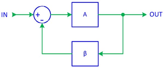
Figure 1.
System with negative feedback.
A well-known property of feedback systems is that when A becomes very large, the equation simplifies to
This principle forms the foundation of active inverse filtering (AIF). It indicates that if the feedback gain is set to β = T(s), then the resulting closed-loop gain is ACL = T−1(s), thereby achieving the desired inverse transfer function. To ensure that this simplification is valid, the forward gain A must be sufficiently large. As a result, AIF operates as a closed-loop system, with the forward gain block consisting of either an integrator or a constant gain unit, while the feedback gain follows the transfer function T(s) of the filter being compensated.
2.2. Gain Elements in Inverse Filtering
Our series of studies on different ADF designs has shown that integrators, when used in closed-loop configurations, can effectively perform various filtering operations [66,67,68,69]. In inverse ADFs, integrators remain the preferred choice for gain elements due to several key advantages. First, unlike conventional gain elements that rely on direct multiplication, integrators operate as summation devices, acting as accumulators rather than simple amplifiers. Second, integrators exhibit extremely high DC gain, with precision being limited only by computational constraints. Third, they are not prone to saturation issues—well-designed digital integrators prevent overflow by ensuring that incremental changes occur at the least significant bits, while the overall bit width maintains accuracy without disrupting signal processing. Finally, in a closed-loop system, an integrator’s forward gain at a given frequency behaves as if squared. For instance, with a sampling interval of T = 0.5 ms, the unity-gain frequency of the integrator is fu = 1/(2πT) = 318 Hz [66]. At 10 Hz, the integrator gain is approximately A = fu/10 ≈ 32, but within a closed-loop configuration, it behaves as an amplifier with an effective gain of A = 322 ≈ 1000, yielding a negligible error of just 1/A = 0.1%. This can be further examined through two specific cases.
Consider Equation (4) in the case of a simple signal follower configuration, where β = 1. Ideally, the closed-loop gain should be ACL = 1, the real gain is (4), and subtracting the ideal gain ACL = 1 and dividing by it results in the gain error:
Now, let us analyze the scenario where the forward gain block A in Figure 1 is an integrator, again assuming β = 1. The digital integrator introduces an approximately 90° phase lag, causing A to be a complex value. As a result, the input–output relationship becomes
Rearranging for ACL = VOUT/VIN, we obtain
Applying a first-order binomial expansion for small x,
The equation simplifies to
Subtracting ACL = 1 and dividing by it yields the gain error:
Comparing the two error expressions for εa and εi, it becomes evident that the error associated with an integrator-based system is equivalent to that of an amplifier with an effective gain of 2A2. For instance, with T = 0.5 ms and fc = 0.05 Hz, the integrator gain is calculated as A = 318/0.05 = 6360, which corresponds to an equivalent amplifier gain of 2 × 63602 = 80,899,200 (approximately 81 million), resulting in an error of merely 0.012 parts per million (ppm).
This analysis highlights why integrators are particularly well-suited as gain elements and error amplifiers in ADFs and especially in AIFs. Their ability to achieve extremely high effective gain with minimal error makes them indispensable for high-precision signal processing applications. However, stability remains a primary concern, and when it must be maintained, the error amplifiers cannot be integrators. Instead, they must be constant-gain amplifiers—gain elements with zero phase delay. While such ideal amplifiers, which provide high constant gain without introducing phase shifts, do not exist in analog signal processing, they can be easily implemented in active DSP filtering.
2.3. Inverse HPF in ECG Processing
This section presents the methodological design of an active inverse high-pass filter (IHPF) aimed at correcting ECG signal distortions introduced by either first- or second-order analog RC high-pass filter (RCHPF). The analog RCHPF is mandatory component in the signal acquisition stage of ECG devices, ensuring the removal of DC offset and low-frequency baseline drift caused by breathing or movements. By incorporating the analog RCHPF, the dynamic range of the amplifiers and ADC can be optimized to scale the ECG amplitude in an enhanced resolution, preventing distortions from signal clipping in the presence of strong low-frequency noise or DC offset. However, the RCHPF introduces distortions in the analog ECG signal, which is then digitized for diagnostic visualization or automated analysis. Therefore, the cutoff frequency of the HPF must be set to the lowest possible level that meets the standards for the intended diagnostic ECG analysis. This method allows for enhanced filtering performance while removing the limitations imposed by the analog RCHPF.
2.3.1. First-Order Inverse HPF
Implementing a first-order active IHPF is straightforward as a digital filter following the analog RCHPF. Based on the scheme in Figure 1, we replace the forward gain A with an integrator and the feedback gain β with an ADF equivalent to the analog RCHPF. The schematic of the resulting inverse filter is shown in Figure 2a. Importantly, the filter is well-suited for real-time processing since it introduces only a minimal delay of one sampling interval.
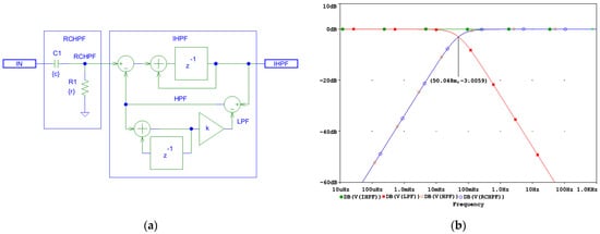
Figure 2.
Design of a digital first-order inverse high-pass filter (IHPF) which corrects the distortions induced by an analog first-order RC high-pass filter (RCHPF): (a) Schematic diagram; (b) frequency response using simulation parameters r and c, which define the time constant τ = rc and the cutoff frequency fc = 1/(2πτ) of the analog RCHPF. The filter is configured for the diagnostic ECG high-pass frequency at fc = 0.05 Hz, with c = 1 µF and r = 1/(2πcfc) = 3.183 MΩ (see the highlighted point at y-axis of −3 dB). IN: input signal; observation nodes: IHPF output (green trace), RCHPF output (blue trace), LPF active low-pass filter in the feedback (red trace), and HPF active high-pass filter in the feedback (orange trace). Note the IHPF output, showing that the first-order high-pass roll-off at the node RCHPF is converted to a flat 0 dB characteristic.
Using an integrator with delay as the forward gain A improves the frequency response of the AIF, ensuring a flat characteristic. The coefficient k in Figure 2a is defined by Equation (12), [66,67,68,69]:
where T is the sampling interval, τ = rc is the time constant, and fc is the high-pass cutoff frequency of the analog RCHPF.
To demonstrate the correct design of the circuit in Figure 2a, it was simulated in the PSpice environment (v. 16.0, Cadence Design Systems Inc., San Jose, CA, USA). The frequency response at different nodes is shown in Figure 2b, while the high-pass cutoff frequency is configured for the diagnostic ECG bandwidth at fc = 0.05 Hz and T = 0.5 ms, yielding the value of k = 0.000157. Figure 2b shows that both the analog RCHPF and digital HPF responses align, with the output IHPF exhibiting a flat 0 dB characteristic. Since the HPF operates within a closed-loop system, stability is maintained, ensuring zero phase shift at high frequencies. However, the DC feedback path remains open. It is important to note that the analog HPF transfer function T(s) features a zero at DC and a real pole at fc. Conversely, its inverse function T−1(s) exhibits a pole at DC and a zero at fc. Consequently, the DC gain theoretically approaches infinity. This means that even a small DC offset Vio at the RCHPF node in Figure 2a would accumulate over time, as illustrated in Figure 3.
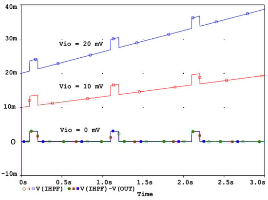
Figure 3.
IHPF behavior with a DC offset Vio = 0, 10 mV, 20 mV. The DC offset Vio is integrated over time and can be corrected by the linear relationship (13).
The behavior of the IHPF circuit from Figure 2a in the presence of a DC offset Vio at the RCHPF node can be analyzed as follows. Consider the integrator as an ideal operational amplifier and the feedback ADF as a high-pass RC network. If the capacitor C initially holds no charge, the circuit reacts by causing the output to jump to Vio, effectively counteracting the offset. Once this offset is established across resistor R, it generates a steady current that gradually charges capacitor C. Given that the time constant of the analog HPF is defined as τ, the output voltage VOUT is
This equation indicates that the output starts at Vio and increases linearly, reaching 2Vio at time t = τ. In real-world applications, the typical offset might reach 10 mV, which can be easily detected and corrected using a software routine. Since Equation (13) describes a linear relationship, implementing this compensation is straightforward, as illustrated in Figure 3.
Figure 3 shows that the DC offset is progressively integrated over time. As explained in the beginning of Section 2.2, in a well-designed active DSP system the digital integrators are inherently resistant to saturation issues because signal changes typically occur in the least significant bits, while saturation in the most significant bits does not compromise signal integrity. Offset compensation can be applied easily without risk of overflow and it can even be adaptively adjusted to correct any residual uncompensated offset, ensuring the long-term accuracy and stability of the reconstructed signal.
2.3.2. Second-Order Inverse HPF
Although second-order high-pass filters are not the standard for ECG diagnostics, they are commonly used in ECG monitoring devices operating in noisy environments, where faster settling times and stronger drift rejection are required. Such devices usually measure the heart rate and various arrhythmia events but are not strictly focused on diagnostic ECG waves, which are distorted. The analog second-order filters are commonly implemented through cascaded first-order RC networks, which provide AC coupling between amplifier stages [23].
Figure 4a shows that the filtering effects of a second-order analog RCHPF can be reversed by cascading two digital first-order IHPFs with the configuration shown in Figure 2a. The total group delay of the two-stage IHPF is two sampling intervals—one from each first-order stage. To validate the circuit design in Figure 4a, the frequency response at different nodes is shown in Figure 4b for a simulation where the high-pass cutoff frequency of each analog RCHPF is set to fc = 0.05 Hz, similarly to the RC network in Figure 2b. Figure 4b illustrates that the second-order roll-off at 0.077 Hz at the RCHPF2 node (blue trace) is transformed into a first-order roll-off at 0.05 Hz at the IHPF1 node (red trace, overlapping with the yellow trace at the RCHPF1 node). This is then corrected to a flat 0 dB response at the output of IHPF2 (green trace). Thus, the restored characteristic completely eliminates the effect of the analog second-order high-pass filtering.
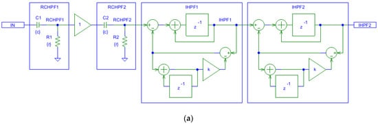
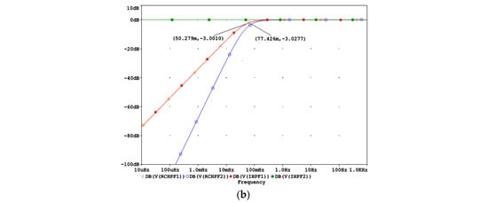
Figure 4.
Design of a digital second-order inverse high-pass filter, cascading two digital first-order inverse high-pass filters (IHPF1 and IHPF2) which correct the distortions induced by an analog second-order RC high-pass filter with two cascaded RC networks (RCHPF1 and RCHPF2): (a) Schematic diagram; (b) frequency response using equal settings for RCHPF1 and RCHPF2 with simulation parameters r and c, providing the cutoff frequency fc = 0.05 Hz for one RC network (c = 1 µF and r = 1/(2πcfc) = 3.183 MΩ). IN: input signal; observation nodes: RCHPF1 output (orange trace), RCHPF2 output (blue trace), IHPF1 output (red trace), and IHPF2 output (green trace). Note that the second-order high-pass roll-off at the RCHPF2 node is converted to a first-order roll-off at the IHPF1 node and then to a flat 0 dB response at the IHPF2 output.
Figure 4 illustrates the implementation of two cascaded first-order IHPFs using separate stages. However, equivalent functionality can be achieved more efficiently by using a single integrator in the forward path and cascading two first-order HPFs in the feedback. This configuration is more economical because it eliminates the need for a second IHPF stage. It is important to note that in IHPF implementations, the feedback transfer function can be of second-or-higher-order without suffering from the stability problems. Therefore, if the analog front-end uses a second-or-higher-order HPF, such as Bessel, Butterworth, or Chebyshev, the feedback HPF must be designed to accurately replicate its characteristics for efficient signal recovery.
2.4. Inverse LPF in ECG Processing
This section presents the methodological design of an active inverse low-pass filter (ILPF) aimed at correcting ECG signal distortions introduced by either a first- or second-order analog RC low-pass filter (RCLPF). Diagnostic ECG signals are first-order low-pass filtered with a cutoff frequency of 150 Hz to preserve the high-frequency diagnostic components usually associated with sharp transitions in QRS complexes and late potentials. However, such cutoffs are impractical for continuous monitoring in noisy environments with significant motion artifacts, high-frequency EMG noise, and various interferences. Therefore, for ECG monitoring, the LPF cutoff is typically reduced to 40 Hz [18,19], and for ventricular arrhythmia detection in automated external defibrillators, it is lowered further to 30 Hz [20] in a trade-off between ECG distortions and robustness against noise that can compromise the automated rhythm analysis. The proposed further ILPF concept is directed towards restoring ECG diagnostic features while allowing the use of stronger analog RCLPF for improved noise immunity.
2.4.1. First-Order Inverse LPF
In the active ILPF design, the feedback gain in Figure 1 should correspond to the ADF equivalent of the analog LPF. However, unlike in IHPFs, the forward gain cannot be an integrator. Using an integrator would render the system unstable, as the LPF transfer functions introduce a second dominant pole in the loop. Instead, the forward gain should be a constant-gain unit with no phase shift, ensuring stability and accurate closed-loop inverse filtering. This type of forward gain block is not readily available in analog processing because real-world analog amplifiers, including operational amplifiers and transistor stages, inherently behave as integrators or lossy integrators. Advantageously, digital signal processing enables the implementation of a true constant gain block, making ILPFs feasible and effective.
The schematic and the frequency response of the designed first-order ILPF are shown in Figure 5. In this implementation, the forward gain A is set to A = 10,000, ensuring an accuracy of 1/A = 0.01% and providing a dynamic range of 80 dB, sufficient for ECG signal restoration. This high forward gain allows the ILPF to effectively correct signal distortions introduced by the conventional real-pole LPF while preserving stability. The frequency response in Figure 5b illustrates a bandwidth extension from 30 Hz at the RCLPF node to approximately 882 Hz at the ILPF output, approaching the Nyquist frequency of 1 kHz for a system operating with a sampling interval of T = 0.5 ms.
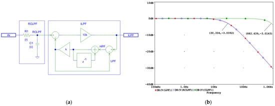
Figure 5.
Design of a digital first-order inverse low-pass filter (LHPF) which corrects the distortions induced by an analog first-order RC low-pass filter (RCLPF): (a) Schematic diagram; (b) frequency response using simulation parameters r and c, which define the time constant τ = rc and the cutoff frequency fc = 1/(2πτ) of the analog RCLPF. The filter is configured for fc = 30 Hz, with c = 1 µF and r = 1/(2πcfc) = 5.3 kΩ (see the highlighted point at y-axis of −3 dB). IN: input signal; observation nodes: ILPF output (green trace), RCLPF output (blue trace), and LPF active low-pass response in the feedback (red trace), with the red trace overlapping the blue trace. Note that the first-order low-pass response at the RCLPF node is converted to a flat 0 dB response up to 882 Hz, limited by the Nyquist frequency (1 kHz).
As shown in Figure 5a, the first-order ILPF does not introduce a delay and compensates for the group delay of the RCLPF; thus, it is well-suited for real-time processing.
2.4.2. Second-Order Inverse LPF
The design of the second-order ILPF schematic is shown in Figure 6a. It uses a cascade of two first-order digital ILPFs (ILPF1 and ILPF2) which compensate for higher-order cascaded filtering stages with real poles, such as the two first-order analog RCLPFs (RCLPF1 and RCLPF2). However, to ensure system stability, it is crucial that the ILPF feedback path contains one dominant pole. This dominant pole prevents instability by limiting the overall loop gain at high frequencies to a first-order roll-off, ensuring stable inverse filtering. The ILPF1 and ILPF2 do not introduce delay and compensate the group delay of the RCLPF1 and RCLPF2; thus, the second-order ILPF is well suited for real-time operation.
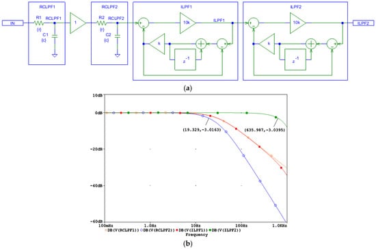
Figure 6.
Design of a digital second-order inverse low-pass filter, cascading two digital first-order inverse low-pass filters (ILPF1 and ILPF2) which correct the distortions induced by an analog second-order RC low-pass filter with two cascaded RC networks (RCLPF1 and RCLPF2): (a) Schematic diagram; (b) frequency response using equal settings for RCLPF1 and RCLPF2 with simulation parameters r and c, providing the cutoff frequency fc = 30 Hz for one RC network (c = 1 µF and r = 1/(2πcfc) = 5.3 kΩ). IN: input signal; observation nodes: RCLPF1 output (orange trace), RCLPF2 output (blue trace), ILPF1 output (red trace), and ILPF2 output (green trace). Note that the second-order low-pass response at the node RCLPF2 is converted to a first-order low-pass roll-off at the node ILPF1, and then to a flat 0 dB response up to 635 Hz limited by the Nyquist frequency (1 kHz).
To validate the circuit design in Figure 6a, the frequency response at different nodes is shown in Figure 6b for a simulation where the low-pass cutoff frequency of each analog RCLPF is set to fc = 30 Hz, similarly to the RC network in Figure 5b. Figure 6b illustrates the bandwidth extension, starting from a second-order low-pass roll-off at approximately 19 Hz at the RCLPF2 node (blue trace), followed by a first-order roll-off at 30 Hz at the ILPF1 node (red trace, overlapping with the magenta trace at the RCLPF1 node), and finally resulting in a flat 0 dB response extending up to approximately 635 Hz at the ILPF2 output (green trace). Due to the inherent limitations of ILPF1 reconstruction at frequencies near the Nyquist frequency (1 kHz), the observed cutoff frequency of 635 Hz is slightly lower than the 882 Hz seen for the first-order ILPF in Figure 5b. This indicates that the reconstruction bandwidth, which eliminates the effect of the analog low-pass filtering, is fundamentally constrained by the Nyquist limit.
Figure 6 illustrates the implementation of two cascaded first-order ILPF stages. To ensure system stability, the feedback path of an ILPF must not contain higher-order low-pass filters. As a result, each ILPF stage can only compensate for a single first-order analog LPF. For compensating higher-order analog LPFs, multiple ILPF stages should be cascaded accordingly.
3. Results
3.1. Test of High-Pass Filters with Impulse Signals
According to the international IEC 60601-2-25:2011 standard [17], which defines the essential performance requirements for electrocardiographs, the low-frequency (impulse) response is evaluated using a test rectangular pulse with an amplitude of 3 mV and a duration of 100 ms. This test must ensure that the baseline displacement after the pulse does not exceed ±100 µV relative to the baseline before the pulse. We further refer to this displacement as the “undershoot magnitude”, which is measured in Figure 7 for both first- and second-order RCHPFs and followed by their corresponding digital IHPFs according to the schemes in Figure 2a and Figure 4a. In Figure 7, it is clearly observed that the undershoot magnitude is larger for second-order vs. first-order RCHPFs, as well as for RCHPFs with a cutoff frequency of 1 Hz vs. 0.05 Hz. Notably, no discernible undershoot is present in any of the IHPFs’ outputs, demonstrating their effective compensation of the analog filter distortions.
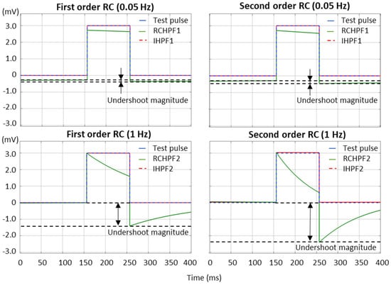
Figure 7.
Performance of first- and second-order RC high-pass filter (RCHPF) and inverse high-pass filter (IHPF) with a test rectangular pulse (3 mV, 100 ms), using an RC cutoff frequency setting of 0.05 Hz (top) and 1 Hz (bottom). RCHPF1, IHPF1: Measurements at the RCHPF and IHPF nodes, respectively, of the first-order scheme in Figure 2a. RCHPF2, IHPF2: Measurements at the RCHPF2 and IHPF2 nodes, respectively, of the second-order scheme in Figure 4a. The baseline displacement, referred to as the ‘undershoot magnitude’, is illustrated.
The undershoot magnitudes are measured over a broad range within the low-frequency bandwidth of ECG signals by configuring the analog RC networks in Figure 2a and Figure 4a with cutoff frequencies ranging from 0.05 to 5 Hz. The results are presented in Figure 8. First- and second-order RCHPFs with cutoff frequencies of 0.5 Hz and above exhibit significant undershoot magnitudes between –1500 µV and –3300 µV, consistent with the example shown in Figure 7 (bottom plot). Among all tested configurations, only the first-order RCHPF set at 0.05 Hz, with an undershoot amplitude of −85 μV, complies with the IEC 60601-2-25 standard [17]. Adding a second stage at 0.05 Hz doubles the undershoot, exceeding the standard’s limits, as illustrated in Figure 7. In contrast, adding the first- and second-order inverse high-pass filters (IHPF1 and IHPF2) after the RCHPF substantially reduced undershoot magnitudes—remaining below 5 μV for cutoff frequencies up to 1 Hz, below 10 μV up to 2 Hz, and not exceeding 25 μV even for higher cutoff frequencies up to 5 Hz. All these values are well within the IEC 60601-2-25:2011 compliance limit.
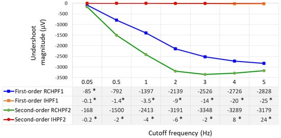
Figure 8.
Undershoot magnitudes measured as a response of first- and second-order RC high-pass filter (RCHPF) and inverse high-pass filter (IHPF) with a test rectangular pulse (3 mV, 100 ms), using a RC cutoff frequency setting from 0.05 Hz to 5 Hz. RCHPF1, IHPF1: Measurements at the RCHPF and IHPF nodes, respectively, of the first-order scheme in Figure 2a. RCHPF2, IHPF2: Measurements at the RCHPF2 and IHPF2 nodes, respectively, of the second-order scheme in Figure 4a. *: Undershoot magnitudes below 100 μV, in compliance with the IEC 60601-2-25:2011 standard [17].
It is worth noting that the IHPF fully complies with the IEC 60601-2-25:2011 standard in relation to the other two performance criteria defined for the test rectangular pulse (3 mV, 100 ms):
- The slope outside the pulse shall be less than 0.3 mV/s, according to the measurements for the 0.05 Hz first-order RC filter. This requirement is satisfied, as evidenced by the fact that the IHPF’s undershoot amplitude is more than three times smaller than that of the 0.05 Hz RC filter.
- The leading edge overshoot shall be less than 10%. All our measurements confirm that both first- and second-order RCHPFs and IHPFs consistently reproduce the leading edge of the rectangular pulse without introducing any overshoot (as illustrated in Figure 7).
3.2. Test of High-Pass Filters with Standard ECG Signals
Validation that high-pass filters preserve the fidelity of the diagnostic ECG waveform is done according to the IEC 60601-2-25:2011 standard [17], using as a reference the artificially generated ECG-like signals with well-defined amplitude–time characteristics from the “Conformance Testing Services For Computerized Electrocardiography”, namely, the CTS-ECG database [70]. We use the eight ECG leads (I, II, and V1–V6) available in the analytical signal ANE20000. The standard requirements focus on the following:
- ST amplitudes taken between 20 and 80 ms after QRS-offset that shall not deviate by more than ±25 μV from the reference amplitude of the standard ECG signals;
- Output peak amplitudes for R- and S-waves that shall not deviate by more than 5% from the original values.
An example of the RCHPF and IHPF performance using two ECG leads—lead I and lead V2, with the largest (steepest) signal—are presented in Figure 9. The positions for the measurements of the R-peak, S-peak, and ST-segment are indicated by dotted vertical lines.
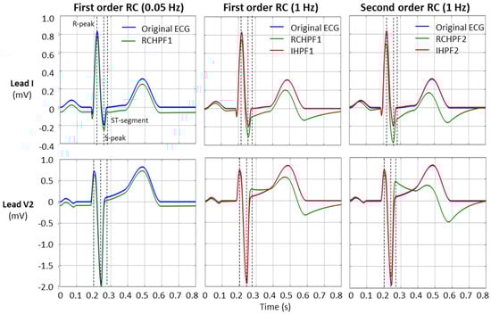
Figure 9.
Performance of first- and second-order RC high-pass filter (RCHPF) and inverse high-pass filter (IHPF) with standard ECG (leads I and V2) from file ANE20000, using RC cutoff frequencies of 0.05 Hz (diagnostic) and 1 Hz. RCHPF1, IHPF1: Measurements at the RCHPF and IHPF nodes, respectively, of the first-order scheme in Figure 2a. RCHPF2, IHPF2: Measurements at the RCHPF2 and IHPF2 nodes, respectively, of the second-order scheme in Figure 4a. Dotted vertical lines: Positions for the measurements of the R-peak, S-peak, and ST-segment on each ECG lead.
The measurements of R-peak, S-peak, and ST-segment are further applied to the eight ECG leads while the RC constants of all filters in Figure 2a and Figure 4a are configured a broad low-frequency ECG range from 0.5 to 5 Hz. Statistical analysis of the results is presented in Figure 10 and Table 1. The following observations can be drawn:
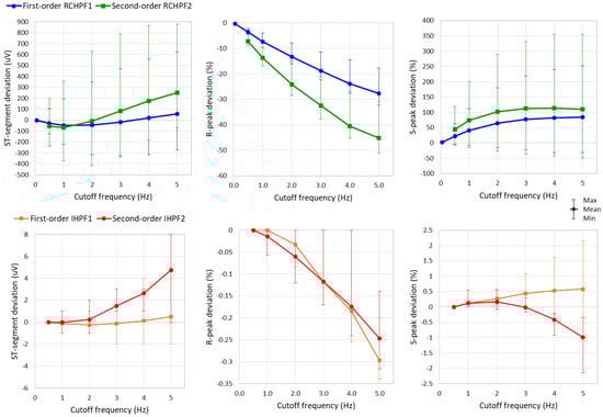
Figure 10.
Graph for the ST-segment deviation, R-peak deviation, and S-peak deviation on a standard ECG (ANE20000) filtered with a first- and second-order RC high-pass filter (RCHPF) and inverse high-pass filter (IHPF) with RC cutoff frequency setting from 0.5 Hz to 5 Hz. Graphs are presented as mean values (dots) and min–max ranges (whiskers) across the 8 ECG leads (I, II, and V1–V6). RCHPF1, IHPF1: Measurements at the RCHPF and IHPF nodes, respectively, of the first-order scheme in Figure 2a. RCHPF2, IHPF2: Measurements at the RCHPF2 and IHPF2 nodes, respectively, of the second-order scheme in Figure 4a.

Table 1.
Numerical data for the ST-segment deviation, R-peak deviation, and S-peak deviation on a standard ECG (ANE20000) filtered with a first- and second-order RC high-pass filter (RCHPF) and inverse high-pass filter (IHPF) with RC cutoff frequency setting from 0.5 Hz to 5 Hz. Data are reported as mean value (min–max range) across the 8 ECG leads (I, II, and V1–V6). RCHPF1, IHPF1: Measurements at the RCHPF and IHPF nodes, respectively, of the first-order scheme in Figure 2a. RCHPF2, IHPF2: Measurements at the RCHPF2 and IHPF2 nodes, respectively, of the second-order scheme in Figure 4a.
- The ST-segment deviation caused by high-pass filters significantly exceeds the ±25 μV limit, even at the monitoring cutoff frequency of 0.5 Hz, reaching up to −125 μV and −240 μV for the first- and second-order RCHPF, respectively. In contrast, the inverse HP filters substantially reduce ST-segment deviation, keeping the maximum deviation of any lead below 5 μV even at cutoff frequencies as high as 5 Hz—ten times higher than the monitoring setting. Thus, the ST-segment deviation with IHPF is comparable to that of a diagnostic first-order RCHPF (0.05 Hz), which we measured for the standard signal ANE20000 (leads I, II, and V1–V6) to have a mean value of −2.8 μV, with a minimum–maximum range of (−13 μV to +12 μV).
- The effect of high-pass filters on other ECG waves includes a reduction in the amplitude of the positive R-peak, showing negative deviations ranging from −3.6% to −28% (mean values) and up to −4.5% to −32% (maximum deviations). Additionally, high-pass filters overdamp the negative S-peak, causing positive deviations from 7% to 45% (mean values) and up to 119% to 355% (maximum deviations). In contrast, the inverse high-pass filters substantially reduce R-peak deviations to below −3.5% and S-peak deviations to below ±2%, even at the highest cutoff frequency of 5 Hz. These results remain well within the recommended deviation limit of ±5% [17].
3.3. Test of Low-Pass Filters with Impulse Signals
The high frequency filter response can be measured with different test signals. In Figure 11, we present the test signals used in this study, as follows:
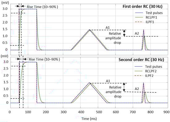
Figure 11.
Performance of first- and second-order RC low-pass filter (RCLPF) and inverse low-pass filter (ILPF) with calibration pulses, including a rectangular pulse (3 mV, 100 ms), triangular pulse (1.5 mV, 200 ms), and triangular pulse (1.5 mV, 20 ms), using the RC cutoff frequency setting of 30 Hz. RCLPF1, ILPF1: Measurements at the RCLPF and ILPF nodes, respectively, of the first-order scheme in Figure 5a. RCLPF2, ILPF2: Measurements at the RCLPF2 and ILPF2 nodes, respectively, of the second-order scheme in Figure 6a. The fiducial points used to measure the rise time (10–90%) and relative amplitude drop are illustrated.
- Square test impulse: The rise time, defined as the time required for the filtered signal to transition from 10% to 90% of the rising edge, is a common metric in signal processing used to assess filter performance. Although no specific limits are established for this metric in ECG signal processing, we report it here for completeness and comparative analysis. The same square test impulse (3 mV, 100 ms) used for the high-pass filter evaluation in Section 3.1 is applied.
- Triangular test pulses with varying width are used for ECG processing test sets because they simulate R-waves with different steepness. The IEC 60601-2-25:2011 standard for diagnostic electrocardiographs [17] allows from 0 down to −10% reduction in the peak amplitude of a triangular pulse (1.5 mV, 20 ms) compared to a triangular pulse (1.5 mV, 200 ms). This metric is further named the relative amplitude drop, measured using the amplitudes A1 and A2 in Figure 11:
Relative amplitude drop and rise time (10–90%), using the test signals shown in Figure 11, are measured across a broad range within the high-frequency bandwidth of ECG signals by configuring the analog RC networks in Figure 5a and Figure 6a with cutoff frequencies ranging from 10 Hz to 150 Hz—the maximum diagnostically relevant frequency specified by the standard [17]. The results are presented in Figure 12. RCLPFs with cutoff frequencies up to 100 Hz (first-order) and up to 150 Hz (second-order) exhibit significant amplitude drop between –70% and –10%, consistent with the examples shown in Figure 11. Among all tested configurations, only the first-order RCLPF set at 100 to 150 Hz, with an undershoot amplitude of −9.9% down to −6.4%, complies with the −10% limit of the IEC 60601-2-25 standard [17]. In contrast, adding inverse high-pass filters after the RCLPF substantially reduced undershoot magnitudes—keeping them below 0.2% for the first-order ILPF1 and below 2.5% for the second-order ILPF2.
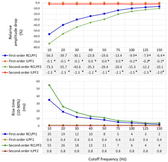
Figure 12.
Relative amplitude drop of a triangular pulse ((1.5 mV, 20 ms vs. 200 ms) (on top), and rise time (10–90%) of a rectangular impulse (on bottom) produced by a first- and second-order RC low-pass filter (RCLPF) and inverse low-pass filter (ILPF), using an RC cutoff frequency setting from 10 Hz to 150 Hz. RCLPF1, ILPF1: Measurements at the RCLPF and ILPF nodes, respectively, of the first-order scheme in Figure 5a. RCLPF2, ILPF2: Measurements at the RCLPF2 and ILPF2 nodes, respectively, of the second-order scheme in Figure 6a. *: Relative amplitude drop not exceeding −10%, in compliance with the IEC 60601-2-25:2011 standard [17].
Rise times (10–90%) are substantial for RCLPFs with cutoff frequencies below 50 Hz, ranging from 8 to 35 ms for first-order and from 11 to 55 ms for second-order filters, while they decrease to 2 ms and 4 ms, respectively, when the cutoff frequency is increased to 150 Hz. Usefully, inverse low-pass filters exhibit stable and significantly shorter rise times—0.4 ms for first-order and 0.8 ms for second-order—regardless of the cutoff frequency.
3.4. Test of Low-Pass Filters with Standard ECG Signals
Validation of low-pass filters for preserving the fidelity of the diagnostic ECG waveform, in accordance with the IEC 60601-2-25:2011 standard [17], was performed using the same standard ECG file (ANE20000) as used for the high-pass filter validation in Section 3.2. Since low-pass filters primarily affect high-frequency components of the ECG, the standard specifies that reductions in the amplitudes of the R- and S-peaks must not exceed 5% of their original values. Figure 13 illustrates the effect of low-pass filtering and its inverse application on the ECG signal (leads I and V2). To better demonstrate the reduction in R- and S-wave amplitudes, the filters are configured with a low cutoff frequency of 30 Hz. The fiducial points for measuring the R- and S-peaks are indicated by dotted vertical lines.
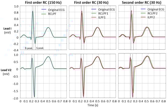
Figure 13.
Performance of first- and second-order RC low-pass filter (RCLPF) and inverse low-pass filter (ILPF) with standard ECG (leads I and V2) from file ANE20000, using an RC cutoff frequency setting of 150 Hz (diagnostic) and 30 Hz. RCLPF1, ILPF1: Measurements at the RCLPF and ILPF nodes, respectively, of the first-order scheme in Figure 5a. RCLPF2, ILPF2: Measurements at the RCLPF2 and ILPF2 nodes, respectively, of the second-order scheme in Figure 6a. Dotted vertical lines: Positions for the measurements of the R-peak and S-peak on each ECG lead.
Measurements of R- and S-peaks were further extended to all eight ECG leads, with the RC constants of all filters shown in Figure 5a and Figure 6a configured across a broad high-frequency ECG range from 10 to 150 Hz. A statistical analysis of the results is presented in Figure 14 and Table 2. The maximum reduction of the positive R-peak amplitude remains below 5% in all ECG leads when using first-order RCLPF1 filters (≥50 Hz) and second-order RCLPF2 (≥75 Hz). The reduction of the negative S-peak amplitude is approximately 2.5 times larger than that of the R-peak, limited below 5% for RCLPF1 (≥75 Hz) and RCLPF2 (≥125 Hz). Figure 14 (top plots) shows that low-pass filters with cutoff frequencies as low as 10 Hz can reduce R-peak amplitudes by up to 60% and S-peak amplitudes by up to 130%. In contrast, inverse low-pass filters significantly reduce these distortions, keeping R-peak deviations below −0.3% and S-peak deviations below −1%, even at the lowest cutoff frequency of 10 Hz.
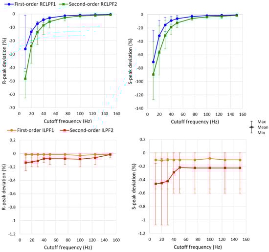
Figure 14.
Graph for the R-peak and S-peak deviations on a standard ECG (ANE20000) filtered with a first- and second-order RC low-pass filter (RCLPF) and inverse low-pass filter (ILPF) setup at an RC cutoff frequency from 10 Hz to 150 Hz. Graphs are presented as mean values (dots), min–max ranges (whiskers) across the 8 ECG leads (I, II, and V1–V6). RCLPF1, ILPF1: Measurements at the RCLPF and ILPF nodes, respectively, of the first-order scheme in Figure 5a. RCLPF2, ILPF2: Measurements at the RCLPF2 and ILPF2 nodes, respectively, of the second-order scheme in Figure 6a.
Table 2.
Numerical data for the R-peak and S-peak deviations on a standard ECG (ANE20000) filtered with a first- and second-order RC low-pass filter (RCLPF) and inverse low-pass filter (ILPF) setup at an RC cutoff frequency from 10 Hz to 150 Hz. Data are reported as mean value (min–max range) across the 8 ECG leads (I, II, and V1–V6). RCLPF1, ILPF1: Measurements at the RCLPF and ILPF nodes, respectively, of the first-order scheme in Figure 5a. RCLPF2, ILPF2: Measurements at the RCLPF2 and ILPF2 nodes, respectively, of the second-order scheme in Figure 6a.
4. Discussion
In this paper, we have introduced novel active inverse filtering techniques which are capable of accurately restoring ECG signals distorted by high-pass and low-pass analog RC filters. Traditional analog filters cause distortions in diagnostic ECG components like the QRS morphology and the ST-segment level, which may lead to incorrect diagnosis. Using inverse filtering, these distortions can be corrected, helping to restore the true ECG signal waveform and improving the accuracy of interpretation for reliable diagnosis of cardiac conditions such as myocardial infarction, ischemia, arrhythmias, conduction disturbances, electrolyte imbalances, and other disorders that require precise assessment of ECG wave amplitudes and durations.
Diagnostic ECG devices use an analog HPF with a cutoff frequency of 0.05 Hz. However, this setting is very strict and leaves no room for adding extra high-pass filtering later in the digital processing stage. If either the cutoff frequency or the order of the analog filter is increased, the resulting distortions exceed acceptable limits. For example, even for the low 0.5 Hz cutoff, the undershoot magnitude of RCHPF1 is 790 µV and RCHPF2 is 1500 µV (Figure 8), which is much higher than the limit of 100 µV; the ST-segment deviation reaches up to −125 μV (RCHPF1) and −240 μV (RCHPF2), above the ±25 μV limit; the maximal deviation of the R-peak is −4.5% (RCHPF1) and −8.8% (RCHPF2) and that of the S-peak is 62% (RCHPF1) and 120% (RCHPF2), above the limit of 5% (Table 1, Figure 10). The proposed IHPFs resolve this issue by restoring the ECG signal to its original waveform before the analog HPF application. This is illustrated in Figure 9 and validated using standard ECG signals (Figure 10, Table 1) and transient analysis with a rectangular test signal (Figure 7 and Figure 8). Both first- and second-order IHPFs, operating over a broad low-frequency range (0.05–5 Hz), comply with the IEC 60601-2-25:2011 standard in respect to ST-segment deviations <5 μV (within ±25 μV limit) and R- and S-peak deviations <±3.5% (within ±5% limit), with undershoot magnitudes of 0.1–25 µV (within ±100 µV limit) and no overshoot or excessive slopes as after effects <0.3 mV/s. These results confirm that IHPFs can enable effective high-pass refiltering in DSP.
However, the restored signals are not immediately suitable for direct interpretation and require additional digital HPF processing. One limitation of IHPFs is their sensitivity to DC offset and the choice of the cutoff frequency in the analog HPF. The DC offset is integrated by the IHPF, causing a signal drift over time. The example in Figure 3 demonstrates that with a DC offset of 10 mV and a filter time constant of 3.18 s (corresponding to a cutoff frequency of 0.05 Hz), the offset increases by an additional 10 mV after 3.18 s. If the cutoff frequency is increased to 5 Hz, the same offset accumulates within just 31.8 ms, and after 3.18 s, it reaches 1000 mV. Thus, as the cutoff frequency increases, the drift accelerates, making offset compensation more challenging. To address this, special procedures must be implemented to estimate and subtract the offset before applying the IHPF. Developing real-time DC offset compensation is particularly important for capacitive electrode-based ECG sensing, where achieving a lower cutoff frequency is difficult, and the analog front-end typically operates with a few-hertz high-pass cutoff [71]. The presented inverse filter implementation is capable of working in such capacitive coupling scenarios using either a first-order stage or a second-order stage by cascading two first-order IHPFs. Active inverse filtering is a straightforward approach and implementing IHPF in capacitive electrode front-ends can significantly enhance ECG signal quality by effectively compensating for signal distortions and restoring critical waveform details.
Accurate signal reconstruction requires the digital equivalent of the analog RC filter in the feedback path to closely match the characteristics of the actual analog filter. However, analog components inherently exhibit manufacturing tolerances, typically around 1% for resistors and up to 10% for capacitors, resulting in potential cutoff frequency deviations of up to 11%. These deviations can be effectively compensated by adjusting the coefficient k and fine-tuning the cutoff frequency of the digital feedback filter. To ensure proper alignment, prior calibration of the feedback path is essential. This calibration process can be implemented as a self-calibrating routine, enabling automatic compensation for component variations.
It is worth noting that our active IHPF approach is fundamentally different from existing methods such as those presented in Abächerli et al. [61] and Kowada et al. [62,63]. In contrast to published techniques, our design approach uniquely integrates the digital equivalent of the analog filter into the feedback path of a closed-loop system. This makes the active IHPF a creative and original solution for restoring ECG signals. The proposed filter enables ECG signals to be acquired using AC-coupled analog front-ends [72,73,74] with high cutoff frequencies that enable faster analog settling. This study validates that, with the use of the IHPF, cutoff frequencies can be increased from the typical monitoring range of 0.5–1 Hz to as high as 5 Hz, while ECG distortions still remain well within the standard limits. Furthermore, the IHPF can be applied to ECG samples digitized by SAR ADCs in real-time because the filter design introduces a delay of just one sampling interval per stage (Figure 2a and Figure 4a). After reconstruction by the IHPF, ECG signals can be further processed with any application-specific digital HPF, meaning that DSP algorithms are no longer constrained by the limitations of the acquisition stage. This also helps avoid inconsistencies in digital ECG databases used for machine learning.
Generally, analog RC low-pass filters fail to comply with the IEC 60601-2-25:2011 standard for cutoff frequencies below 150 Hz. Our calibration tests show a significant triangular pulse amplitude drop (10–70%) for cutoff frequencies up to 100 Hz (RCLPF1) and up to 150 Hz (RCLPF2) (Figure 12); large R-peak amplitude reduction (5–60%) for cutoff frequencies ≤50 Hz (RCLPF1) and ≤75 Hz (RCLPF2) (Table 2) and a 2.5 times larger S-peak amplitude reduction, limited below 5% for RCLPF1 (≥75 Hz) and RCLPF2 (≥125 Hz).
Unlike IHPFs, inverse low-pass filter designs cannot use an integrator-based forward gain, as it would cause system instability. Instead, a high-gain constant amplifier is used, ensuring no phase shift and accurate signal reconstruction. A second-order ILPF, implemented by cascading two first-order ILPFs, further enhances the restoration precision for ECG signals subjected to second-order low-pass filtering. This is illustrated in Figure 13 and validated using standard ECG signals (Figure 14, Table 1) and transient analysis with rectangular and triangular test signals (Figure 11 and Figure 12). Both first- and second-order ILPFs, operating over a broad high-frequency range (10–150 Hz), comply with the IEC 60601-2-25:2011 standard in respect to R- and S-peak suppression of less than −1% (within ±5% limit) and a relative amplitude drop of only 0.2–2.5%, far below the 10% limit for peak amplitude reduction of a triangular pulse (1.5 mV) with 20 ms vs. 200 ms widths. The ILPFs demonstrate stable performance with rise times up to 80 times shorter than RCLPFs—0.4 ms for the first-order and 0.8 ms for the second-order—regardless of the cutoff frequency, which can be as low as 10 Hz. These results confirm that ILPFs can enable the effective low-pass refiltering in DSP. It is important to note that although the restored bandwidth at the IHPF output approaches the Nyquist frequency (Figure 5b and Figure 6b), the increased bandwidth also amplifies noise along with the ECG signal. Therefore, the signal bandwidth should always be limited to the minimum necessary to preserve diagnostically relevant ECG information for the specific application. If the sampling rate is too low, the signal should be upsampled before applying the ILPF and then downsampled after processing. Additionally, ADC quantization noise is emphasized, therefore requiring low-pass or median filtering to limit bandwidth and minimize noise that can disturb diagnostic precision.
The proposed inverse filtering techniques provide an effective digital solution for recovering ECG signals distorted by traditional analog filtering. First-order IHPF and ILPF implementations are sufficient for most ECG applications, while second-order versions are required to compensate for higher-order analog filters. Combining active inverse filtering with digital compensation techniques improves ECG signal quality and thus diagnostic reliability in automated ECG analysis. Future work may focus on developing distortion-free HPFs to effectively suppress baseline wander while preserving the original shape, amplitude, phase, and timing of key ECG features in the reconstructed signals. Further optimization of signals reconstructed by ILPFs for specific applications warrants investigation. This could involve implementing linear-phase LPFs to preserve waveform fidelity or adaptive LPFs that adjust dynamically to signal characteristics, ensuring robust performance under varying conditions [32,36,42,50,51].
Before the development of the ADF approach, active inverse filtering was unknown in DSP applications. This paper can serve as a tutorial on how active inverse systems can be successfully implemented in closed-loop configurations. This work establishes that both IHPFs and ILPFs are not only theoretically feasible in active DSP but also offer simple and practical solutions for real-world applications. Moreover, the potential of active inverse filtering extends beyond biomedical signals, with promising applications in areas such as audio, video, and image processing—opening new opportunities for advanced signal restoration techniques.
5. Limitations of This Study
This version of the inverse high-pass filter does not deal with DC offsets. Since the IHPF uses an integrator in the forward path, any DC component is progressively accumulated over time, leading to drift and potential saturation in long-term operation. To address this limitation, the DC offset must be accurately estimated and subtracted before applying the IHPF. Adaptive offset cancellation techniques or pre-filtering routines can be employed to suppress or remove the DC component, ensuring that the IHPF reconstructs the signal without a drift.
Another limitation is that the feedback path of the inverse filter’s closed-loop system must digitally replicate the analog RC filter. However, component tolerances could lead to the deviation of the cutoff frequency from its nominal value. Therefore, to maintain alignment between the analog and digital inverse filters, prior calibration of the feedback path is essential.
6. Conclusions
The design of active inverse filters is intuitive and follows a straightforward procedure. It involves a closed-loop configuration where the forward path consists of a gain element, either an integrator or a constant-gain amplifier, while the feedback path incorporates the digital equivalent of the analog filter being compensated. This implementation is conceptually clear and does not require complex mathematical derivations to understand the underlying operational principles. The simplicity of the structure makes it accessible and practical for real-world applications.
The paper also can serve as a tutorial, offering clear explanations of closed-loop inverse filtering from theoretical design to practical implementation. Validated with standard-compliant ECG test signals, this method proves to be reliable and shows strong potential for use in various biomedical applications. It can operate on popular microcontrollers with a minimal signal delay of one or two sampling intervals, making it well-suited for wearable devices and continuous monitoring systems.
Future developments may focus on enhancing the system’s robustness and clinical usability, including advanced automated procedures for DC offset estimation and removal prior to the application of IHPFs, especially in systems with capacitive electrodes, or new IHPF designs which compensate the DC offset itself. The design of minimal-distortion filters for the restored ECG signals after inverse filtering is also a valuable direction for further research.
Author Contributions
Conceptualization, D.D. and T.N.; methodology, D.D. and T.N.; software, D.D. and T.N.; validation, D.D., T.N., V.K. and I.J.; formal analysis, D.D., T.N., V.K. and I.J.; investigation, D.D., V.K. and I.J.; resources, D.D. and T.N.; data curation, D.D. and T.N.; writing—D.D., T.N., V.K. and I.J.; writing—review and editing, D.D., T.N., V.K. and I.J.; visualization, D.D., T.N. and V.K.; supervision, V.K. and I.J.; project administration, D.D.; funding acquisition, V.K. and I.J. All authors have read and agreed to the published version of the manuscript.
Funding
This research was funded by the Bulgarian National Science Fund, grant number KП-06-H42/3.
Institutional Review Board Statement
Not applicable.
Data Availability Statement
Data are contained within the article.
Conflicts of Interest
The authors declare no conflicts of interest.
Abbreviations
The following abbreviations are used in this manuscript:
| ECG | electrocardiogram |
| RC | resistor–capacitor network |
| ADC | analog-to-digital converter |
| SAR | successive approximation register |
| LPF | low-pass filter |
| HPF | high-pass filter |
| DSP | digital signal processing |
| ADF | active digital filter |
| AIF | active inverse filter |
| IHPF | inverse high-pass filter |
| ILPF | inverse low-pass filter |
| RCHPF | RC high-pass filter |
| RCLPF | RC low-pass filter |
| DC | direct current |
| AC | alternating current |
| BWL | baseline wander |
| EMG | electromyogram |
References
- Brady, W.J.; Lipinski, M.J.; Darby, A.E.; Bond, M.C.; Charlton, N.P.; Hudson, K.B.; Williamson, K. Electrocardiogram in Clinical Medicine, 1st ed.; John Wiley & Sons Ltd.: Hoboken, NJ, USA, 2020; pp. 1–512. [Google Scholar]
- Dotsinsky, I.; Christov, I.; Levkov, C.; Daskalov, I. A microprocessor–electrocardiograph. Med. Biol. Eng. Comput. 1985, 23, 209–212. [Google Scholar] [CrossRef] [PubMed]
- Filomena, E.; Aldonate, J. Portable wireless device for biopotential recording. In Proceedings of the 2013 Fourth Argentine Symposium and Conference on Embedded Systems (SASE/CASE), Buenos Aires, Argentina, 14–16 August 2013. [Google Scholar] [CrossRef]
- Analog Devices. ECG Front-End Design Is Simplified with MicroConverter. Analog Dialogue. 2003, pp. 37–11. Available online: https://www.analog.com/en/resources/analog-dialogue/articles/ecg-front-end-design-simplified.html (accessed on 9 March 2025).
- Strauss, D.; Schocken, D. Marriott’s Practical Electrocardiography, 13th ed.; Lippincott Williams & Wilkins (LWW): Philadelphia, PA, USA, 2021. [Google Scholar]
- Daskalov, I.; Dotsinsky, I.; Christov, I. Developments in ECG acquisition, preprocessing, parameter measurement and recording. IEEE Eng. Med. Biol. Mag. 1998, 17, 50–58. [Google Scholar] [CrossRef] [PubMed]
- Sörnmo, L.; Laguna, P. Chapter 6—The Electrocardiogram—A Brief Background. In Biomedical Engineering, Bioelectrical Signal Processing in Cardiac and Neurological Applications; Sörnmo, L., Laguna, P., Eds.; Academic Press: Cambridge, MA, USA, 2005; pp. 411–452. [Google Scholar] [CrossRef]
- Merletti, R.; Ceronee, G. Tutorial. Surface EMG detection, conditioning and pre-processing: Best practices. J. Electromyogr. Kinesiol. 2020, 54, 102440. [Google Scholar] [CrossRef] [PubMed]
- Ganev, B.; Iliev, I.; Jekova, I.; Krasteva, V. LabVIEW ECG and Noise Simulator for Advanced Synthesis of Machine Learning Databases. In Proceedings of the 2022 XXXI International Scientific Conference Electronics (ET), Sozopol, Bulgaria, 13–15 September 2022; pp. 1–6. [Google Scholar] [CrossRef]
- Bui, N.-T.; Byun, G.-S. The Comparison Features of ECG Signal with Different Sampling Frequencies and Filter Methods for Real-Time Measurement. Symmetry 2021, 13, 1461. [Google Scholar] [CrossRef]
- Parola, F.; Garcia-Niebla, J. Use of High-Pass and Low-Pass Electrocardiographic Filters in an International Cardiological Community and Possible Clinical Effects. Adv. J. Vasc. Med. 2017, 2, 34–38. [Google Scholar]
- Jia, Y.; Pei, H.; Liang, J.; Zhou, Y.; Yang, Y.; Cui, Y.; Xiang, M. Preprocessing and Denoising Techniques for Electrocardiography and Magnetocardiography: A Review. Bioengineering 2024, 11, 1109. [Google Scholar] [CrossRef]
- Ansari, S.; Farzaneh, N.; Duda, M.; Horan, K.; Andersson, H.; Goldberger, Z. A review of automated methods for detection of myocardial ischemia and infarction using electrocardiogram and electronic health records. IEEE Rev. Biomed. Eng. 2017, 10, 264–298. [Google Scholar] [CrossRef]
- Buendía-Fuentes, F.; Arnau-Vives, M.A.; Arnau-Vives, A.; Jiménez-Jiménez, Y.; Rueda-Soriano, J.; Zorio-Grima, E.; Osa-Sáez, A.; Martínez-Dolz, L.V.; Almenar-Bonet, L.; Palencia-Pérez, M.A. High-Bandpass Filters in Electrocardiography: Source of Error in the Interpretation of the ST Segment. ISRN Cardiol. 2012, 2012, 706217. [Google Scholar] [CrossRef]
- García-Niebla, J.; Serra-Autonell, G.; de Luna, A.B. Brugada syndrome electrocardiographic pattern as a result of improper application of a high pass filter. Am. J. Cardiol. 2012, 110, 318–320. [Google Scholar] [CrossRef]
- Ruta, J.; Kawinski, J.; Ptaszynski, P.; Kaczmarek, K. Abnormal filter setting or Brugada syndrome? Pol. Heart J. 2013, 71, 1192–1193. [Google Scholar] [CrossRef]
- IEC 60601-2-25:2011; Medical Electrical Equipment—Part 2–25: Particular Requirements for the Basic Safety and Essential Performance of Electrocardiographs, International Standard, Edition 2.0, 2011. International Electrotechnical Commission: Geneva, Switzerland, 2011.
- Venkatachalam, K.L.; Herbrandson, J.E.; Asirvatham, S.J. Signals and Signal Processing for the Electrophysiologist: Part I: Electrogram Acquisition. Circ. Arrhythmia Electrophysiol. 2011, 4, 965–973. [Google Scholar] [CrossRef] [PubMed]
- ANSI/AAMI EC38:2007; Medical Electrical Equipment—Part 2–47: Particular Requirements for the Safety, Including Essential Performance, or Ambulatory Electrocardiographic Systems, Association for the Advancement of Medical Instrumentation. American National Standards Institute (ANSI): New York, NY, USA, 2007. Available online: https://webstore.ansi.org/standards/aami/ansiaamiec382007 (accessed on 11 March 2025).
- Thakor, N.V.; Zhu, Y.S.; Pan, K.Y. Ventricular tachycardia and fibrillation detection by a sequential hypothesis testing algorithm. IEEE Trans. Biomed. Eng. 1990, 37, 837–843. [Google Scholar] [CrossRef] [PubMed]
- Isaksen, J.; Leber, R.; Schmid, R.; Schmid, H.-J.; Generali, G.; Abächerli, R. Quantification of the first-order high-pass filter’s influence on the automatic measurements of the electrocardiogram. Comput. Methods Programs Biomed. 2017, 139, 163–169. [Google Scholar] [CrossRef] [PubMed]
- Isaksen, J.; Leber, R.; Schmid, R.; Schmid, H.; Generali, G.; Abächerli, R. The first-order high-pass filter influences the automatic measurements of the electrocardiogram. In Proceedings of the 2016 IEEE International Conference on Acoustics, Speech and Signal Processing (ICASSP), Shanghai, China, 20–25 March 2016; pp. 784–788. [Google Scholar] [CrossRef]
- Dozio, R.; Burke, M. Second and third order analogue high-pass filters for diagnostic quality ECG. In Proceedings of the IET Irish Signals and Systems Conference (ISSC 2009), Dublin, Ireland, 10–11 June 2009. [Google Scholar] [CrossRef]
- Gregg, R.E.; An, J.; Bailey, B.; Al-Zaiti, S.S. An Efficient Linear Phase High-pass Filter for ECG. Comput. Cardiol. 2023, 50, 1–4. [Google Scholar] [CrossRef]
- Wang, J.; Ye, Y.; Pan, X.; Gao, X.; Zhuang, C. Fractional zero-phase filtering based on the Riemann–Liouville integral. Signal Process. 2014, 98, 150–157. [Google Scholar] [CrossRef]
- Shi, H.; Liu, R.; Chen, C.; Shu, M.; Wang, Y. ECG baseline estimation and denoising with group sparse regularization. IEEE Access 2021, 9, 23595–23607. [Google Scholar] [CrossRef]
- Wang, X.; Zhou, Y.; Shu, M.; Wang, Y.; Dong, A. ECG baseline wander correction and denoising based on sparsity. IEEE Access 2019, 7, 31573–31585. [Google Scholar] [CrossRef]
- Ara, I.; Hossain, M.N.; Mahbub, S.Y. Baseline drift removal and de-noising of the ECG signal using wavelet transform. Int. J. Comput. Appl. 2014, 95, 15–17. [Google Scholar] [CrossRef]
- Yu, K.; Feng, L.; Chen, Y.; Wu, M.; Zhang, Y.; Zhu, P.; Chen, W.; Wu, Q.; Hao, J. Accurate wavelet thresholding method for ECG signals. Comput. Biol. Med. 2024, 169, 107835. [Google Scholar] [CrossRef]
- Dai, M.; Lian, S.L. Removal of baseline wander from dynamic Electrocardiography signals. In Proceedings of the 2nd International Congress on Image and Signal Processing, Tianjin, China, 17–19 October 2009; IEEE: Piscataway, NJ, USA, 2009; pp. 1–4. [Google Scholar]
- Zhao, Z.; Liu, J. Baseline wander removal of ECG signals using empirical mode decomposition and adaptive filter. In Proceedings of the 2010 4th International Conference on Bioinformatics and Biomedical Engineering, Chengdu, China, 18–20 June 2010; IEEE: Piscataway, NJ, USA, 2010; pp. 1–3. [Google Scholar]
- Thakor, N.V.; Zhu, Y.S. Applications of adaptive filtering to ECG analysis: Noise cancellation and arrhythmia detection. IEEE Trans. Biomed. Eng. 1991, 38, 785–794. [Google Scholar] [CrossRef]
- Xiong, P.; Wang, H.; Liu, M.; Zhou, S.; Hou, Z.; Liu, X. ECG signal enhancement based on improved denoising auto-encoder. Eng. Appl. Artif. Intell. 2016, 52, 194–202. [Google Scholar] [CrossRef]
- Jaiswal, A.; Dandapat, S. Leveraging convolutional autoencoders for bundle branch block detection in electrocardiograms. In Proceedings of the International Conference on Signal Processing and Communications (SPCOM), Bengaluru, India, 1–4 July 2024. [Google Scholar] [CrossRef]
- Underwood, D.; Jaeger, F.; Simmons, T. The effect of varying filter techniques on late potential parameters of signal averaged electrocardiographic records. In Proceedings of the Proceedings Computers in Cardiology, Venice, Italy, 23–26 September 1991; pp. 389–391. [Google Scholar] [CrossRef]
- Shelton, L.; Cano, G.; Coast, D.; Briller, S. Detection of late potentials by adaptive filtering. In Proceedings of the Sixteenth Annual Northeast Conference on Bioengineering, State College, PA, USA, 26–27 March 1990; pp. 91–92. [Google Scholar] [CrossRef]
- Tanantong, T.; Nantajeewarawat, E.; Thiemjarus, S. Toward continuous ambulatory monitoring using a wearable and wireless ECG- recording system: A study on the effects of signal quality on arrhythmia detection. Biomed. Mater. Eng. 2014, 24, 391–404. [Google Scholar] [CrossRef] [PubMed]
- Xiong, F.; Chen, D.; Chen, Z.; Dai, S. Cancellation of motion artifacts in ambulatory ECG signals using TD-LMS adaptive filtering techniques. J. Vis. Commun. Image Represent. 2019, 58, 606–618. [Google Scholar] [CrossRef]
- Tulyakova, N. Locally-adaptive myriad filters for processing ECG signals in real time. Int. J. Bioautomation 2017, 21, 5–18. [Google Scholar]
- Tulyakova, N.; Neycheva, T.; Trofymchuk, O.; Stryzhak, O. Locally-adaptive myriad filtration of one-dimensional complex signal. Int. J. Bioautomation 2018, 22, 275–296. [Google Scholar] [CrossRef]
- Tulyakova, N.O.; Trofimchuk, A.N.; Strizhak, A.Y. Adaptive algorithms for elimination of electromyographic noise in the electrocardiogram signal. Telecommun. Radio Eng. 2018, 77, 549–561. Available online: http://rt.nure.ua/article/view/210800. (accessed on 1 March 2025). [CrossRef]
- Tulyakova, N.; Trofymchuk, O. Real-time filtering adaptive algorithms for non-stationary noise in electrocardiograms. Biomed. Signal Process. Control 2022, 72, 103308. [Google Scholar] [CrossRef]
- Lin, H.Y.; Liang, S.Y.; Ho, Y.L.; Lin, Y.H.; Ma, H.P. Discrete-wavelet-transform-based noise removal and feature extraction for ECG signals. IRBM 2014, 35, 351–361. [Google Scholar] [CrossRef]
- Tracey, B.H.; Miller, E.L. Nonlocal means denoising of ECG signals. IEEE Trans. Biomed. Eng. 2012, 59, 2383–2386. [Google Scholar] [CrossRef]
- Hesar, H.D.; Mohebbi, M. ECG denoising using marginalized particle extended Kalman filter with an automatic particle weighting strategy. IEEE J. Biomed. Health Inform. 2017, 21, 635–644. [Google Scholar] [CrossRef]
- Hesar, H.D.; Mohebbi, M. An adaptive particle weighting strategy for ECG denoising using marginalized particle extended Kalman filter: An evaluation in arrhythmia contexts. IEEE J. Biomed. Health Inform. 2017, 21, 1581–1592. [Google Scholar] [CrossRef] [PubMed]
- Hesar, H.D.; Mohebbi, M. An adaptive Kalman filter bank for ECG denoising. IEEE J. Biomed. Health Inform. 2020, 25, 13–21. [Google Scholar] [CrossRef] [PubMed]
- Mourad, N. ECG denoising based on successive local filtering. Biomed. Signal Process. Control 2022, 73, 103431. [Google Scholar] [CrossRef]
- Bortolan, G.; Christov, I. Dynamic filtration of high-frequency noise in ECG signal. Comput. Cardiol. 2014, 41, 1089–1092. Available online: http://www.cinc.org/archives/2014/pdf/1089.pdf. (accessed on 1 March 2025).
- Christov, I.; Neycheva, T.; Schmid, R.; Stoyanov, T.; Abacherli, R. Pseudo real-time low-pass filter in ECG, self-adjustable to the frequency spectra of the waves. Med. Biol. Eng. Comput. 2017, 55, 1579–1588. [Google Scholar] [CrossRef]
- Christov, I.; Neycheva, T.; Schmid, R. Fine tuning of the dynamic low-pass filter for electromyographic noise suppression in electrocardiograms. Comput. Cardiol. 2017, 44, 1–4. [Google Scholar] [CrossRef]
- Milanesi, M.; Martini, N.; Vanello, N.; Positano, V.; Santarelli, M.F.; Paradiso, R.; De Rossi, D.; Landini, L. Multichannel techniques for motion artifacts removal from electrocardiographic signals. In Proceedings of the 2006 International Conference of the IEEE Engineering in Medicine and Biology Society, New York, NY, USA, 30 August–3 September 2006; IEEE: Piscataway, NJ, USA, 2006; pp. 3391–3394. [Google Scholar]
- Kim, H.; Kim, S.; Van Helleputte, N.; Artes, A.; Konijnenburg, M.; Huisken, J.; Van Hoof, C.; Yazicioglu, R.F. A configurable and low-power mixed signal SoC for portable ECG monitoring applications. IEEE Trans. Biomed. Circuits Syst. 2013, 8, 257–267. [Google Scholar] [CrossRef]
- Daboczi, T.; Kollar, I. Multiparameter Optimization of Inverse Filtering Algorithm. IEEE Trans. Instrum. Meas. 1996, 45, 417–421. [Google Scholar] [CrossRef]
- Daboczi, T. Uncertainty of Signal Reconstruction in the Case of Jittery and Noisy Measurements. IEEE Trans. Instrum. Meas. 1998, 47, 1062–1066. [Google Scholar] [CrossRef]
- Bako, T.B.; Daboczi, T. Reconstruction of nonlinearly distorted signals with regularized inverse characteristics. In Proceedings of the 18th IEEE Instrumentation and Measurement Technology Conference. Rediscovering Measurement in the Age of Informatics, Budapest, Hungary, 21–23 May 2001; Volume 3, pp. 1565–1569. [Google Scholar] [CrossRef]
- Kirke, O.; Nelson, P. Digital Filter Design for Inversion Problems in Sound Reproduction. J. Audio Eng. Soc. 1999, 47, 583–595. [Google Scholar]
- Gomez-Bolaños, J.; Mäkivirta, A.; Pulkki, V. Automatic regularization parameter for headphone transfer function inversion. J. Audio Eng. Soc. 2016, 64, 752–761. [Google Scholar] [CrossRef]
- Kamaris, G.; Zachos, P.; Mourjopoulos, J. Low Filter Order Digital Equalization for Mobile Device Earphones. J. Audio Eng. Soc. 2021, 69, 297–308. [Google Scholar] [CrossRef]
- Berson, A.S.; Pipberger, H.V. The low-frequency response of electrocardiographs, a frequent source of errors. Am. Heart J. 1966, 71, 779–789. [Google Scholar] [CrossRef] [PubMed]
- Abächerli, R.; Isaksen, J.; Schmid, R.; Leber, R.; Schmid, H.-J.; Generali, G. Digital DC-Reconstruction of AC-Coupled Electrophysiological Signals with a Single Inverting Filter. PLoS ONE 2016, 11, e0150207. [Google Scholar] [CrossRef]
- Kowada, D.; Ueno, A. Bandwidth Extension Method for Capacitive ECG Sensing Using a Two-Stage Analog Forward Filter and a Single-Stage Digital Inverse Filter. In Proceedings of the World Congress on Medical Physics and Biomedical Engineering, Munich, Germany, 7–12 September 2009; In IFMBE Proceedings. Springer: Berlin/Heidelberg, Germany, 2009; Volume 25/4. [Google Scholar] [CrossRef]
- Kowada, D.; Ueno, A. Complementary Bandwidth Extension Method Using Analog Forward and Digital Inverse Filters and Its Application to Noncontact ECG Measurement. IEEJ Trans. Electron. Inf. Syst. 2011, 131, 1966–1974. [Google Scholar] [CrossRef]
- Schmid, R.; Isaksen, J.; Leber, R.; Schmid, H.; Generali, G.; Abächerli, R. A correction formula for the ST-segment measurements of AC-coupled electrocardiograms. IEEE Trans. Biomed. Eng. 2017, 64, 1834–1840. [Google Scholar] [CrossRef]
- Bianchi, G.; Sorrentino, R. Electronic Filter Simulation & Design, 1st ed.; The McGraw-Hill Companies: New York, NY, USA, 2007; pp. 1–606. [Google Scholar]
- Dobrev, D.; Neycheva, T.; Intuitive approach to active digital filter design. Part I: Principle of first-order filters. In Proceedings of the 2023 XXXII International Scientific Conference Electronics (ET), Sozopol, Bulgaria, 13–15 September 2023. [Google Scholar] [CrossRef]
- Neycheva, T.; Dobrev, D.; Intuitive approach to active digital filter design. Part II: Principle of higher-order low-pass filters. In Proceedings of the 2023 XXXII International Scientific Conference Electronics (ET), Sozopol, Bulgaria, 13–15 September 2023. [Google Scholar] [CrossRef]
- Neycheva, T.; Dobrev, D.; Intuitive approach to active digital filter design. Part III: Principle of higher-order high-pass filters. In Proceedings of the 2024 XXXIII International Scientific Conference Electronics (ET), Sozopol, Bulgaria, 17–19 September 2024. [Google Scholar] [CrossRef]
- Dobrev, D.; Neycheva, T.; Intuitive approach to active digital filter design. Part IV: Principle of active biquads. In Proceedings of the 2024 XXXIII International Scientific Conference Electronics (ET), Sozopol, Bulgaria, 17–19 September 2024. [Google Scholar] [CrossRef]
- Zywietz, C. CTS-ECG Test Atlas. Center for Computer Electrocardiography, Biosignal Processing, Medical School: Hannover, Germany. 1999. Available online: https://www.medteq.net/ctscse-database-information (accessed on 11 March 2025).
- Dobrev, D.P.; Alnasser, E.; Neycheva, T.D. Lossy Integrator Readout Circuit With Active Bias Point. IEEE Sens. J. 2021, 21, 25808–25817. [Google Scholar] [CrossRef]
- Spinelli, E.M.; Pallas-Areny, R.; Mayosky, M.A. AC-coupled front-end for biopotential measurements. IEEE Trans. Biomed. Eng. 2003, 50, 391–395. [Google Scholar] [CrossRef]
- Spinelli, E.; Martinez, N.; Mayosky, M.; Pallas-Areny, R. A novel fully differential biopotential amplifier with DC suppression. IEEE Trans. Biomed. Eng. 2004, 51, 1444–1448. [Google Scholar] [CrossRef]
- Andrews, R. Patient monitoring 101: Part-3, Key Considerations for Designing Electrocardiogram (ECG) Front-End Circuit. Available online: https://www.ti.com/video/6269632585001 (accessed on 14 March 2025).
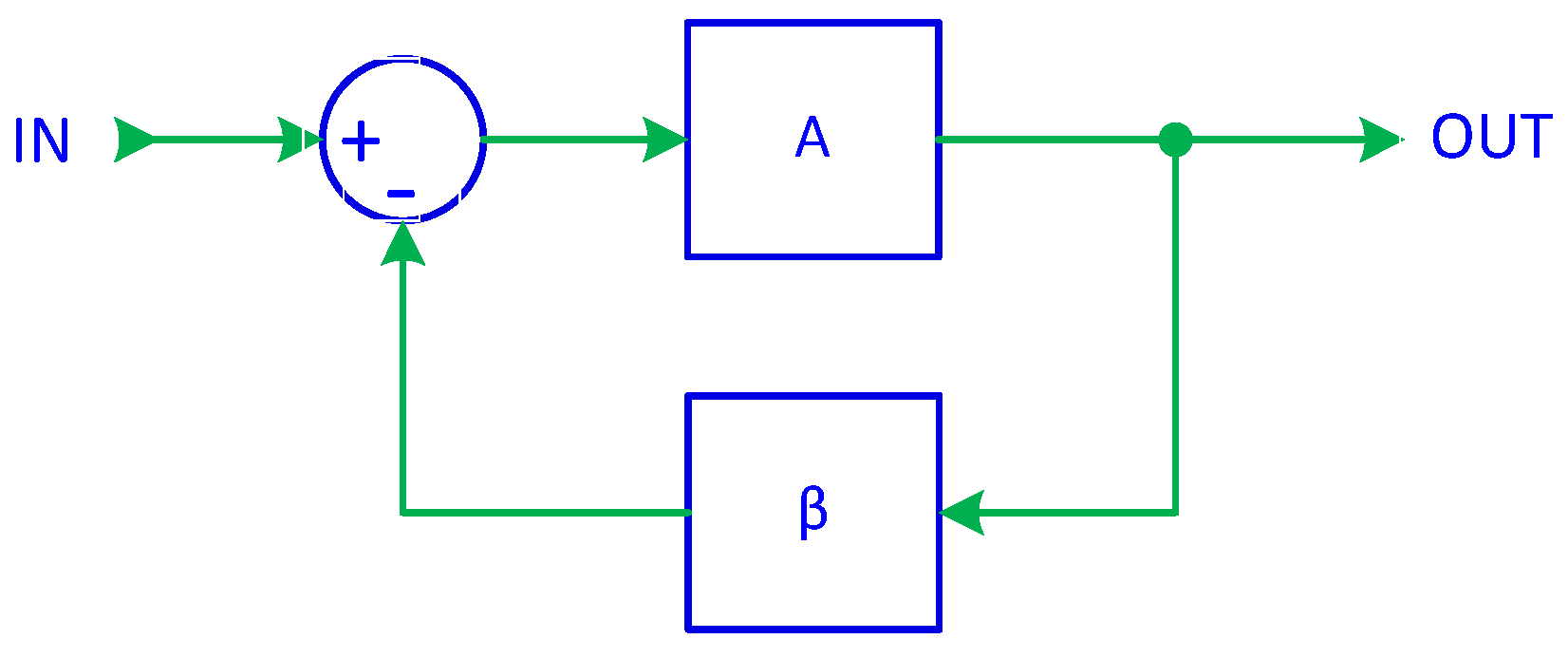
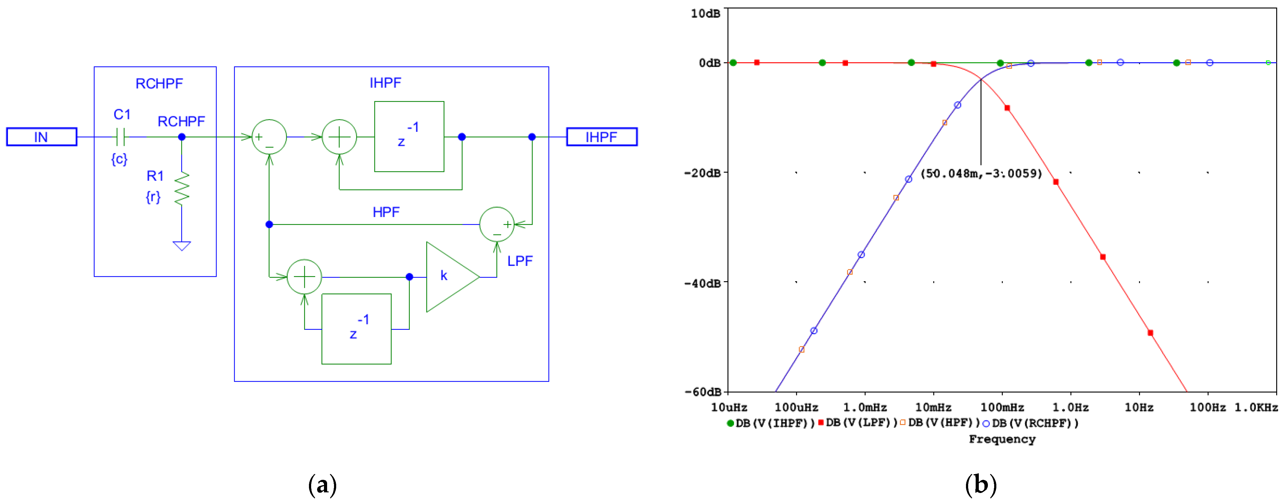
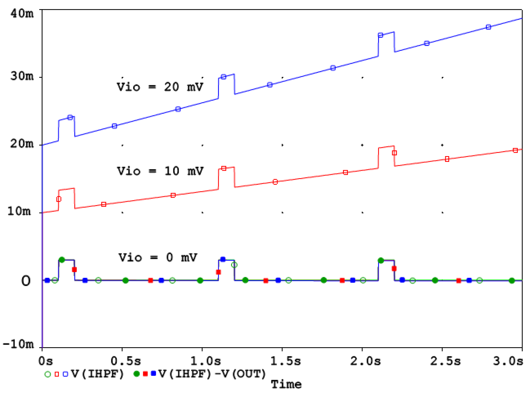
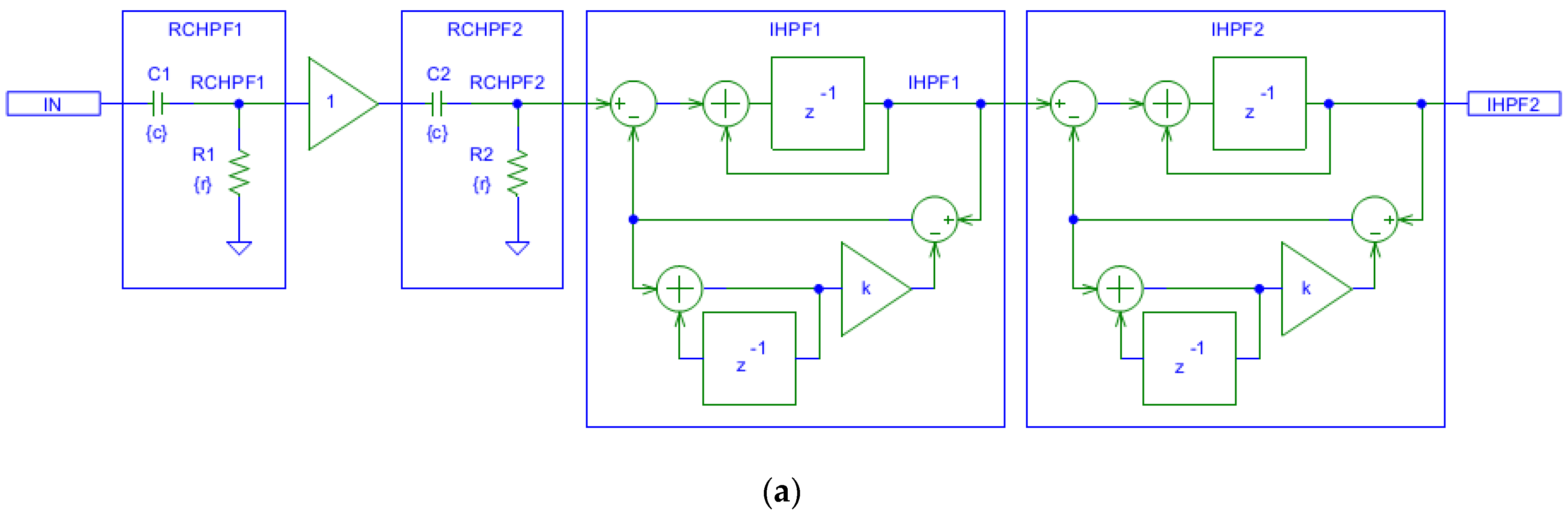
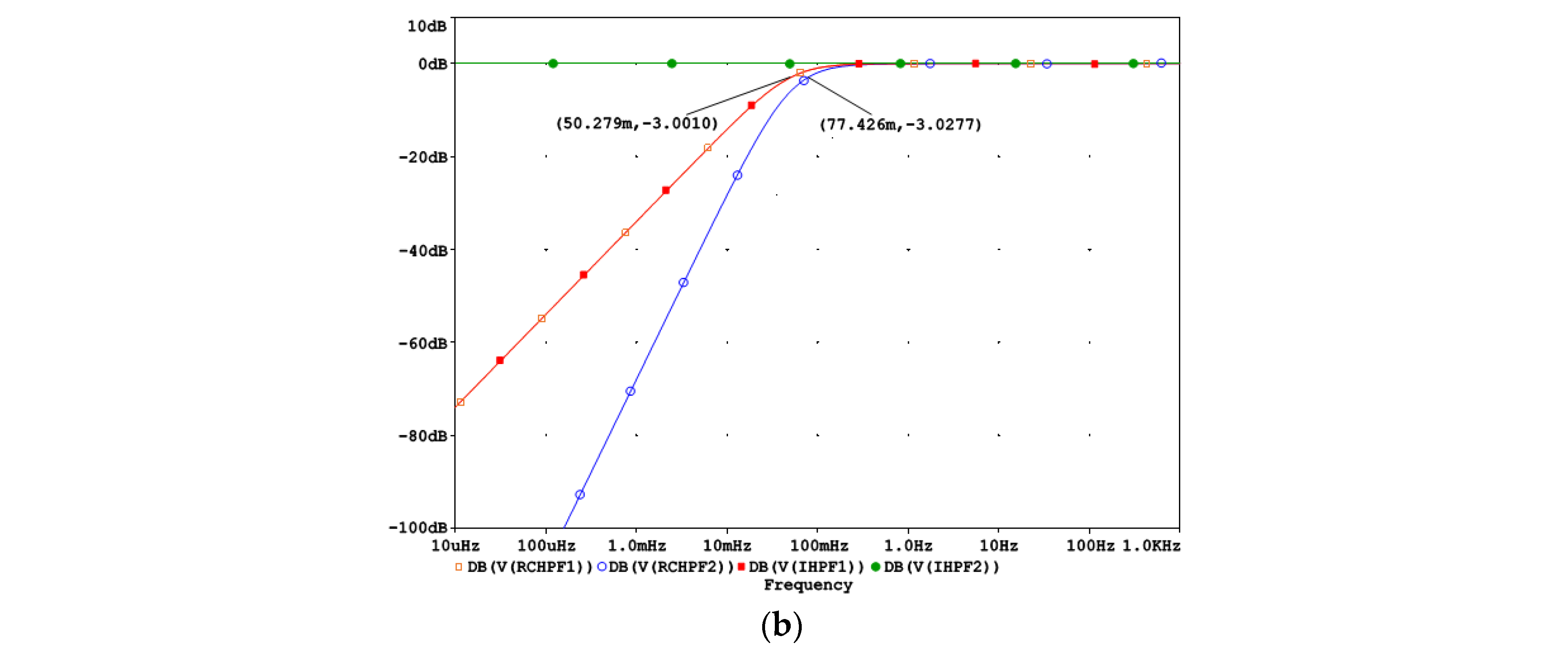
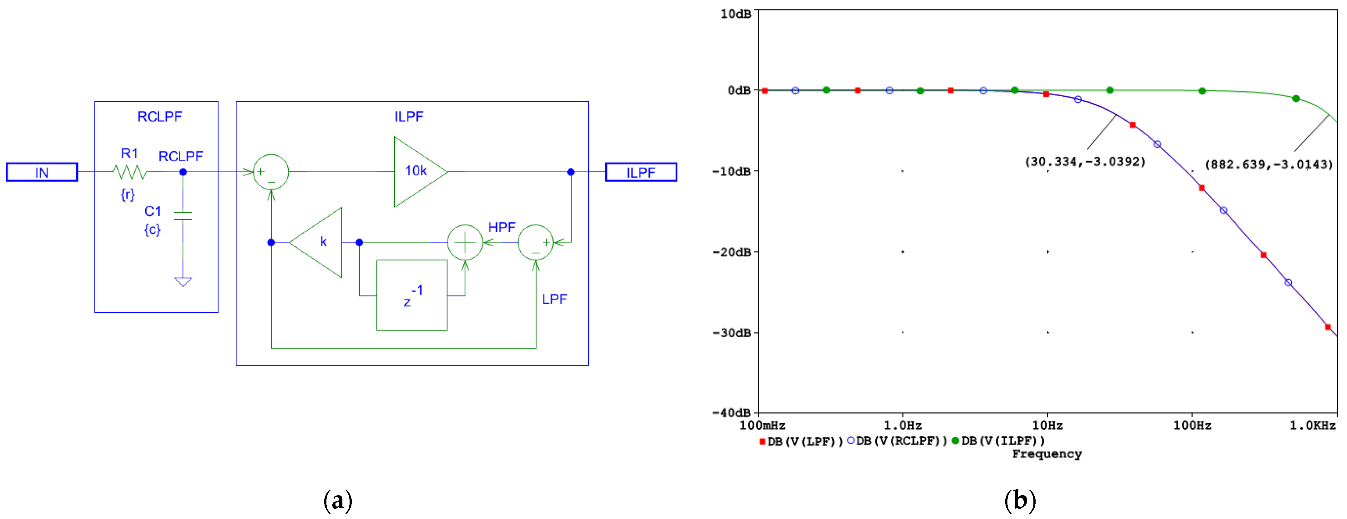
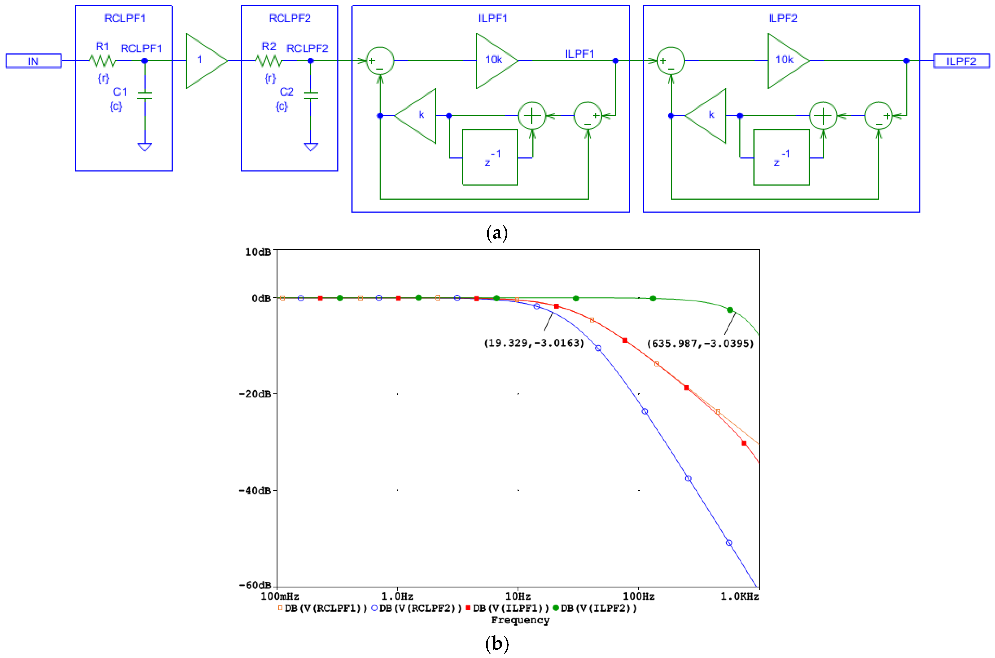
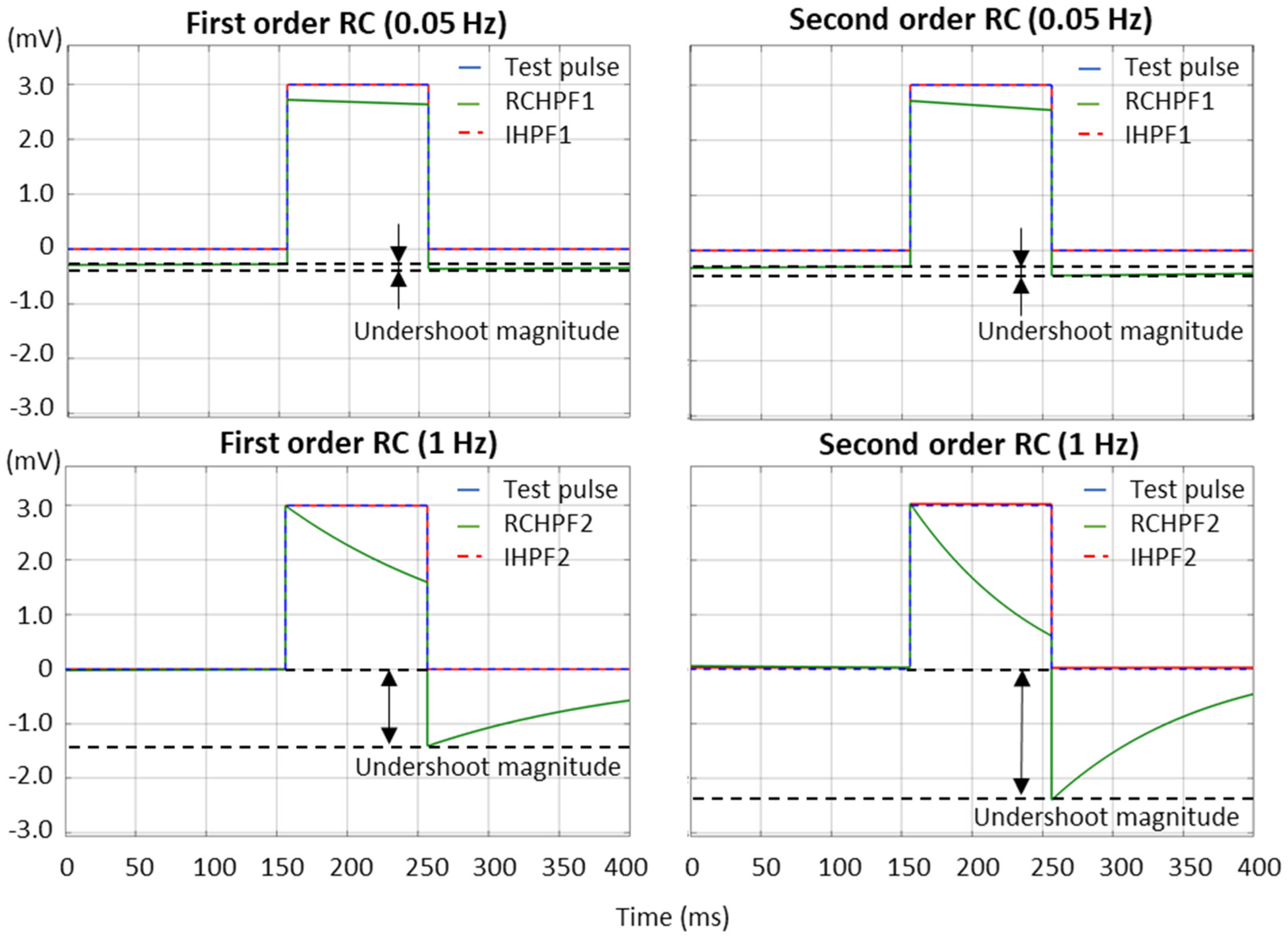
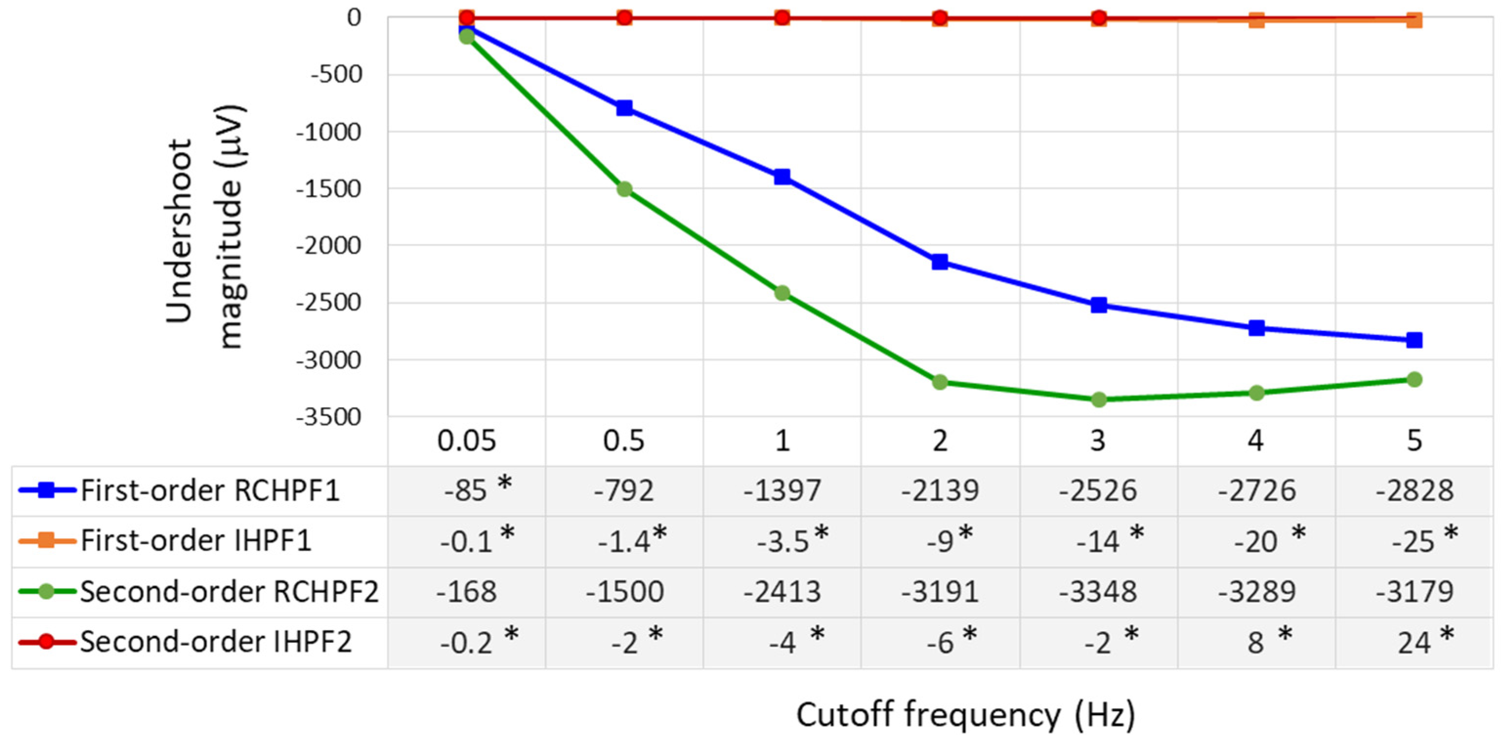
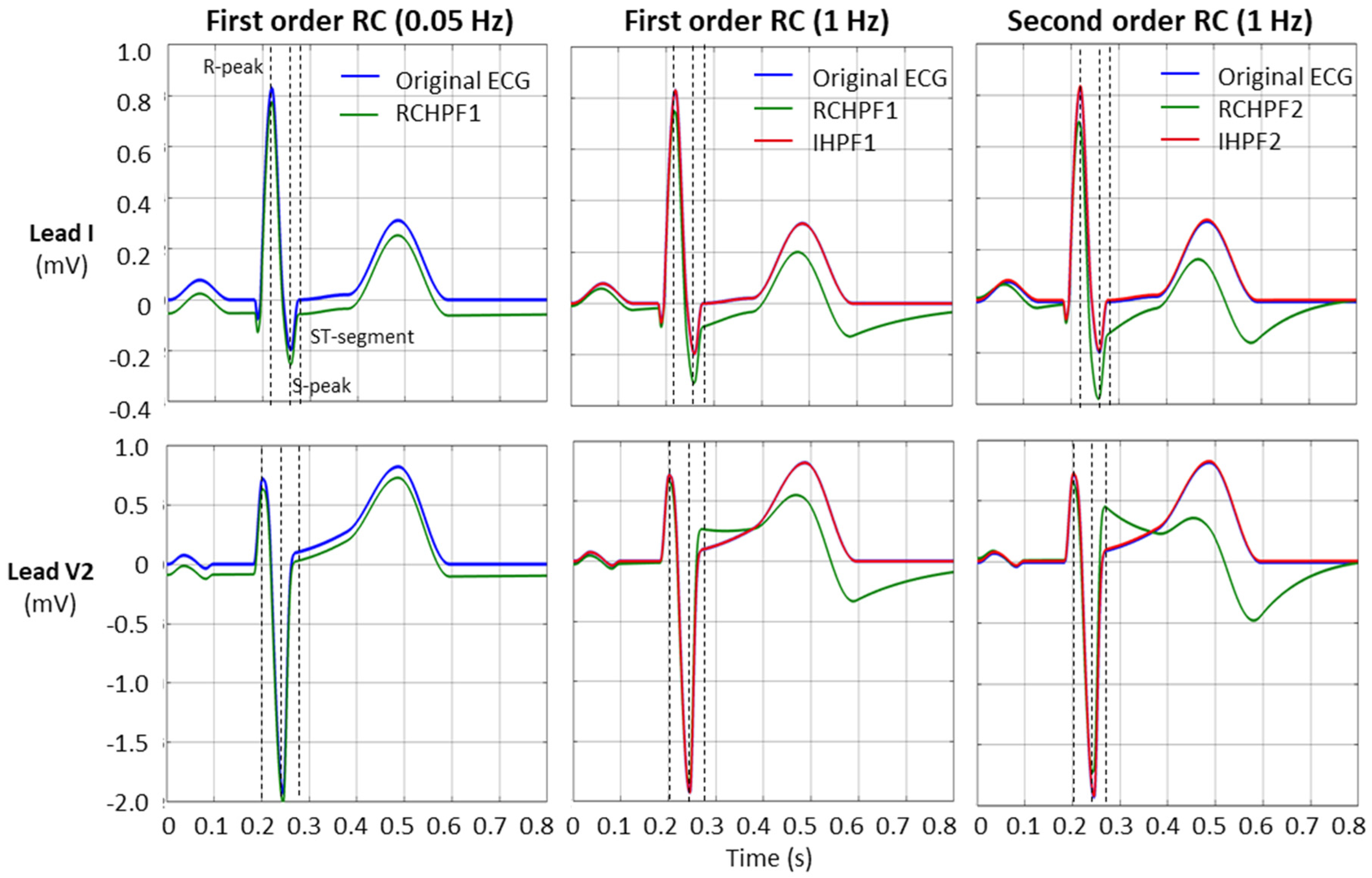
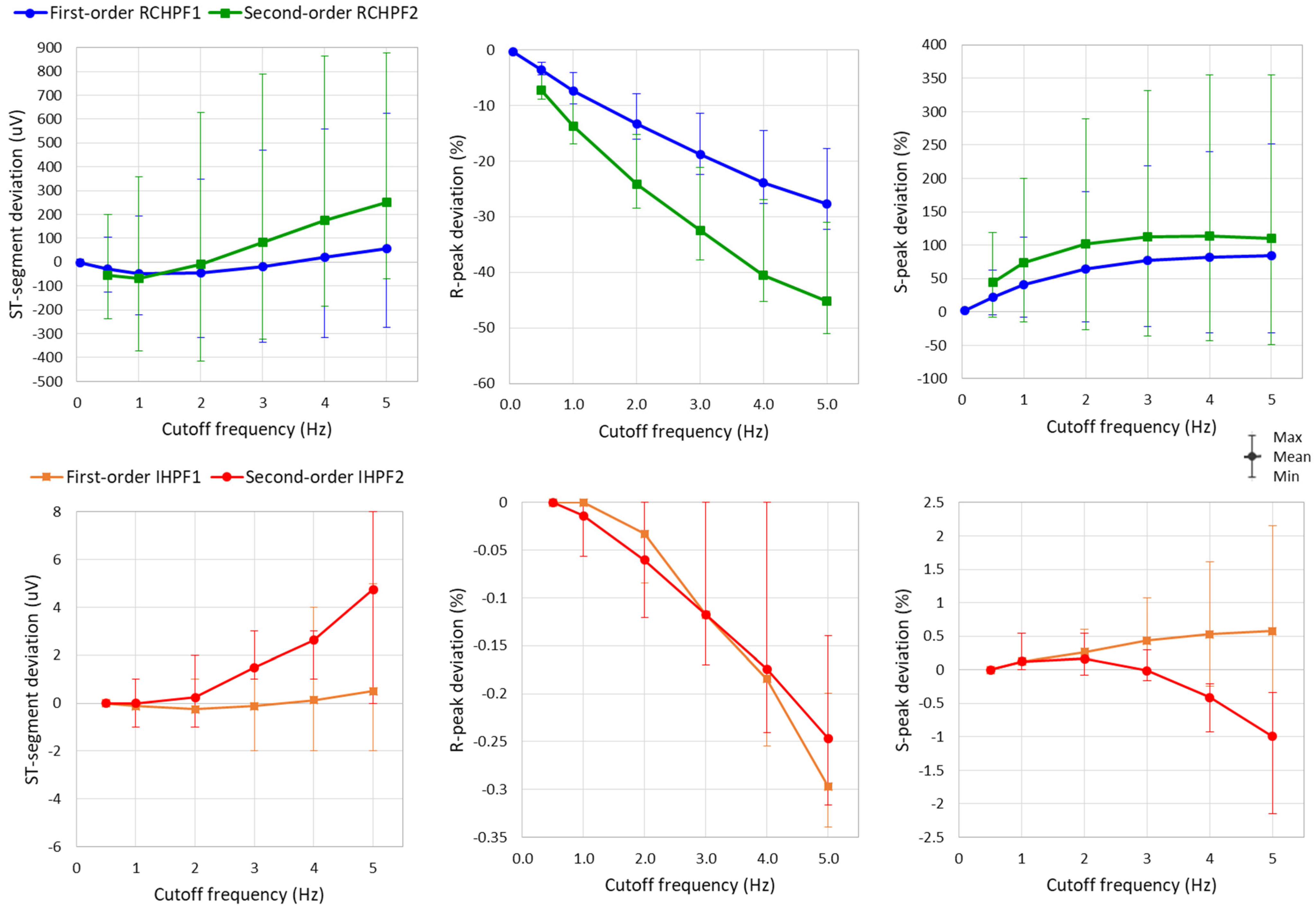
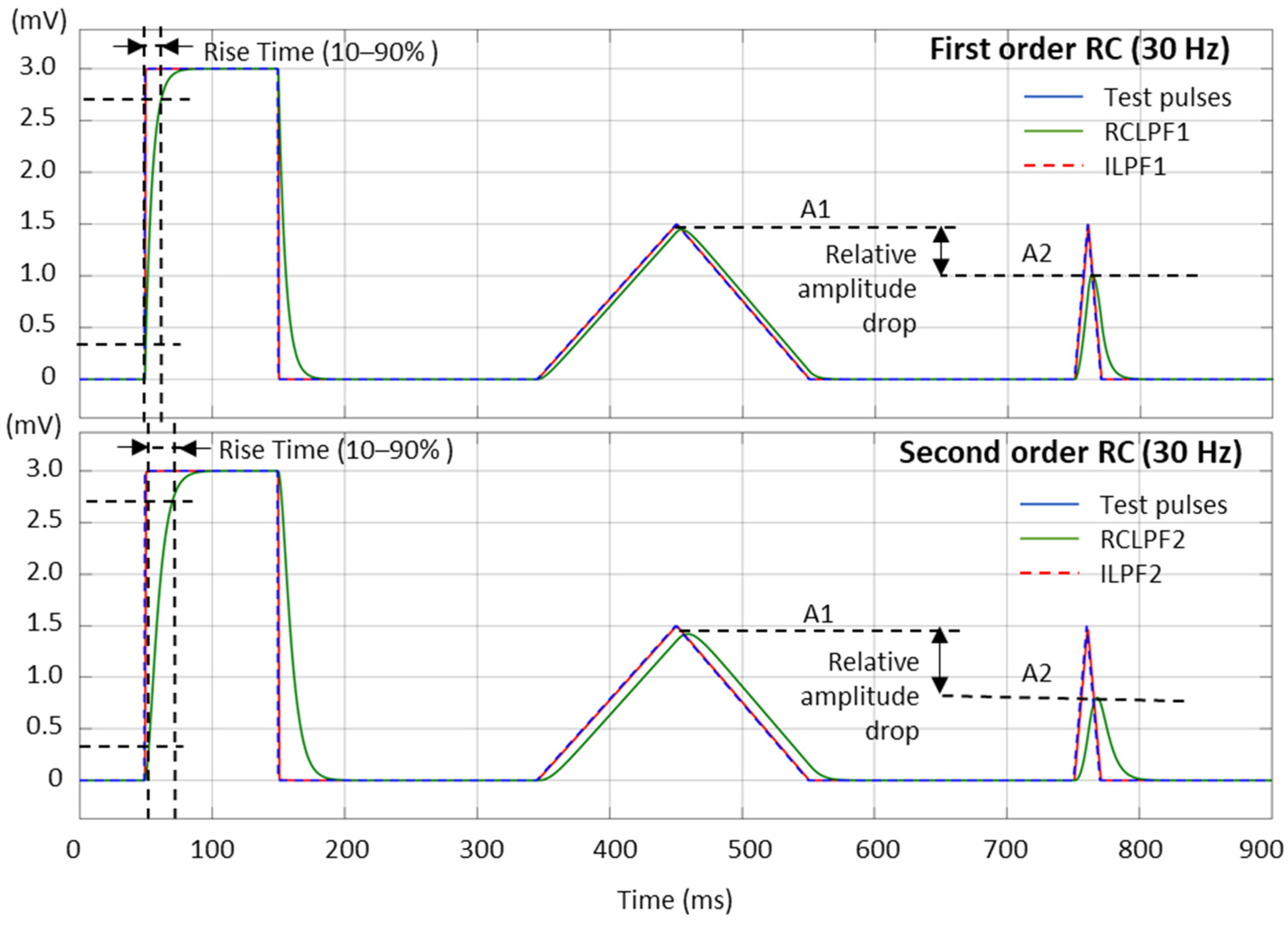
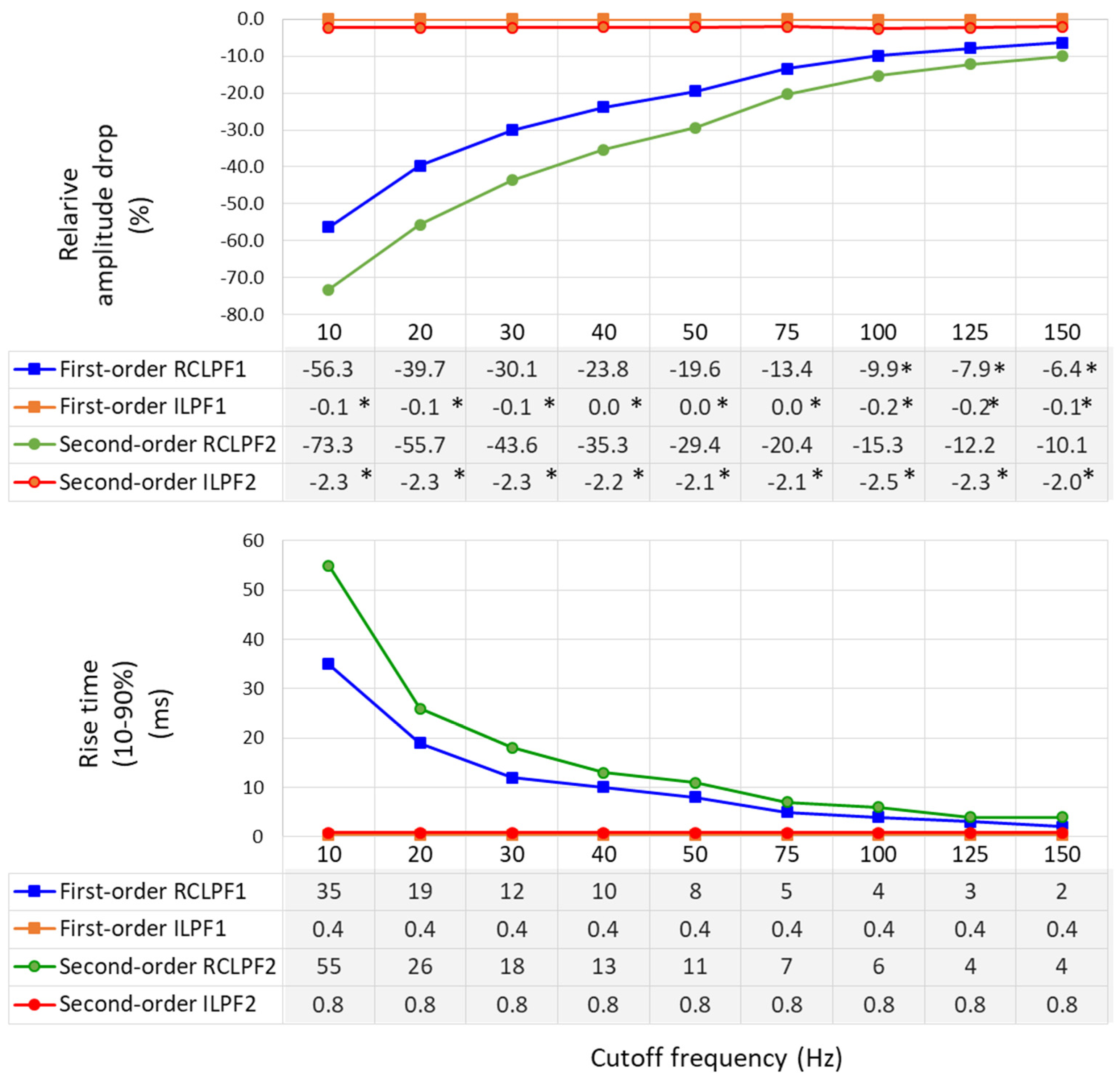
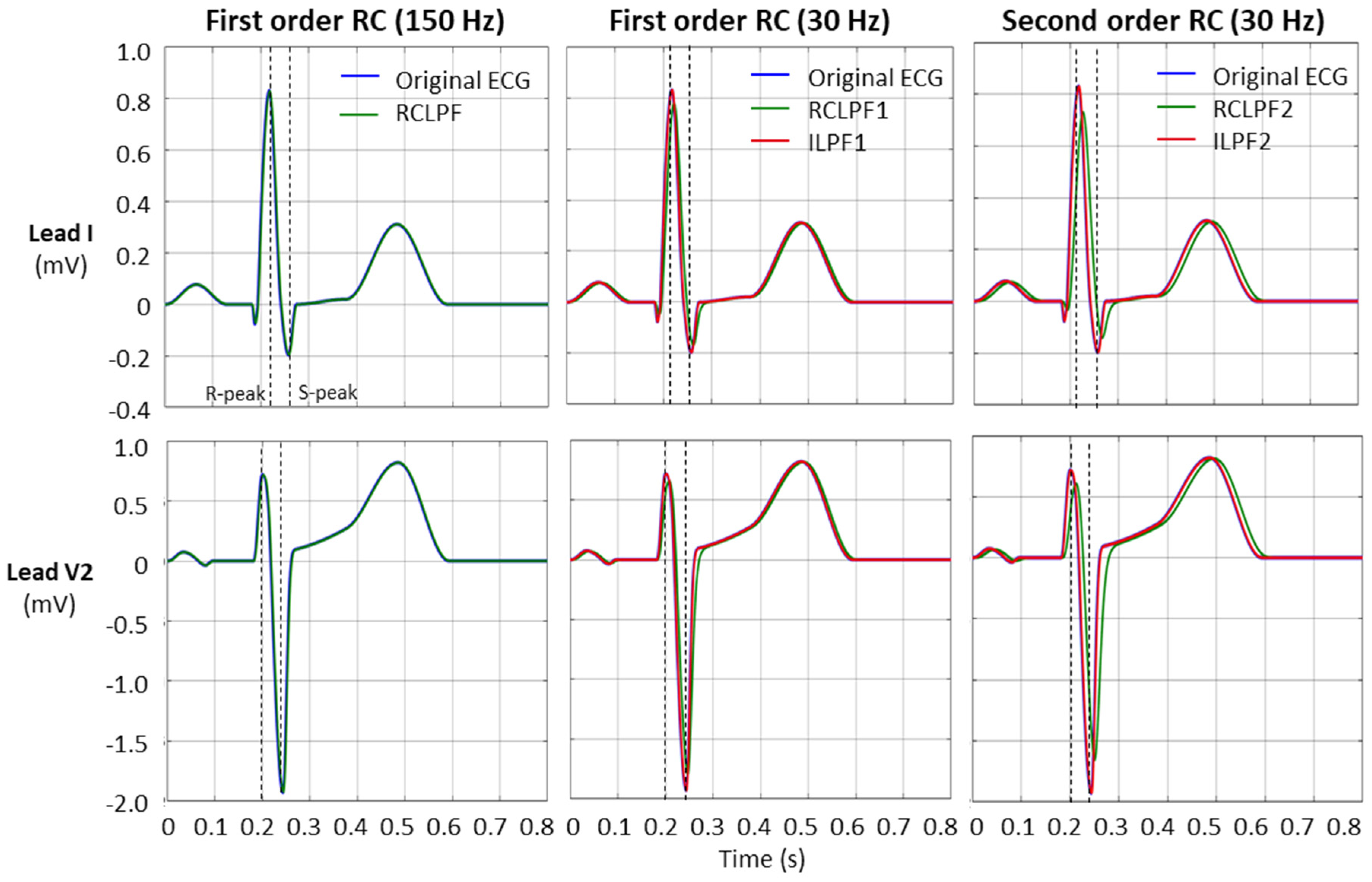
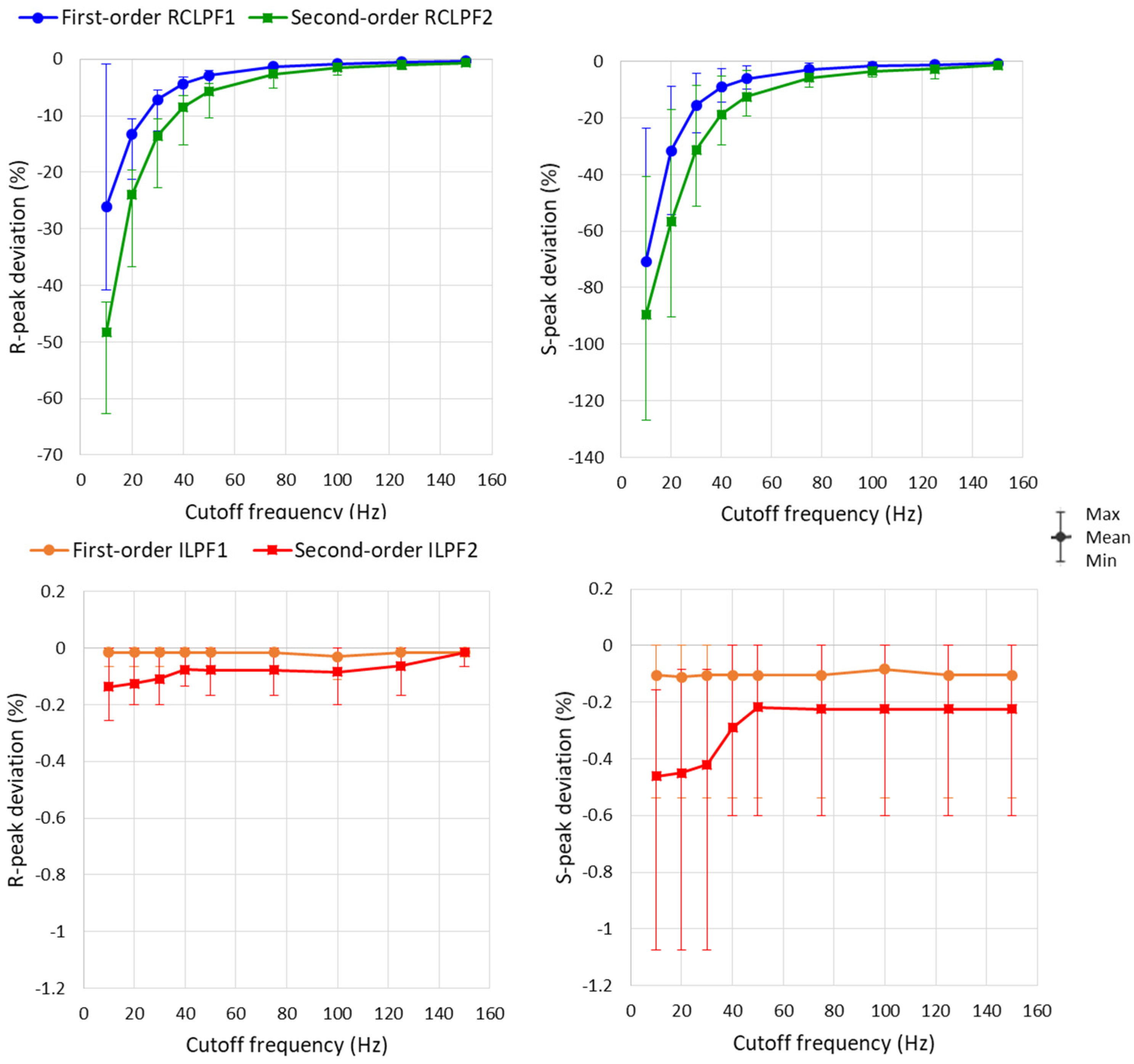
Disclaimer/Publisher’s Note: The statements, opinions and data contained in all publications are solely those of the individual author(s) and contributor(s) and not of MDPI and/or the editor(s). MDPI and/or the editor(s) disclaim responsibility for any injury to people or property resulting from any ideas, methods, instructions or products referred to in the content. |
© 2025 by the authors. Licensee MDPI, Basel, Switzerland. This article is an open access article distributed under the terms and conditions of the Creative Commons Attribution (CC BY) license (https://creativecommons.org/licenses/by/4.0/).