Abstract
The ongoing research in Environmental Scanning Electron Microscopy (ESEM) is contributed to in this paper. Specifically, this study investigates supersonic flow in a nozzle aperture under low-pressure conditions at the continuum mechanics boundary. This phenomenon is prevalent in the differentially pumped chamber of an ESEM, which separates two regions with a significant pressure gradient using an aperture with a pressure ratio of approximately 10:1 in the range of 10,000 to 100 Pa. The influence of nozzle wall roughness on the boundary layer characteristics and its subsequent impact on the oblique shock wave behavior, and consequently, on the static pressure distribution along the flow axis, is solved in this paper. It demonstrates the significant effect of varying inertial-to-viscous force ratios at low pressures on the resulting impact of roughness on the oblique shock wave characteristics. The resulting oblique shock wave distribution significantly affects the static pressure profile along the axis, which can substantially influence the scattering and loss of the primary electron beam traversing the differential pumping stage. This, in turn, affects the sharpness of the resulting image. The boundary layer within the nozzle plays a crucial role in determining the overall flow characteristics and indirectly affects beam scattering. This study examines the influence of surface roughness and quality of the manufactured nozzle on the resulting flow behavior. The initial results obtained from experimental measurements using pressure sensors, when compared to CFD simulation results, demonstrate the necessity of accurately setting roughness values in CFD calculations to ensure accurate results. The CFD simulation has been validated against experimental data, enabling further simulations. The research combines physical theory, CFD simulations, advanced experimental sensing techniques, and precision manufacturing technologies for the critical components of the experimental setup.
1. Introduction
Comprehensive research focused on the Environmental Scanning Electron Microscope (ESEM) is presented in this paper. ESEM allows for the observation of non-conductive, semiconducting, and native [1,2,3] samples without causing damage. This research is currently being conducted by a team led by Vilém Neděla at the Institute of Scientific Instruments of the Czech Academy of Sciences in collaboration with the Department of Electrical and Electronic Technology, Faculty of Electrical Engineering and Communication, Brno University of Technology. This research employs a modern approach that combines the physical theory specific to the problem with several modern types of technologies [4,5]. This involves a combination of physical theory, CFD simulations, modern experimental sensing techniques, and advanced technologies for quality control and precision of manufactured key components of the experimental setup [6,7]. In this particular case, electron microscopy was used. One aspect of this research involves investigating supersonic flow through an aperture equipped with a nozzle under low-pressure conditions at the boundary of continuum mechanics. This phenomenon is particularly relevant to the differentially pumped chamber component of the ESEM [8,9,10], which utilizes an aperture to separate two regions with a significant pressure gradient in the range of approximately 2000 Pa to 70 Pa.
The pioneer of differential pumping technology is Dr. Danilatos [11]. In his research, he focuses on the influence of nozzle geometry on system performance without an aperture. He finds that a wider nozzle opening improves electron beam transmission but can compromise the vacuum system’s pressure differential. A thinner nozzle facilitates electron beam passage but may be less effective in maintaining optimal vacuum conditions [12]. Danilatos further optimized electron beam transmission by analyzing gas density distribution [13]. He concluded that a thin nozzle reduces the pressure barrier for the electron beam. He then provided fundamental insights into the variations of density and pressure in gas flow through a small aperture separating chambers with a significant pressure difference. Using a ThermoFisher electron microscope, Danilatos investigated the impact of aperture size and controlled back pressure on gas flow [14].
Dr. Danilatos employs a fine-tuned Monte Carlo system, utilizing statistical methods for his computations. In our previous work [15], we conversely refined the Ansys Fluent system, which utilizes the continuum mechanics method based on the Stokes–Navier equations. This refinement was achieved through a comparison with Dr. Danilatos’s model from his publication of identical pressure ratios under which Dr. Danilatos performed his analysis and which are analogous to our present research.
Based on the aforementioned experience and prior research [16], the density-based model was employed, utilizing an implicit scheme, second- and third-order discretization variants, and the SST-omega turbulence model. This specific model refinement will be subsequently discussed in greater detail.
The subsequent methodological approach employed in this study utilized CFD simulations in conjunction with experimental measurements and the theoretical framework pertaining to the physical problem under investigation. A series of experimental measurements were conducted on the fabricated experimental chamber to determine the pressure ratios along the nozzle wall. These results were subsequently used to refine the CFD analyses. The refined CFD system was then applied to achieve the objective of this analysis, which was to investigate the influence of nozzle surface roughness variations on the distribution of oblique shock waves and, consequently, on the static pressure profile along the flow axis, a factor that significantly affects electron beam scattering.
The analysis of differences in flow patterns induced by nozzle roughness on the boundary layer [17], and consequently, the characteristics of shock waves, is examined in this paper. These shock waves have a significant impact on the scattering of the primary electron beam as it passes through the differentially pumped chamber, ultimately affecting the sharpness of the resulting image.
Computational Fluid Dynamics (CFD) calculations play a pivotal role in the description and analysis of supersonic flow phenomena. Specifically, they are instrumental in analyzing the distribution of shock waves, which induce abrupt changes in pressure, temperature, and density. CFD simulations facilitate a detailed investigation of shock wave formation and propagation, including their interaction with object surfaces, as will be elucidated in this paper. Consequently, CFD is frequently employed in the design and optimization of supersonic nozzles utilized in rocket engines and other related applications. These simulations enable the analysis of flow dynamics within the nozzle and the optimization of its geometry to achieve desired output flow parameters. In the present study, the objective is to minimize the axial flow pressure to reduce electron beam scattering [17,18,19,20].
However, under the operating conditions of this microscope, we are operating at the boundary of continuum mechanics in low-pressure environments. At this boundary, the ratio of inertial forces to viscous forces is significantly different [21,22]. This has a marked impact on the shaping of shock waves and their intensity [23]. In low-pressure conditions, inertial forces are significantly lower due to the reduced density. Conversely, viscous forces are largely independent of pressure up to approximately 133 Pa and do not decrease with decreasing pressure. This research is conducted using a versatile experimental chamber.
2. Experimental Chamber
This chamber is constructed from multiple components, allowing for modularity in design (e.g., nozzle shape) [24]. In particular, the chamber can be customized with various measurement devices and sensors. These sensors will primarily be used for pressure and temperature sensing. The experimental chamber is designed for the investigation of supersonic flow under significant pressure differentials between two chambers separated by an aperture and a nozzle, simulating the flow between the specimen chamber and the differentially pumped chamber.
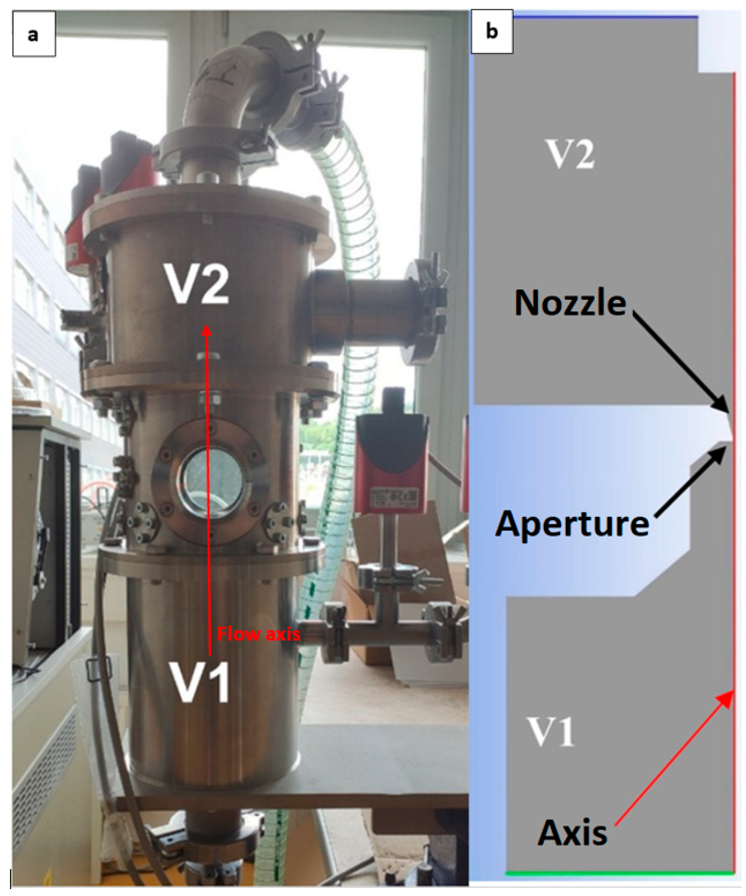
The experimental chamber consists of a chamber V1, which simulates the specimen chamber in an ESEM, and a chamber V2, simulating the conditions of a differentially pumped chamber in a real ESEM (Figure 1a). These chambers are separated by a small-diameter aperture fitted with a nozzle (Figure 1b). The modular design of the chamber allows for variations in the size and shape of both the aperture and the nozzle.

Figure 1.
Real experimental chamber (a) in conjunction with a 2D axisymmetric model of experimental chamber (b).
Additionally, the chamber is equipped with two windows, allowing for the observation of the region of interest and the visualization of shock waves using optical methods in vacuum [25,26,27]. Figure 1a presents a photograph of the chamber in conjunction with a 2D axisymmetric model (Figure 1b) on which the aforementioned CFD analyses were conducted using the Ansys Fluent system version 2024 R2.
Prior to the implementation of the 2D axisymmetric model, an analysis of the model was conducted and it was determined that the 3D effects were negligible. Subsequently, a verification simulation was performed for one variant within the 3D model, and the results were found to be consistent. Consequently, all subsequent simulations were carried out using 2D axisymmetric models. The analysis demonstrated a concordance of results while achieving a computational time reduction of up to an order of magnitude.
Two-dimensional models require significantly less computational resources than their 3D counterparts. Consequently, computational convergence is expedited and hardware demands are reduced. In complex simulations that necessitate numerous iterations or the analysis of a multitude of design variants, the utilization of 2D models facilitates substantial savings in both time and computational resources.
Given the inherent 2D nature of the system, the utilization of 2D models facilitates the deployment of a less complex mesh, thereby mitigating the risk of generating elements of suboptimal quality. This approach, in turn, reduces computational demands and curtails the potential for errors arising from compromised element integrity.
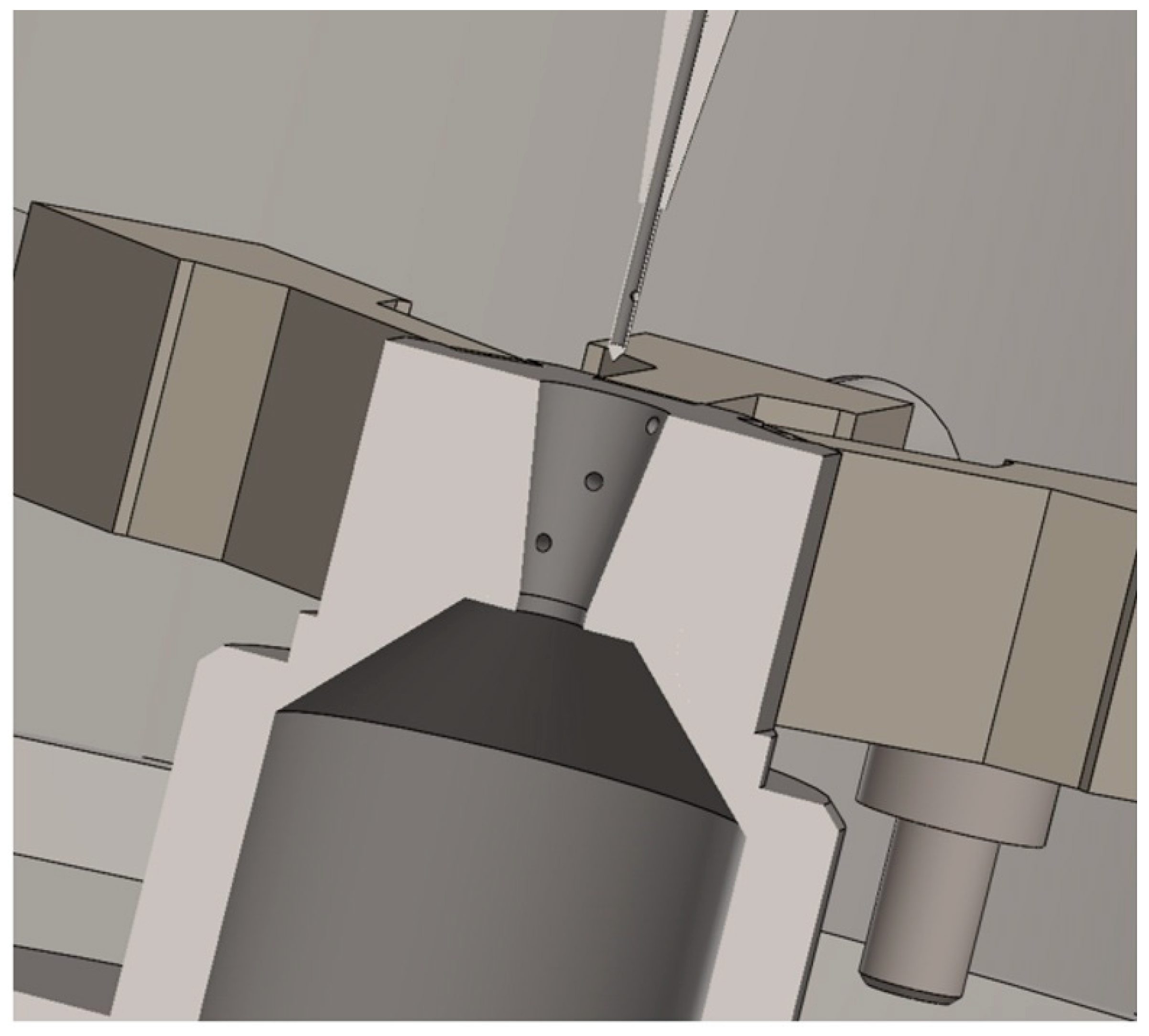
The aperture part with the nozzle is designed so that the nozzle is fitted with six spirally arranged holes on its surface. These holes can be equipped with pressure sensors to obtain the pressure distribution on the nozzle surface (Figure 2). The spiral arrangement of the holes is chosen to minimize their influence on the flow within the nozzle.
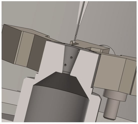
Figure 2.
More detailed view of the nozzle in 3D volume model.
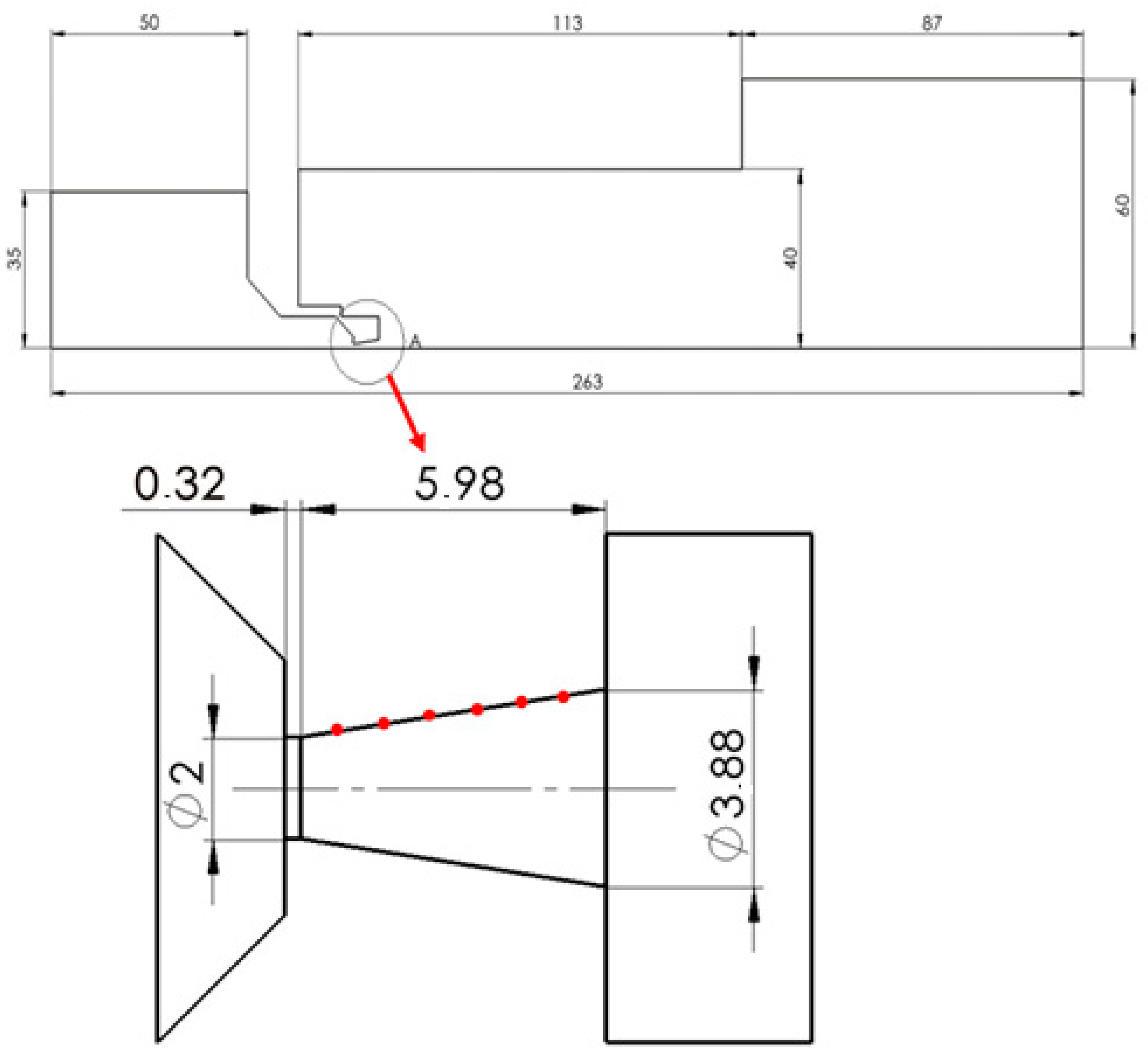
As mentioned, the CFD analyses were conducted on a 2D axisymmetric model. This 2D calculation within the Ansys Fluent system must be performed with the flow axis aligned with the X-axis. Consequently, the model needs to be rotated 90° clockwise, as illustrated in Figure 3. This figure also presents the fundamental dimensions of the CFD model, which correspond to the internal dimensions of the chamber. Moreover, the same figure displays an enlarged detail of the aperture fitted with the nozzle, including the specified dimensions and the indicated measurement points (Figure 2).

Figure 3.
Two-dimensional axisymmetric model rotated 90° with the dimensions of the given model and points for sensing (red points).
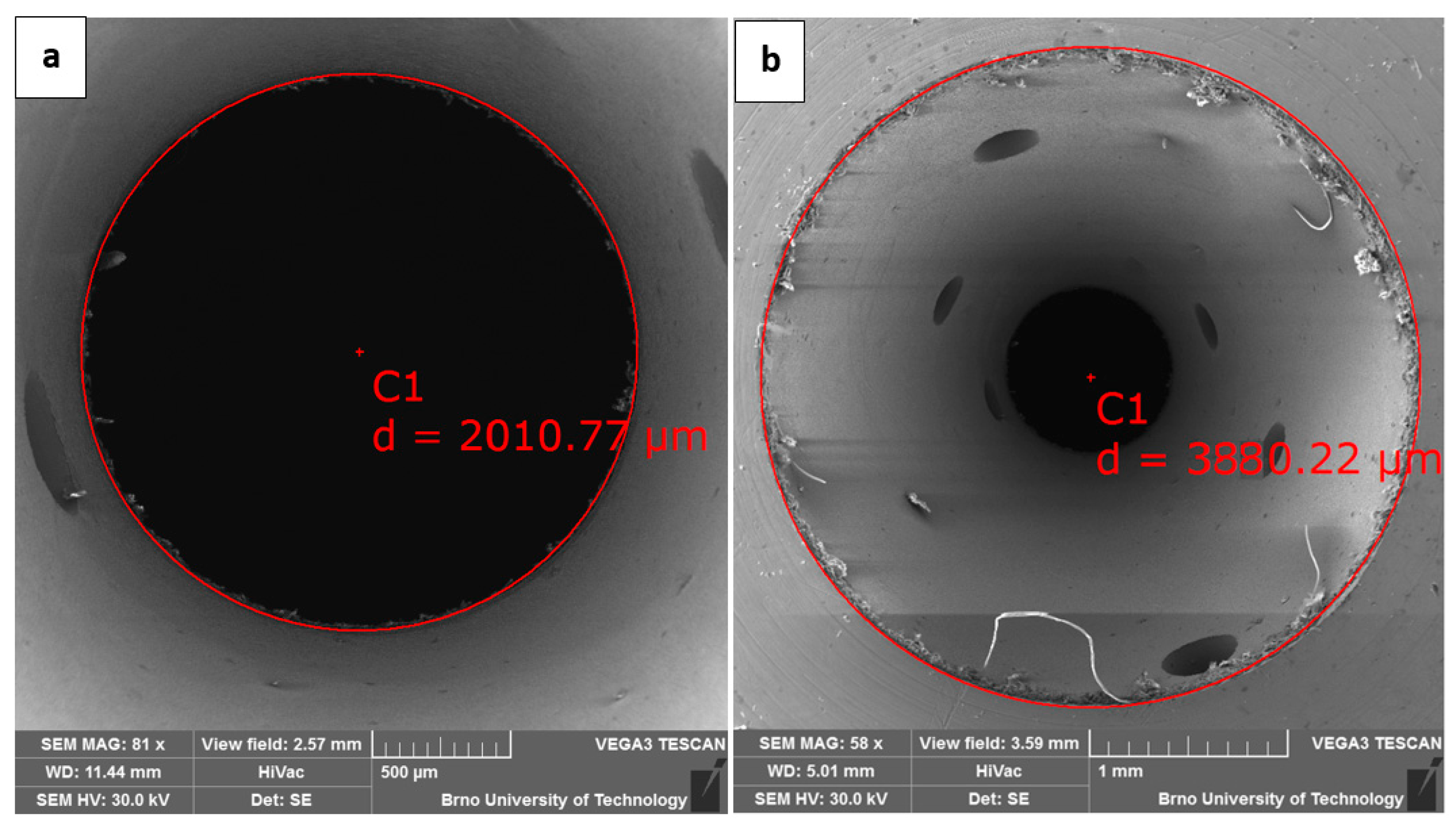
The nozzle dimensions were adjusted in CFD model to match those of the actual manufactured nozzle within the specified tolerance (Figure 3). The dimensions of the manufactured nozzle were analyzed using the VEGA3 Tescan (Brno, Czech Republic) optical microscope (Figure 4). Subsequently, CFD analyses were conducted using these dimensions of the actual manufactured nozzle. The residues visible in Figure 4 were cleaned up.
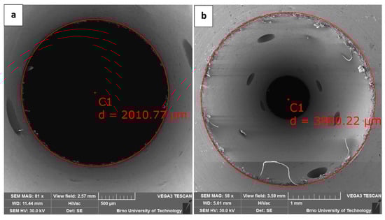
Figure 4.
Real dimensions of aperture (a) and nozzle outlet (b).
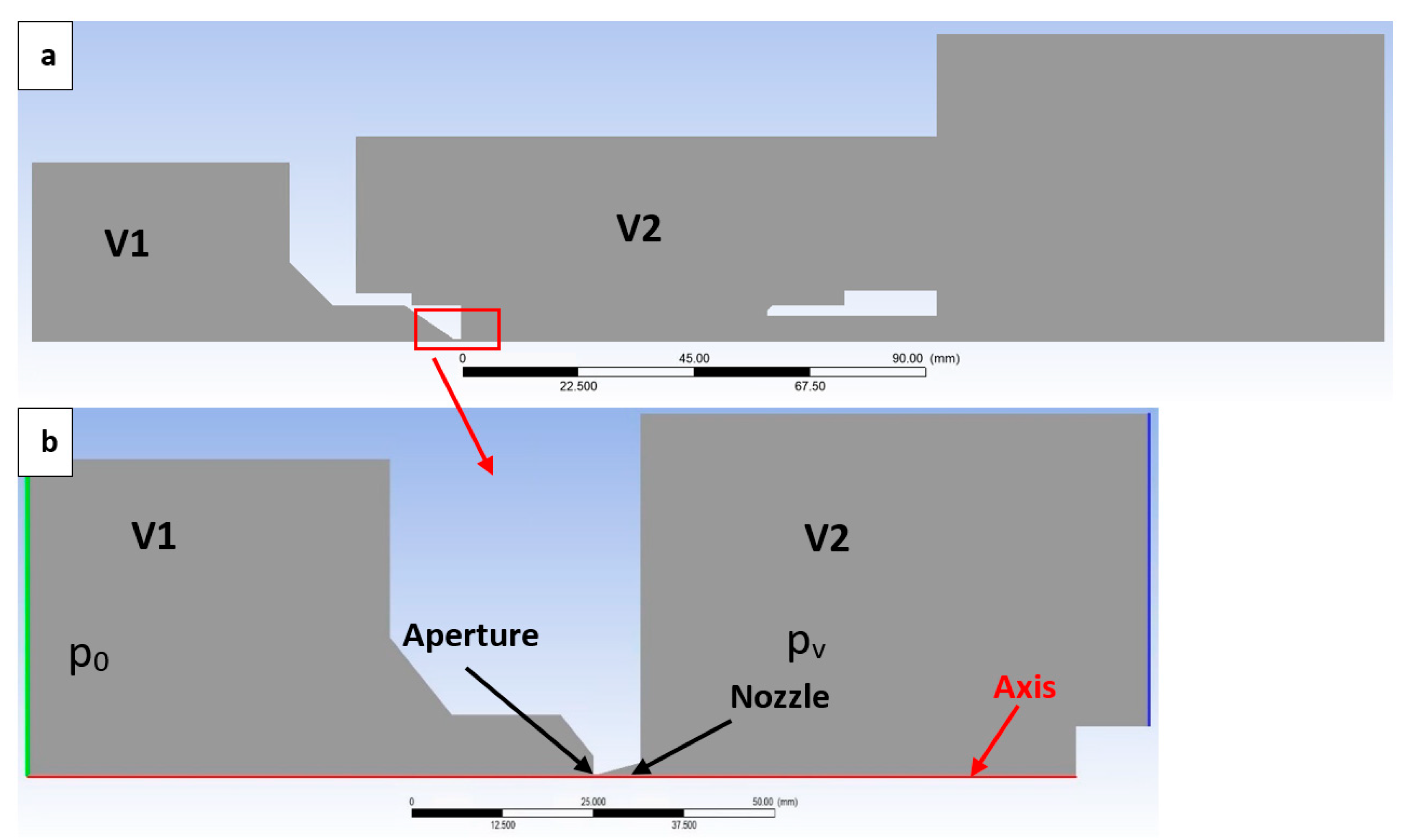
Figure 5 presents a 2D axisymmetric model for CFD analysis, including a description of the boundary conditions. Two variants with very similar pressure gradients were analyzed. The first variant was tuned for atmospheric conditions: p01 = 1,013,250 Pa: pv1 = 101,325 Pa (hereafter referred to as the ATM variant). The second comparative variant was designed for conditions close to the continuum mechanics limit: p02 = 13,947 Pa: pv2 = 1158 Pa (hereafter referred to as the 1158 Pa variant). As previously mentioned, chamber V1 denotes the chamber behind the aperture, while V2 represents the chamber into which the gas flows through the aperture and nozzle.

Figure 5.
Two-dimensional axisymmetric model of chambers for CFD analysis (a) with zoomed area with labeled boundary conditions (b).
3. Methodology
The methodology employed in this paper is based on a combination of experimental measurements and CFD analyses [28,29]. The experimental measurements consisted of a series of strategically placed pressure sensors. The CFD analyses were performed using the Ansys Fluent system, employing the finite volume method within the framework of continuum mechanics [30].
Initially, a CFD analysis was performed using Ansys Fluent system. Based on the predicted pressures at the pressure measurement points on the nozzle wall, differential pressure sensors were selected. These sensors were chosen with the narrowest possible measurement ranges to achieve the highest measurement accuracy [31].
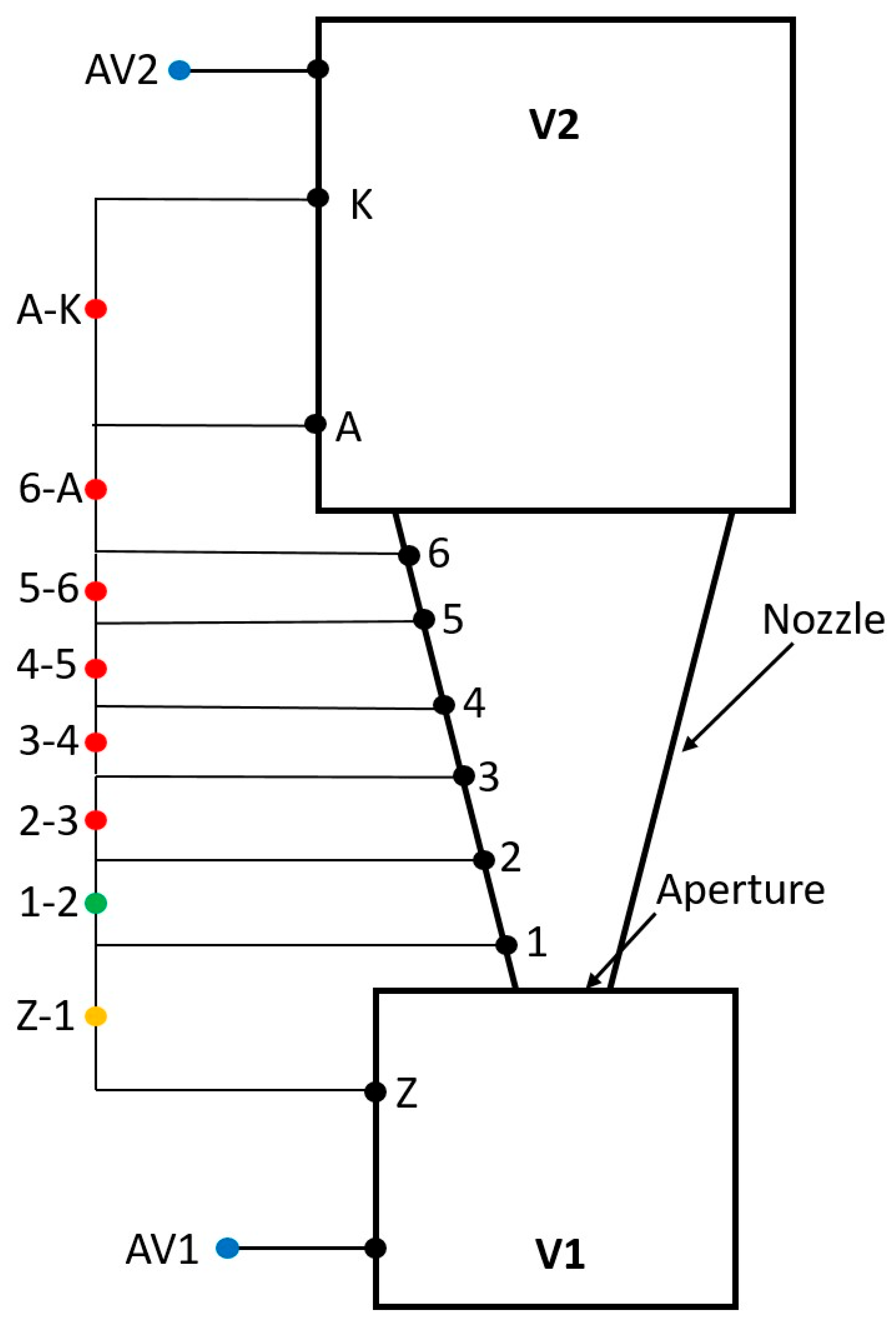
Figure 6 presents a schematic diagram of the experimental chamber, illustrating the schematic arrangement of the pressure sensors (the dimensions are not proportional). Point AV1 was measured using an absolute pressure sensor, the Pfeiffer CMR 361, with a range of 110 kPa and an accuracy of ±0.2% of the measured value. Point AV2 was measured using an absolute pressure sensor, the Pfeiffer CMR 362, with a range of 11 kPa and an accuracy of ±0.2% of the measured value. The differential pressure between points Z and 1 was measured using a DPS 300 sensor with a range of 100 kPa and an accuracy of ±1% FSO BFSL (over the entire range fitted with a linear curve). The differential pressure between points 1 and 2 was measured using a DPS 300 sensor with a range of 25 kPa and an accuracy of ±1% FSO BFSL (over the entire range fitted with a linear curve). The differential pressure between points 2 and 3 was measured using a DPS 300 sensor with a range of 4kPa and an accuracy of ±1% FSO BFSL (over the entire range fitted with a linear curve). The differential pressure between points 3 and 4 was measured using a DPS 300 sensor with a range of 400 Pa and an accuracy of ±1% FSO BFSL (over the entire range fitted with a linear curve). The differential pressure between points 4–5, 5–6, 6–A, and A–K was measured using a DPS 300 sensor with a range of 160 Pa and an accuracy of ±1% FSO BFSL (over the entire range fitted with a linear curve).
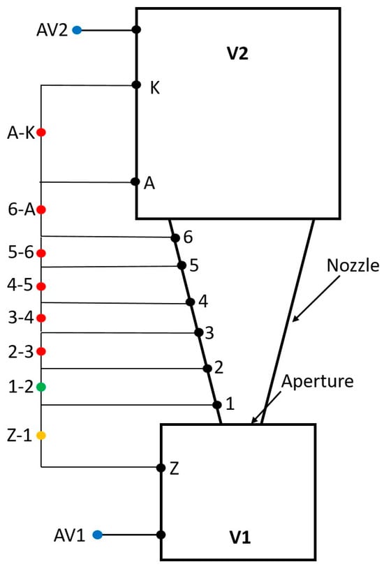
Figure 6.
Schematic arrangement of the pressure sensors.
Subsequently, experimental pressure measurements were conducted on the nozzle surface. This was carried out using pressure sensors installed in the experimental chamber configured for the 1158 Pa variant. The measurement setup is depicted in Figure 6. The experimental data were then validated against the results obtained from the CFD analyses, leading to the fine-tuning of the Ansys Fluent model.
Due to the high compressibility of supersonic flow, it is imperative to employ models that account for density variations within the flow field. The Ansys system utilizes two fundamental models with the provision for further customization.
The pressure-based coupled solver, which simultaneously solves the momentum and continuity equations, updates the pressure and velocity fields concurrently at each iteration. Conversely, the density-based solver is designed to accurately model density variations, thus solving the continuity, momentum, and energy equations in their compressible forms. It predominantly employs “implicit” solution methods, which exhibit enhanced stability for compressible flows characterized by shock waves.
When selecting among the given solvers, the decisive criterion is not so much the magnitude of velocity, but rather the consideration of inertial effects in cases where the coupling between the momentum and energy equations is strongly nonlinear. These nonlinearities influence the resulting behavior. While the pressure-based solver suppresses inertial effects and linearizes the coupling between the momentum and energy equations, the density-based solver has an advantage in this regard. The selection should be made based on whether these effects need to be included in the analysis.
In simplified terms, when simulating shock waves and analyzing the influence of inertial effects, a pressure-based solver can be employed up to a flow velocity of 0.3 Mach. If these effects are not required to be included, the pressure-based solver can yield satisfactory results for compressible fluids, even at flow velocities of 3 Mach.
For the aforementioned reasons, the density-based solver was chosen as the most suitable option due to the complex flow dynamics within the nozzle. This solver simultaneously solves the density-based equations for continuity, momentum, energy, and substance transport, while other scalar equations are solved sequentially.
To handle the intricate flow patterns, an implicit linearization approach was used for solving the conjugate equations. This method linearizes each equation implicitly with respect to all dependent variables. The pooled implicit approach, which solves all variables across cells simultaneously, proved to be stable and effective for handling the complex supersonic flow conditions and significant pressure differentials encountered in the experiments.
Due to the supersonic nature of the flow, the equation of friction dissipation was included in the energy equation.
For the numerical scheme, we chose AUSM (Advection Upstream Splitting Method) [32]. This advanced method formulates convective and compressive flows using the eigenvalues of the Jacobian flow matrices. The AUSM scheme offers several advantages:
- Accurate representation of shock and contact discontinuities.
- Entropy-conserving solutions.
- Elimination of the “carbuncle” phenomenon, a numerical instability often seen in low-dissipative techniques.
- Consistent accuracy and convergence rates across all Mach numbers.
The AUSM scheme demonstrates applicability across a broad spectrum of Mach numbers, encompassing both low subsonic and high supersonic velocities. AUSM is capable of delivering accurate results even in subsonic regimes, where alternative numerical discretization methods are frequently susceptible to numerical errors. Furthermore, it exhibits robust behavior in the transonic region, where flow transitions from subsonic to supersonic. For supersonic velocities, AUSM is designed to accurately capture shock waves and other discontinuities encountered at elevated Mach numbers. Consequently, AUSM proves to be a suitable choice for supersonic and hypersonic flow simulations.
The AUSM scheme minimizes numerical dissipation, resulting in enhanced accuracy, particularly in flows exhibiting sharp gradients, and demonstrates robust shock-capturing capabilities, which are crucial for supersonic and hypersonic flow simulations.
To transfer data between cells, we used a second-order upwind scheme. This scheme utilizes a technique called ‘multivariate linear reconstruction’ to calculate values on cell surfaces. It essentially takes the cell-centered data and uses mathematical expansion (similar to a Taylor series) to create a more accurate representation of the values at the cell faces [33,34,35]. This approach helped us to capture the dynamic flow changes during pumping and produced results that closely matched our experimental measurements. Since a precise mathematical analysis was also crucial, we carefully designed the mesh beforehand [36,37].
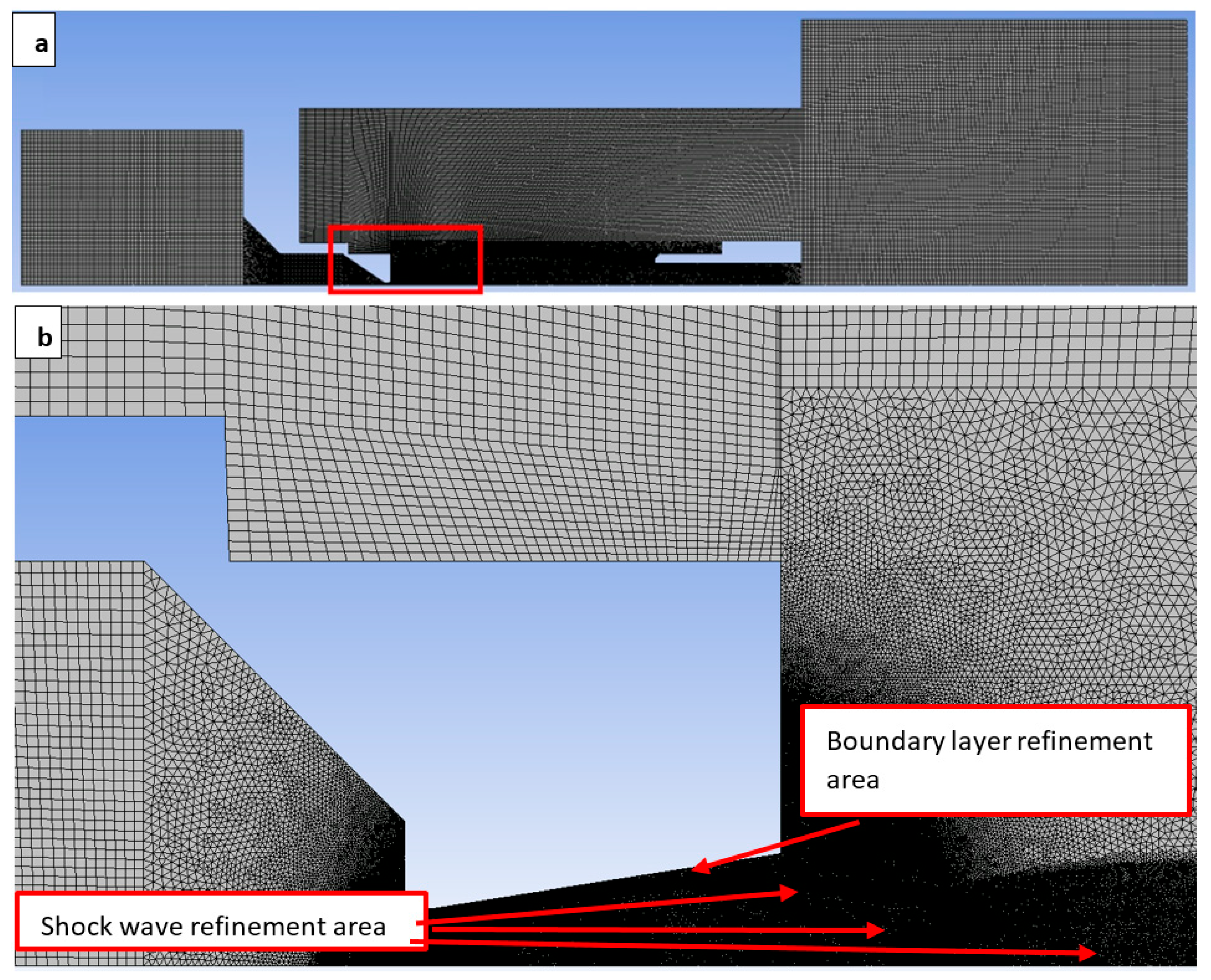
A structured mesh combined with a 2D variant of hexagonal elements was used, offering advantages such as reduced artifacts from transmitting results over oblique edges and a minimized cell count for purely rectangular regions (Figure 7a). Triangular elements were employed in areas where a structured mesh was impractical, notably in narrow sections like the nozzle aperture and regions with anticipated supersonic flow behind the nozzle. Particular attention was paid to modeling a sufficiently fine boundary layer in this aperture and nozzle [38].
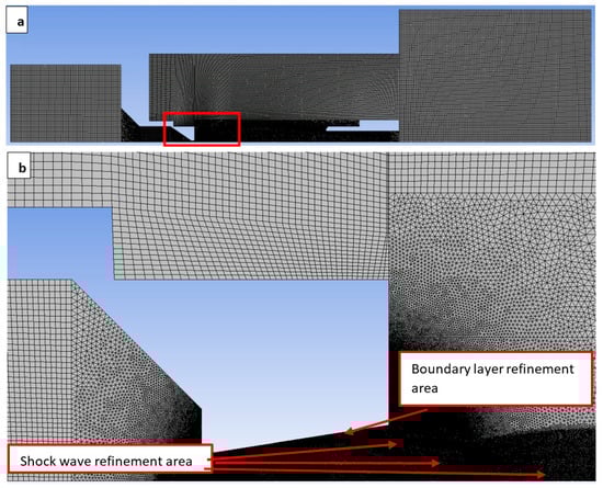
Figure 7.
Structured mesh for the CFD analysis (a) with zoomed area with the mesh refinement (b).
Figure 7b illustrates an expansion of the rectangular area (Figure 7a). The zoomed-in portion highlights the pre-planned refinement. Manual adaptive refinement was also implemented during the calculation process using the Field Variable method according to the pressure gradient. Refinement was performed in regions where oblique and normal shock waves were formed [39].
Ansys Fluent employs unstructured mesh (specifically, triangular elements in 2D) for adaptive refinement, primarily due to the mesh’s inherent flexibility. In adaptive refinement procedures, localized mesh modifications are necessitated based on computational results, a process that can be exceedingly complex with structured meshes. Unstructured meshes facilitate a more straightforward and automated refinement process in regions characterized by steep gradients, such as shock waves or turbulent flows.
The range of mesh adaptation was determined based on the maximum values of the gradient of pressure in the cells. The maximum refinement level was set to 4 to accurately capture pressure gradients in the supersonic flow regions within the nozzle. A grid independence study was conducted. Manual mesh adaptation was applied across the pressure range, with a refinement level of 2 used in areas with minimal variable changes. Areas preceding the aperture within the nozzle and in the gas expansion zone were refined to a maximum level of 4. Throughout the calculation process, the monitoring setup in Ansys Fluent remained unchanged. Global parameters such as Absolute Pressure, Static Temperature, Velocity, and Density were continuously monitored. Parameter Points were established at specific locations: within the aperture throat and at five points spaced 2 mm apart in the direction of gas flow above the aperture. The subsequent evaluations of quantities, as detailed later in the paper, exhibited consistency. The grid independence analysis confirmed that the mesh resolution was adequate for the type of analysis conducted.
The CFD results were subsequently utilized to verify the boundary layer conditions by examining the y+ value [40,41]. The initial cell size near the wall, especially in the boundary layer of the aperture and nozzle, was critical for creating the mesh. The SST k-ω turbulence model was employed, assuming a y+ value between 0 and 1. The size of the first cell next to the wall can be calculated using Equation (1).
where y+ is dimensionless quantity that represents the distance from the wall within the boundary layer, scaled according to the flow characteristics, μ is dynamic viscosity, and Uτ is frictional velocity.
The k-ω turbulence model used does not have a built-in mathematical wall function model. This means that the y+ value must be less than 1. To accurately represent the boundary layer, the mesh needs to be fine enough in this area, and the first cell near the wall should be small [42].
The dynamic viscosity, which changes based on the gas temperature T, is calculated using Equation (2) [43] and verified according to [44]. This is especially important in supersonic flow where viscosity changes significantly.
The frictional velocity Uτ is determined from Equation (3):
where is wall shear stress determined from Equation (4):
where Umax is maximal gas flow velocity in the flow axis, and Cf is skin friction coefficient.
The skin friction coefficient is a dimensionless number that measures how much friction a flowing fluid exerts on a surface compared to its dynamic pressure. It is calculated using Equation (5):
where is Reynold number obtained from Equation (6):
where D is characteristic dimension of internal solved space and Umid is mean flow velocity.
The mean flow velocity Umid in the cross-section of the given nozzle was determined from Equation (7):
These relationships were subsequently utilized in the evaluation of individual calculation variants.
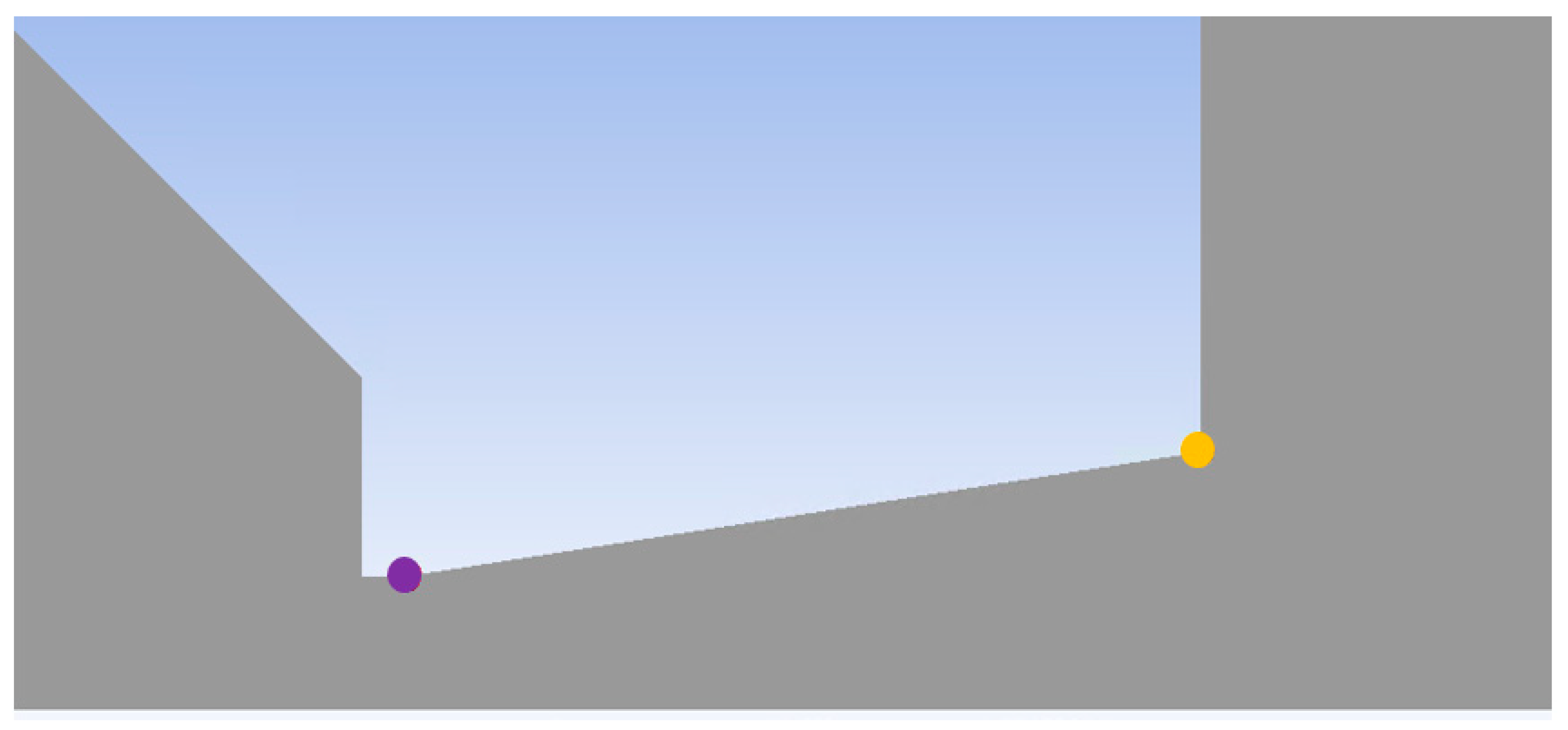
The y+ value was verified according to the theory described above. The required maximum size of the first cell at the wall was determined at two locations: the aperture throat (purple point) and the nozzle outlet (yellow point) (Figure 8). Table 1 shows the results of the first cell size y in the given points. The remaining quantities presented in Table 1 were obtained from CFD analyses conducted using Ansys Fluent.
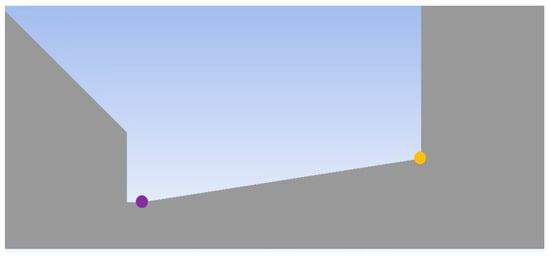
Figure 8.
Locations for y+ verification at nozzle throat (purple point) and nozzle outlet (yellow point).

Table 1.
Results of the first cell size y in the given points.
The mesh was constructed with the careful consideration of the acquired data. The calibrated CFD model was then used to analyze the ATM variant, and the resulting flow patterns were compared to those of the 1158 Pa variant, revealing significant differences in boundary layer behavior.
A boundary layer is a thin region of fluid that forms near a solid surface when a fluid flows over it. Due to the no-slip condition, the fluid velocity at the surface is zero. The fluid velocity gradually increases with distance from the surface until it reaches the free-flow velocity. Boundary layers significantly influence drag, heat transfer, mass transfer, and turbulence. The boundary layer can be either laminar or turbulent. Laminar boundary layers exhibit smooth, orderly flow with minimal mixing between fluid layers and are typically found near the leading edge of an object or at low Reynolds numbers. Turbulent boundary layers, on the other hand, are characterized by chaotic, irregular flow, with significant mixing, and occur at higher Reynolds numbers, usually downstream of the laminar region. Boundary layer thickness is defined as the distance from the surface at which the fluid velocity reaches approximately 99% of the free-flow velocity. This thickness is influenced by factors such as flow velocity, fluid viscosity, and the length of the surface over which the fluid flows.
In electron microscopy, the interaction between the electron beam and gas molecules results in the scattering of primary electrons. The operation of electron microscopes designed for higher chamber pressures, specifically Environmental Scanning Electron Microscopes (ESEM), is predicated on the phenomenon that a portion of the electron beam retains its original trajectory even after traversing a gaseous medium.
The passage of a primary electron beam through an environment with elevated gas pressures results in collisions between the electrons and gas atoms and molecules. During these collisions, electrons may experience a partial loss of energy and a deflection from their original trajectory. When the mean number of collisions, Mi, within the gaseous environment is low, the resulting deviation of the electron from the beam’s initial path within the specimen plane is also minimal, and the electron’s path length can be approximated as equal to the thickness of the gas layer, d, through which the electron traverses. The mean number of collisions per electron can be determined from the relationship [45].
where σT is the total gas gripping cross-section, P is the static pressure, d is the thickness of the gas layer through which the electron passes, k is the Boltzmann constant, and T is the absolute temperature.
Regarding Mi, the following correlations exist:
- For Mi less than 0.05, beam dispersion is minimal, not exceeding 5%.
- Within the range of Mi from 0.05 to 3, partial beam dispersion occurs, spanning 5% to 95%.
- When Mi exceeds 3, complete beam dispersion is observed, surpassing 95%.
The total gas gripping cross-section σT is defined as the proximate vicinity surrounding a gas particle within which, should an electron traverse, a collision will occur. Consequently, the gas’s collision cross-section is dependent not only on the species of gas but also on the accelerating voltage. The accelerating voltage represents the potential difference necessary for the formation of the primary electron beam. For the nitrogen gas used and, for example, an accelerating voltage of 10 keV, the total gas gripping cross-section σT is determined to be 2 × 10⁻²¹ m2, according to [46].
Within the aforementioned relationship (Equation (8)), it is possible to influence a key variable, namely the static pressure along the primary beam’s trajectory. This contribution focuses on analyzing the impact of static pressure, along the flow axis, by varying the roughness value on the nozzle wall. As will be demonstrated subsequently, the surface roughness of the nozzle plays a significant role in controlling the static pressure along the flow axis.
The surface roughness of a nozzle, for instance, increases friction between the flowing fluid and the nozzle walls, leading to energy losses, which manifest as a reduction in static pressure. This pressure drop is more pronounced at higher flow velocities, which is the case in the presented paper. Furthermore, the surface roughness of the nozzle influences the thickness and characteristics of the boundary layer. In practice, it is crucial to minimize surface roughness during nozzle manufacturing, particularly in applications where high flow velocities and minimal pressure losses are required. However, in the application discussed in this paper, the objective is the opposite, namely, to reduce the pressure value. In this instance, it was demonstrated that the surface roughness of the nozzle affects static pressure values along the flow axis, but this effect is less significant at low pressures. This phenomenon arises from several factors: the influence of viscosity, where at low pressures, the gas viscosity becomes relatively dominant as viscosity remains independent of pressure down to 133 Pa while inertial forces decrease with decreasing pressure. Consequently, the internal friction within the gas exerts a greater influence on the flow than the friction between the gas and the nozzle wall. Although surface roughness induces turbulence and energy losses, at low pressures, this turbulence is dampened by the gas viscosity. Another contributing factor is the boundary layer, which is relatively thicker at low pressures. This thicker boundary layer mitigates the impact of surface irregularities, thereby lessening their influence on the flow. Furthermore, at low pressures, the Reynolds number is diminished, indicating a propensity for laminar flow. Laminar flow exhibits a lower sensitivity to surface roughness compared to turbulent flow.
These simulations were conducted with the boundary conditions specified in Figure 5, and variations in wall roughness for the aperture and nozzle [47,48]. Surface roughness significantly influences various material properties and behaviors, such as friction, where rougher surfaces exhibit higher friction coefficients. Surface roughness is characterized by parameters, for example, like Ra (average roughness), which is the most common parameter for describing surface geometric roughness. A lower Ra value indicates a smoother surface. Ra allows for the comparison of different surface finishes and ensures that they meet the specified requirements.
Ansys Fluent does not directly accept geometric roughness values (Ra) but instead utilizes a concept known as sand-grain roughness. Therefore, conversion from Ra to sand-grain roughness is necessary (Equation (9)). Sand-grain roughness is an empirical parameter representing surface roughness based on its impact on fluid flow. It reflects the equivalent roughness height that would induce a similar flow resistance as the actual surface. Sand-grain roughness primarily affects boundary layer development and the friction factor in turbulent flow, whereas geometric roughness can induce laminar-to-turbulent transition. Sand-grain roughness is not a direct physical measurement but is derived from experimental data by comparing the actual flow resistance of a surface to that of an idealized sand-grain rough surface. The estimation of sand-grain roughness (ε) requires empirical or semi-empirical methods based on measured data and is performed outside of Ansys Fluent [33,49].
where Ra is Average Roughness.
The Roughness Settings in the CFD Simulations were as follows:
- Smooth surface (further marked as “No Roughness”);
- Roughness Ra = 0.8 µm (further marked as “0.8”);
- Roughness Ra = 1.6 µm (further marked as “1.6”);
- Roughness Ra = 3.2 µm (further marked as “3.2”);
- Roughness Ra = 6.3 µm (further marked as “6.3”).
4. Results
4.1. Comparision of Experimental Results with CFD Analysis for Variant of 1158 Pa
In the first step, experimental pressure measurements were conducted on the nozzle surface using pressure sensors in the experimental chamber. For these measurements, variant of 1158 Pa was selected. The results are presented in Table 2. Figure 6 shows the schematic of static pressure measurement using the pressure sensors.
Table 2.
Pressure results obtained from experimental measuring for variant of 1158 Pa.
The presented results were obtained using the measurement approach described in the Methodology section. Concurrent with these measurements, simulations were performed using the calibrated Ansys Fluent system. A comparison of the simulation results with the experimental data, including the corresponding error, is provided in Table 3.
Table 3.
Comparison of the simulation results with the experimental data for variant of 1158 Pa.
Eight repeated experimental measurements of pressure differentials were conducted for the previously specified pressure ratios, and the averaged values were used for further analysis. To assess the measurement error, the methodology of calculating the standard error of the mean (SEM) was employed. SEM represents the standard deviation of the sampling mean of data obtained as a random sample from a population. This metric quantifies the extent to which the obtained sample mean deviates from the population mean.
The evaluation was performed according to Equation (10), and the results are presented in Table 4.
where σ [Pa] is the sample standard deviation and n is the quantity of data points from which the mean was evaluated.
Table 4.
Evaluation of the standard error of the mean (SEM) from measured pressure values.
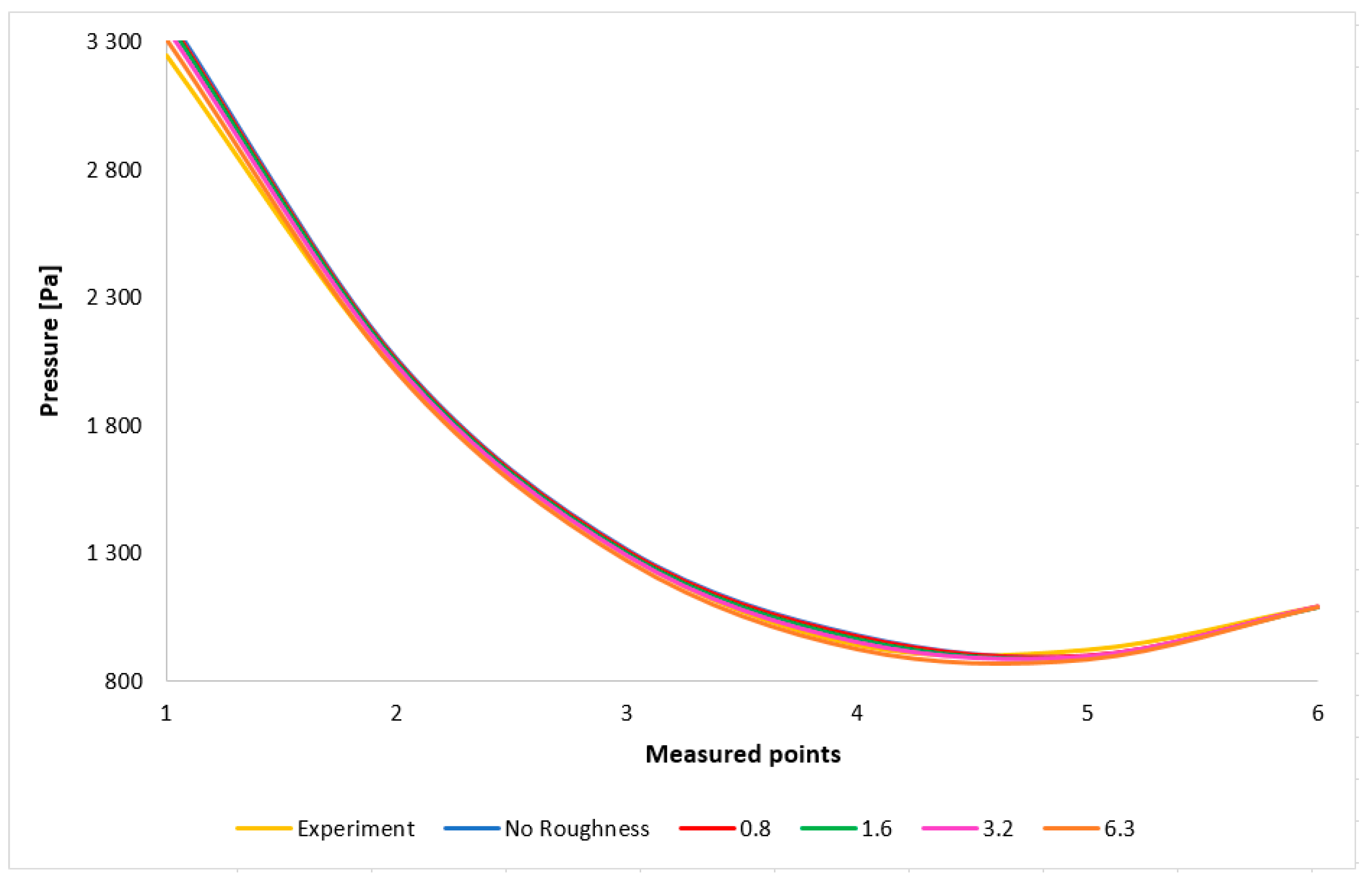
A comparison of the results reveals that the data acquired from the CFD analysis demonstrate a high level of precision relative to the experimental measurements. The correlation between the experimental and CFD simulation results is illustrated in Figure 9.
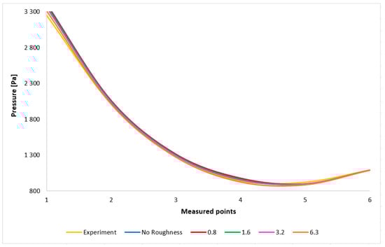
Figure 9.
Comparison of the results obtained using Ansys Fluent and experimental measurements.
The results indicate that the No Roughness variant exhibited the largest error. Roughness has a discernible impact on the accuracy of CFD simulations, although the error is negligible. The second-largest error was observed in the 0.8 roughness variant. The nozzle was manufactured with a roughness of 1.6, which resulted in a CFD simulation error of less than 2%. Surprisingly, variants with higher roughness values (3.2 and 6.3) exhibited even smaller errors, with the 3.2 variant being the most accurate. This effect is likely due to the presence of small pressure tap holes, spirally distributed on the nozzle wall (Figure 2), and the possibility that the nozzle was manufactured closer to the 3.2 roughness value within the manufacturing tolerances.
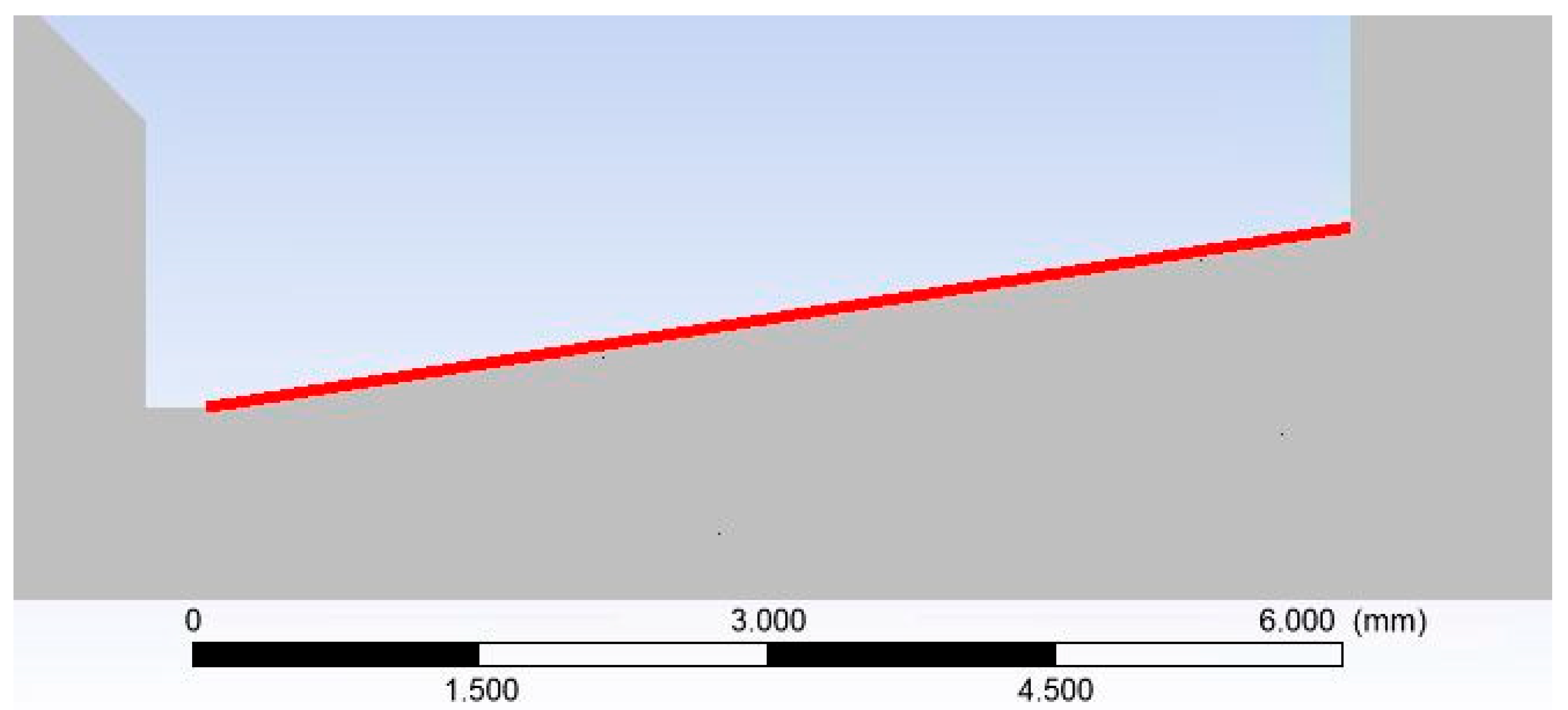
In the subsequent analysis, the flow field within the CFD simulations was examined. Initially, the wall pressure and temperature distributions on the nozzle surface were analyzed. This region corresponds to the location where pressure measurements were acquired experimentally. Figure 10 illustrates the specific path along which these quantities were extracted.

Figure 10.
Examined nozzle surface (red line—path).
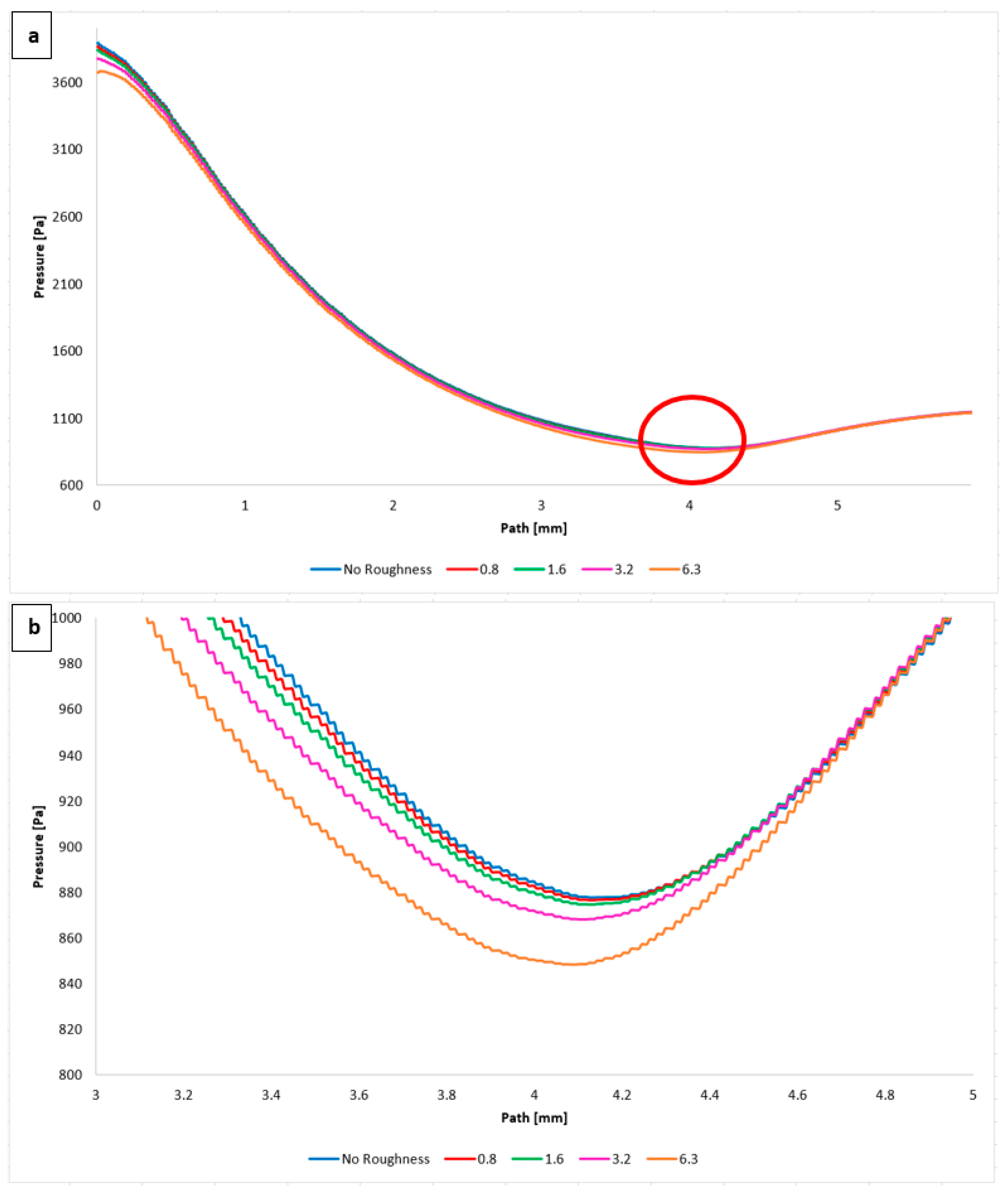
Figure 11a presents the static pressure distribution. A discontinuity caused by an oblique shock wave is evident at approximately 4 mm. The discontinuity region, circled in red, is magnified in Figure 11b using an adjusted scale to highlight the differences between the variants. Figure 11b clearly shows that the pressure drop increases with increasing surface roughness. The difference between the No Roughness variant and the 6.3 variant is as much as 30 Pa. Given that the variants of 3.2 and 6.3 exhibit the smallest errors compared to the experimental measurements, this is a significant finding for future research in ESEM development.
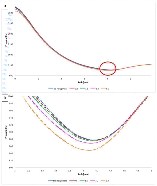
Figure 11.
Pressure distribution on the nozzle wall (path) (a) with zoomed red circle area with adjusted scale (b).
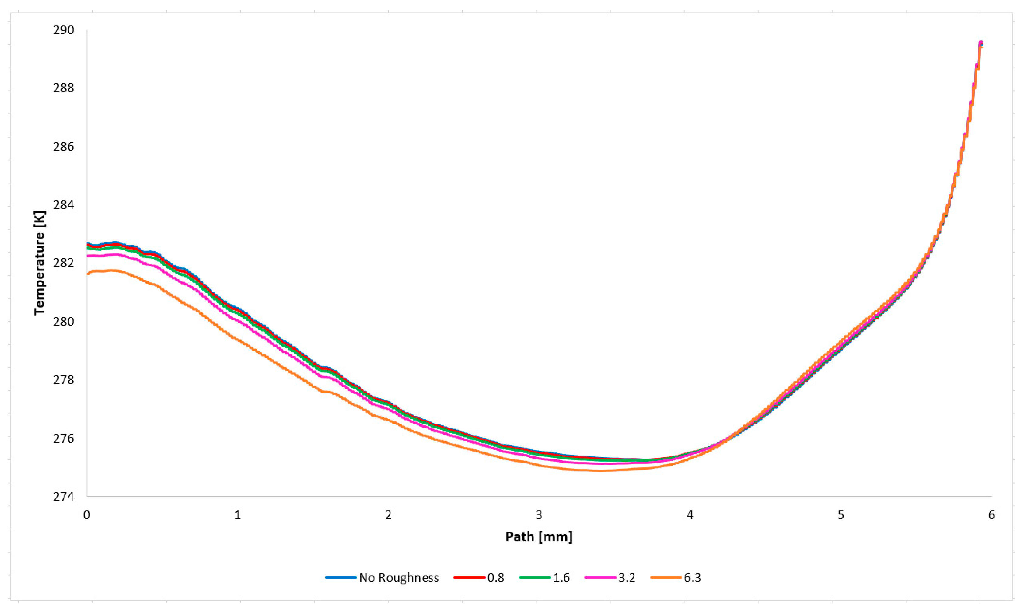
Future research will involve temperature measurements on the nozzle wall. The temperature distribution along the nozzle wall, illustrated in Figure 12, demonstrates the anticipated correlation with the static pressure distribution, thereby providing a suitable basis for validation.

Figure 12.
Temperature distribution on the nozzle wall (path).
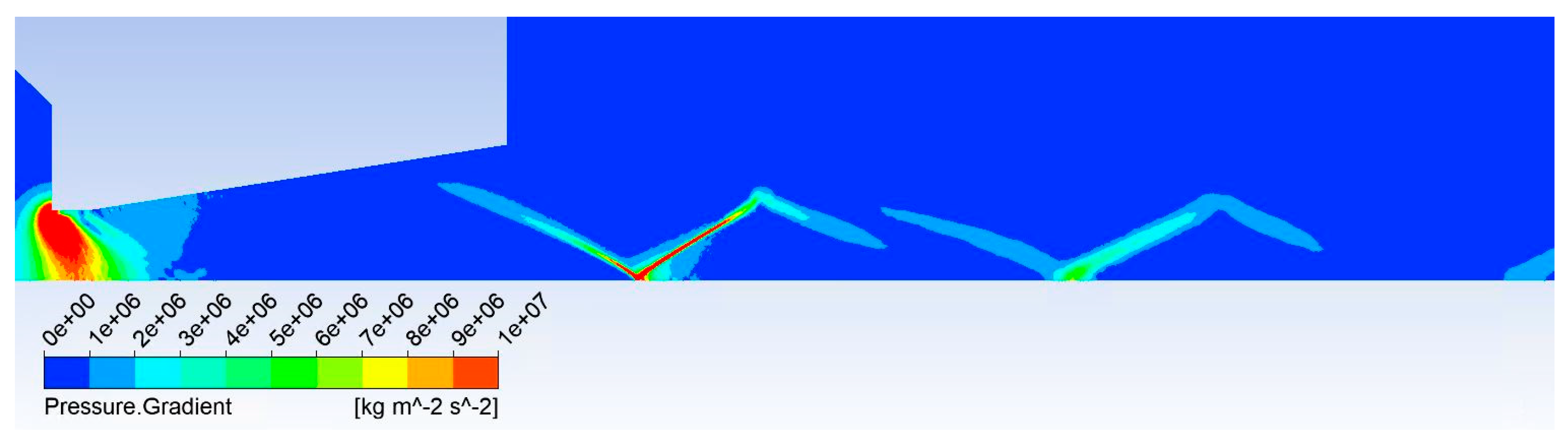
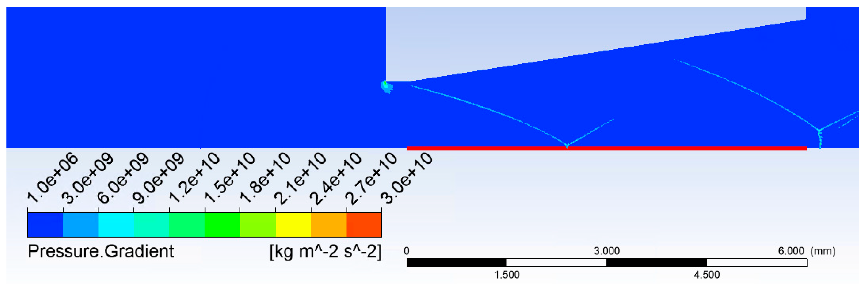
The aforementioned oblique shock wave is visualized in Figure 13, which presents the pressure gradient distribution. This shock wave influences the boundary layer (Figure 14a). A magnified view of this region with an adjusted scale is provided in Figure 14b to highlight these pressure gradients.
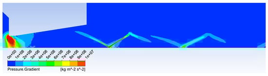
Figure 13.
Pressure gradient layout in the nozzle.
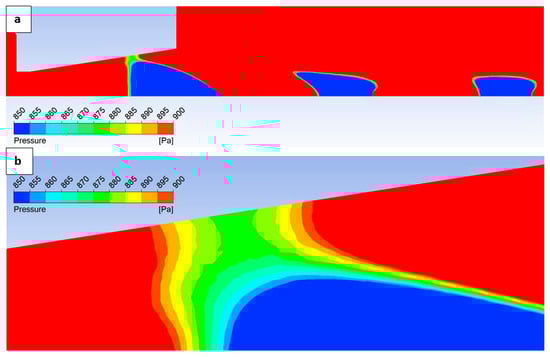
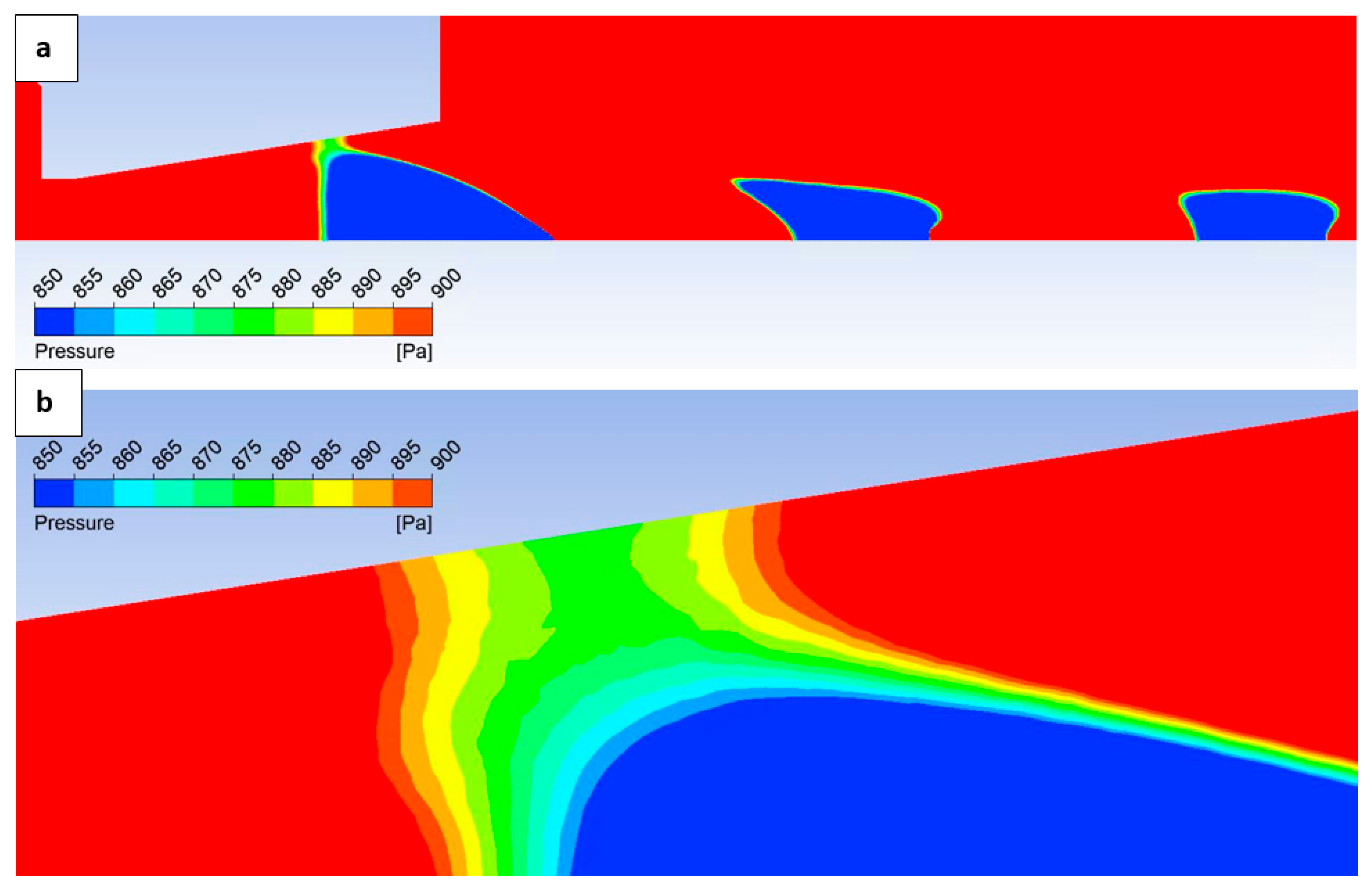
Figure 14.
Pressure layout in the nozzle (a) with the zoomed region with adjusted scale (b).
The analysis reveals a clear interaction between the oblique shock wave and the boundary layer in the studied variant. This interaction influences subsequent axial flow analysis. However, this influence is less pronounced under atmospheric pressure conditions, as will be further discussed in the flow analysis.
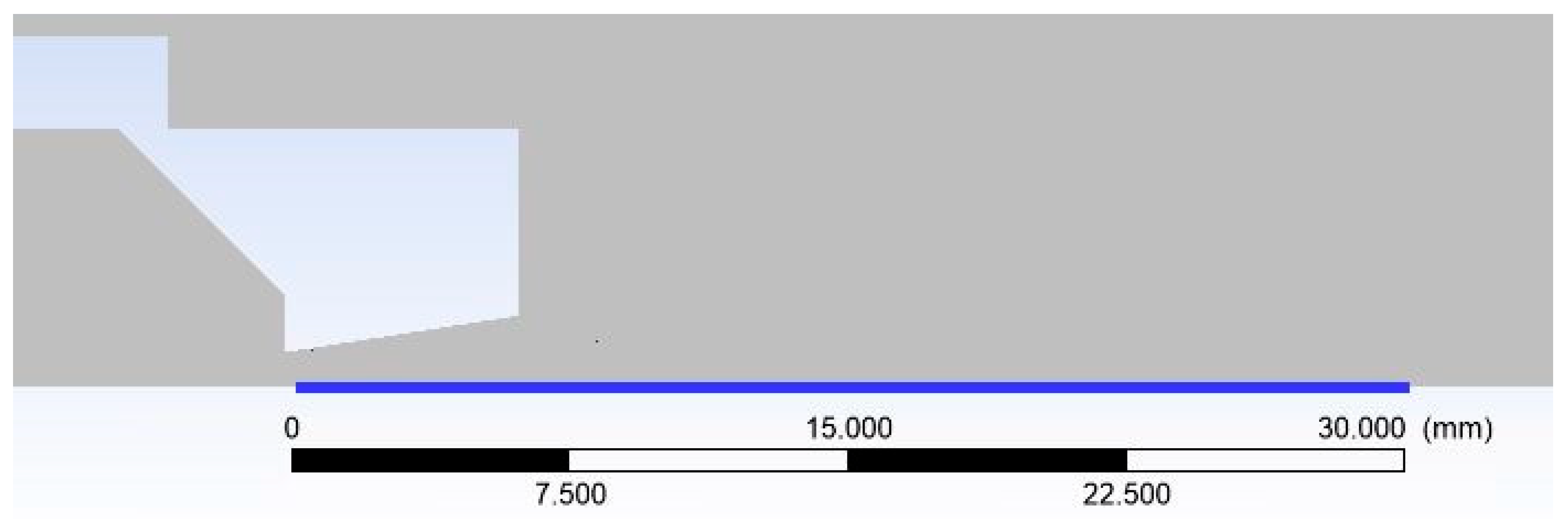
The subsequent analysis presents the axial flow profile within the nozzle, which may be influenced by boundary layer behavior. Figure 15 illustrates the axial flow path along which selected state variables are plotted.
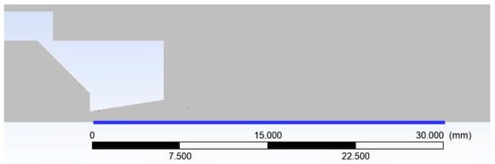
Figure 15.
Examined axial flow path (blue line—flow axis).
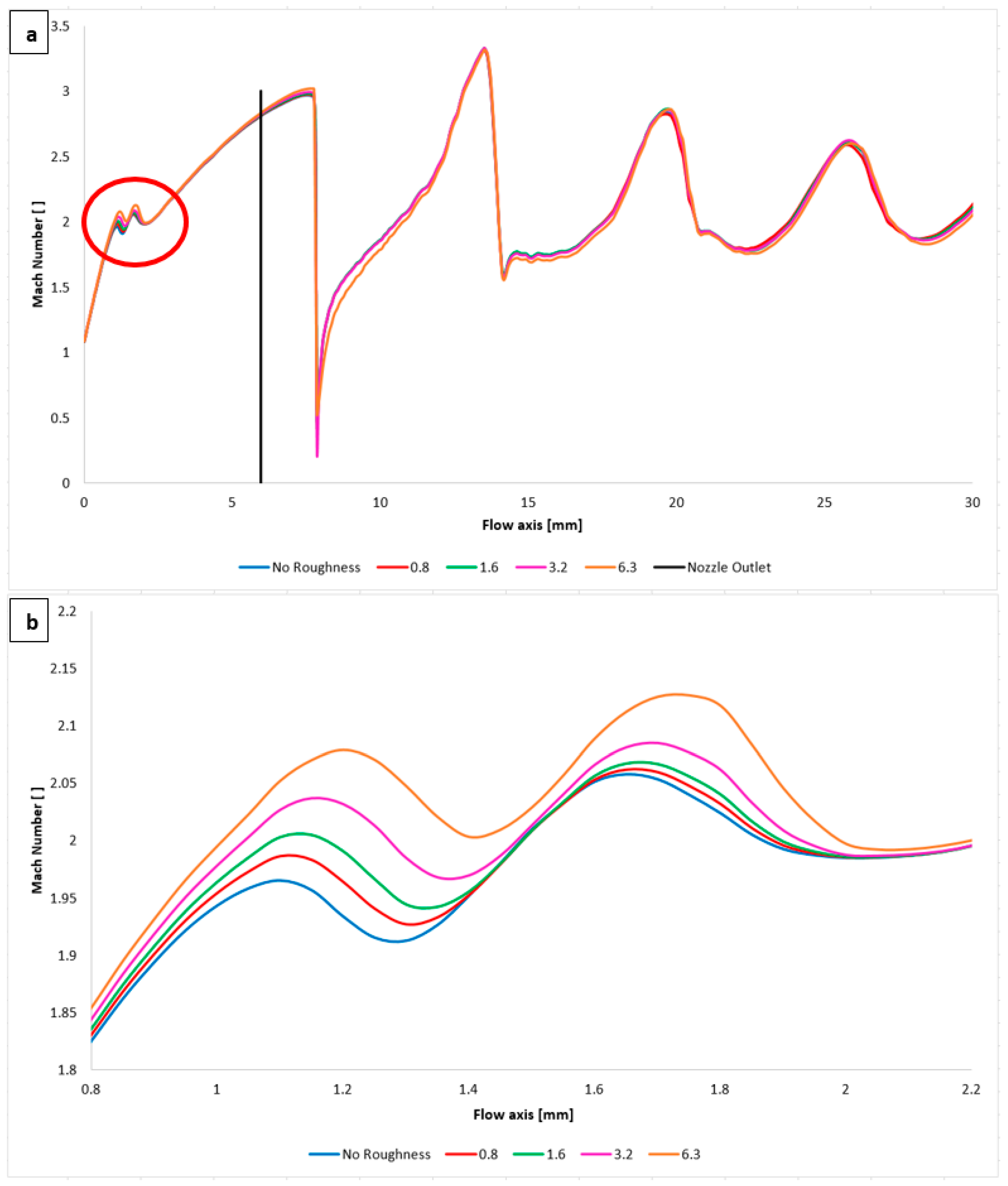
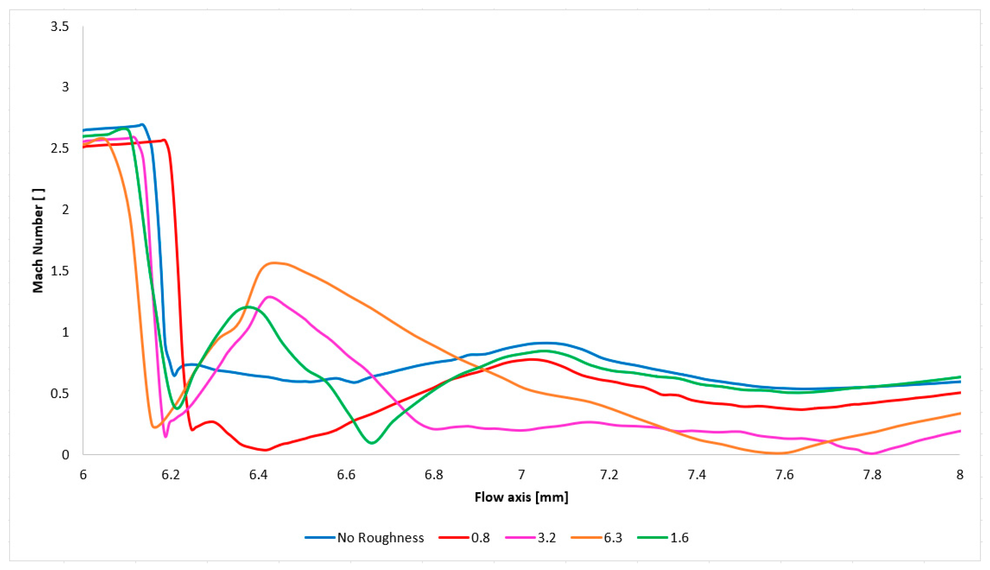
Figure 16a presents the Mach number distribution, highlighting the regions influenced by shock waves that interact with the boundary layer as previously discussed. The area affected by these shock waves is circled in red in Figure 16a. Figure 16b provides a magnified view of this region to reveal the variations in the nozzle flow caused by the oblique shock waves. The results indicate that a higher surface roughness leads to a higher flow velocity downstream of the aperture, until the velocity decreases due to the formation of the oblique shock wave.
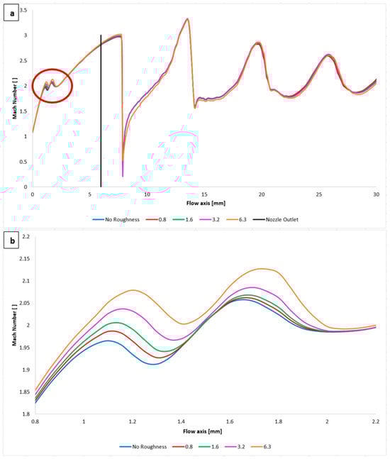
Figure 16.
Mach number distribution in the flow axis (a) with zoomed red circle area with adjusted scale (b).
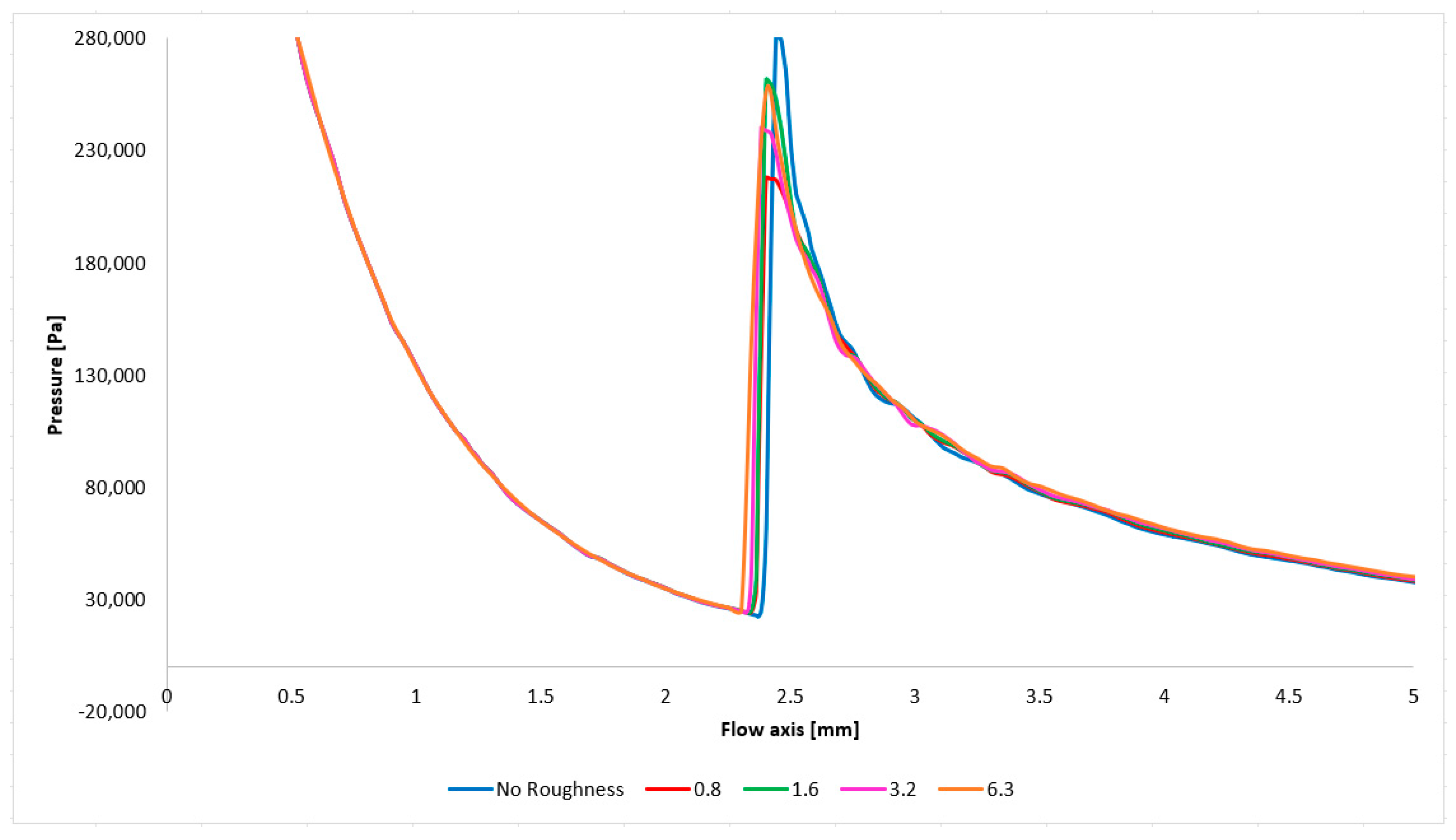
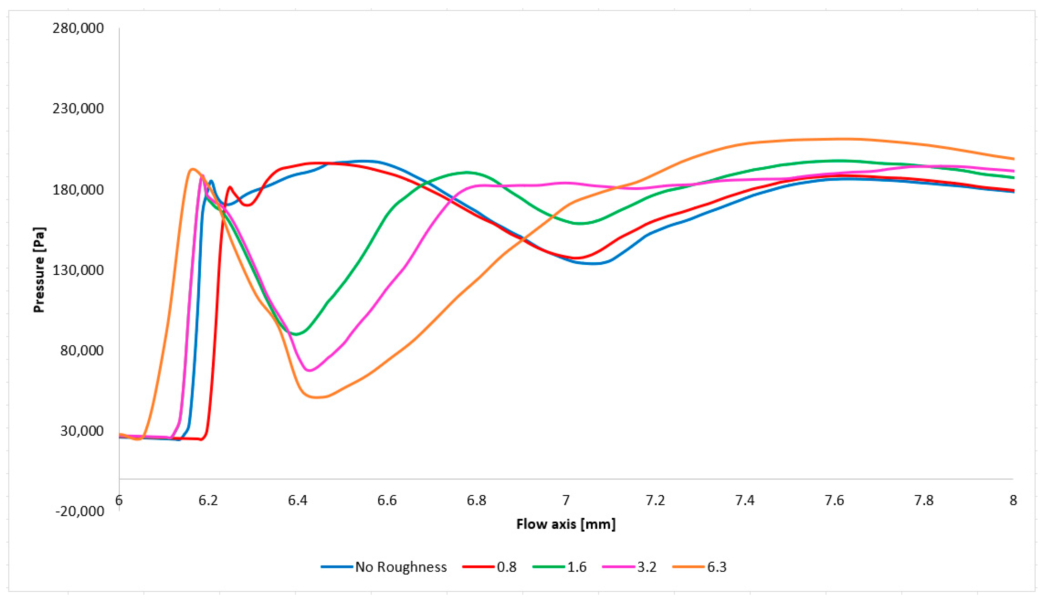
The Mach number distribution indicates that this phenomenon results in a more pronounced pressure drop ahead of the oblique shock wave (Figure 17a with a magnified red circled region in Figure 17b). This finding may influence the electron beam dispersion as it passes through the differentially pumped chamber, particularly if a lower average static pressure can be achieved along the given path.
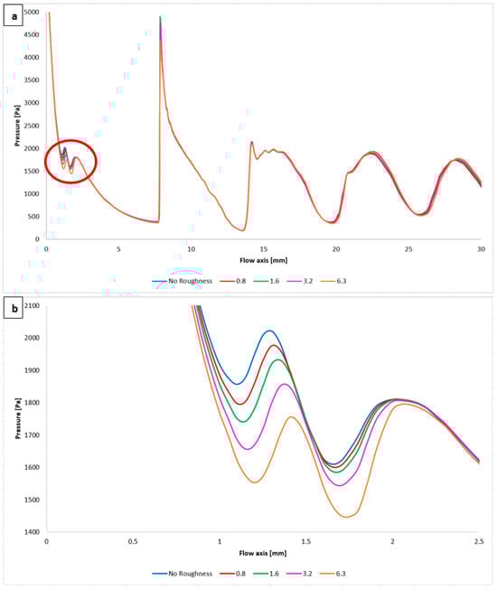
Figure 17.
Pressure distribution in the flow axis (a) with zoomed red circle area with adjusted scale (b).
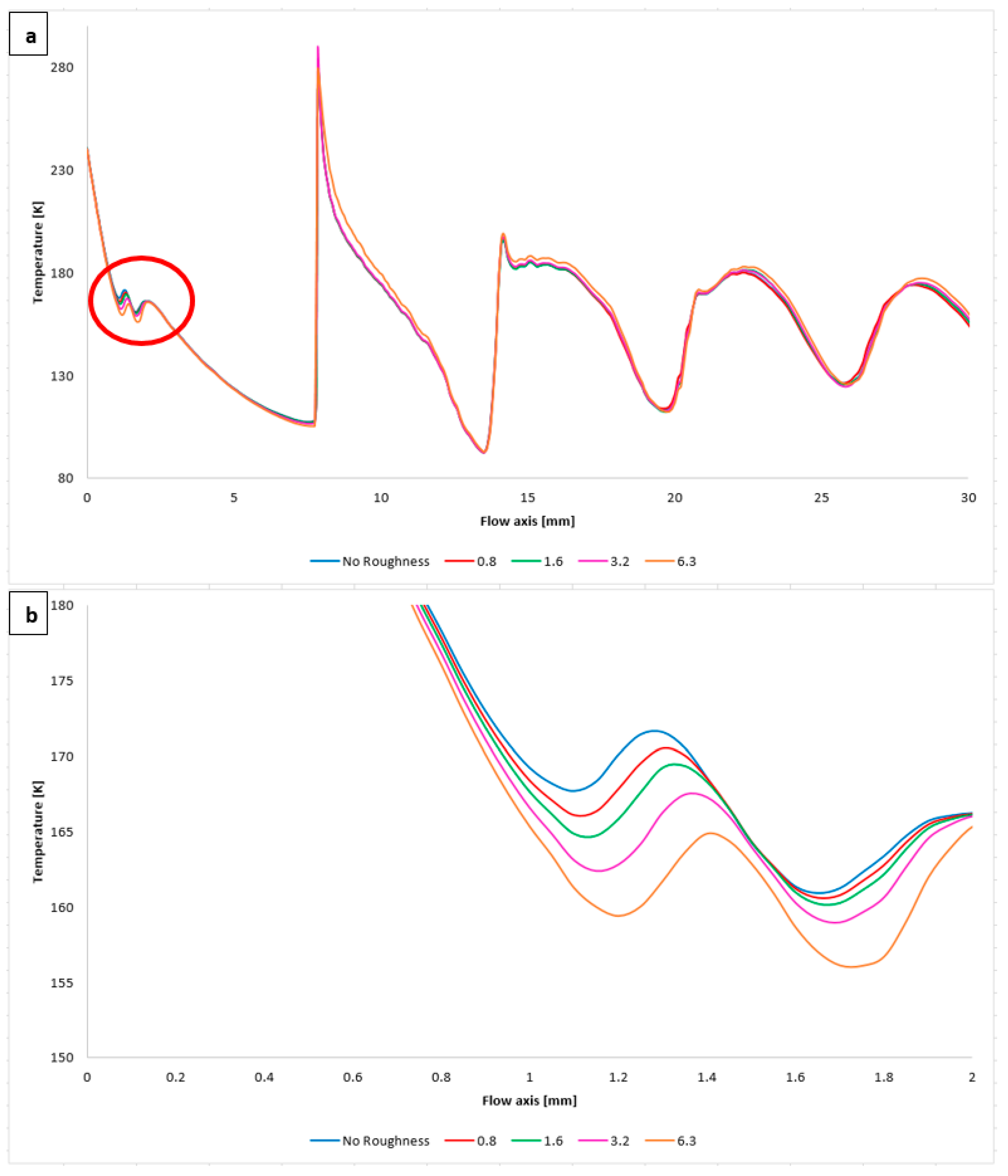
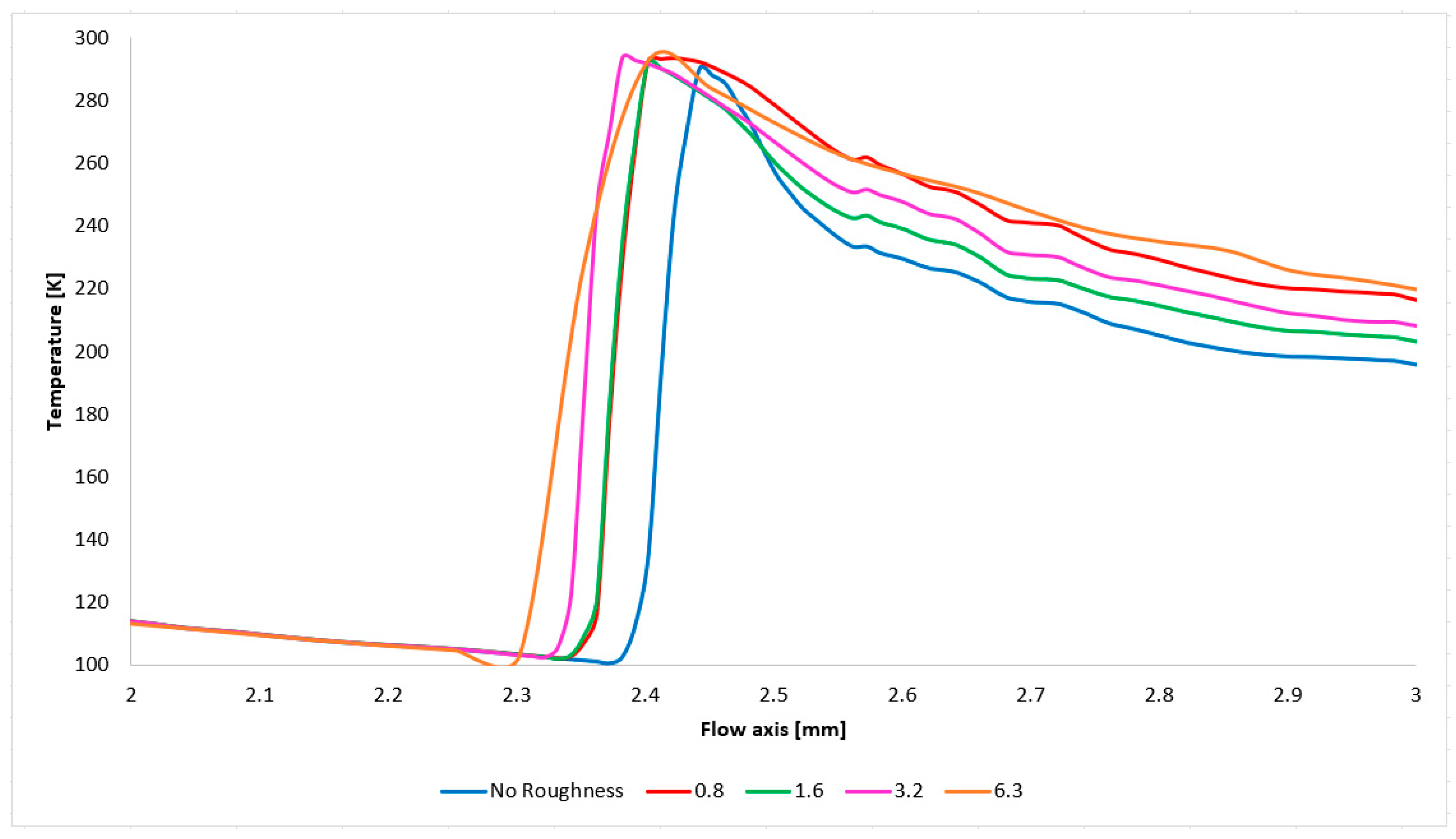
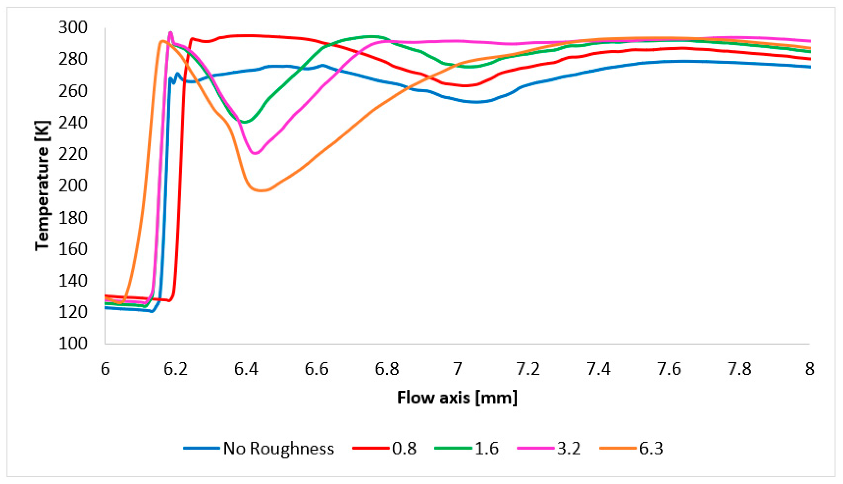
To provide a more comprehensive understanding of the flow characteristics, temperature profiles are included, which correlate with the Mach number and static pressure distributions along the given flow axis (Figure 18a with a magnified red circled region in Figure 18b). The temperature in regions of high Mach numbers decreases to cryogenic levels. Differences between the variants reach up to 10 °C.

Figure 18.
Temperature distribution in the flow axis (a) with zoomed red circle area with adjusted scale (b).
4.2. CFD Analysis Result for Atmospheric Variant
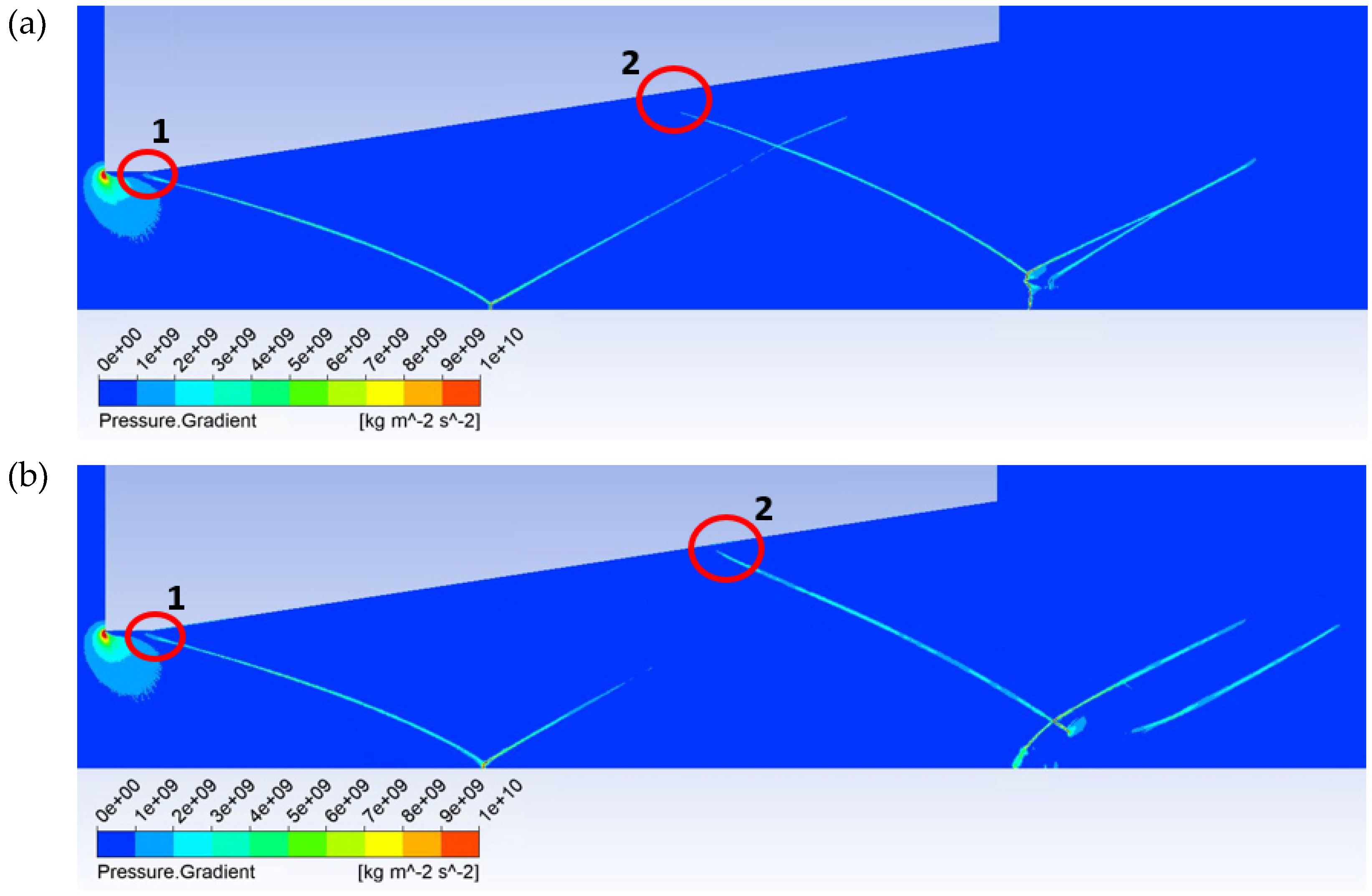
In the first step, similar to the previous subchapter, an analysis of the pressure distribution on the nozzle wall along the path shown in Figure 10 was performed. Here, in the ATM variant, a much more pronounced effect of roughness on the pressure profile and distribution on the nozzle wall is evident. This causes the effect described for the boundary layer in the methodology chapter. Additionally, it is apparent that, in contrast to the low-pressure case where only one wider oblique shock wave formed in the nozzle, in the ATM variant, two very pronounced and thin oblique shock waves form in the nozzle which in turn impact two locations in the boundary layer (Figure 19: red circles 1 and 2).
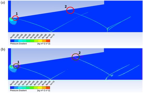
Figure 19.
Pressure gradient layout in the nozzle for No Roughness variant (a) and 6.3 variant (b).
Figure 19 presents the pressure gradient distribution for two variants: the No Roughness variant (Figure 19a) and the 6.3 variant (Figure 19b). It is evident that the 6.3 variant exhibits a more substantial intrusion of the pressure gradient into the boundary layer.
Three distinct flow regimes may manifest during the outflow from a nozzle. Firstly, a computational state exists where the ambient pressure, into which the gas discharges, is equivalent to the nozzle outlet pressure. In this case, the gas outflow exhibits a uniform characteristic. Secondly, a regime of reduced backpressure occurs when the ambient pressure is lower than the nozzle output pressure. This results in the initial formation of expansion waves at the nozzle aperture, which subsequently transition into compression waves after a certain distance. Oblique shock waves arise between these waves. Thirdly, a regime of elevated backpressure is observed when the ambient pressure exceeds the nozzle exit pressure. In this case, compression waves are initially formed at the nozzle aperture, which then transform into expansion waves after a certain distance. Oblique shock waves also develop between these waves [20].
In this scenario, the nozzle operates in an underexpanded state, characterized by elevated backpressure conditions. This results in the formation of compression waves downstream of the nozzle exit, interspersed with oblique shock waves exhibiting a needle-shaped morphology.
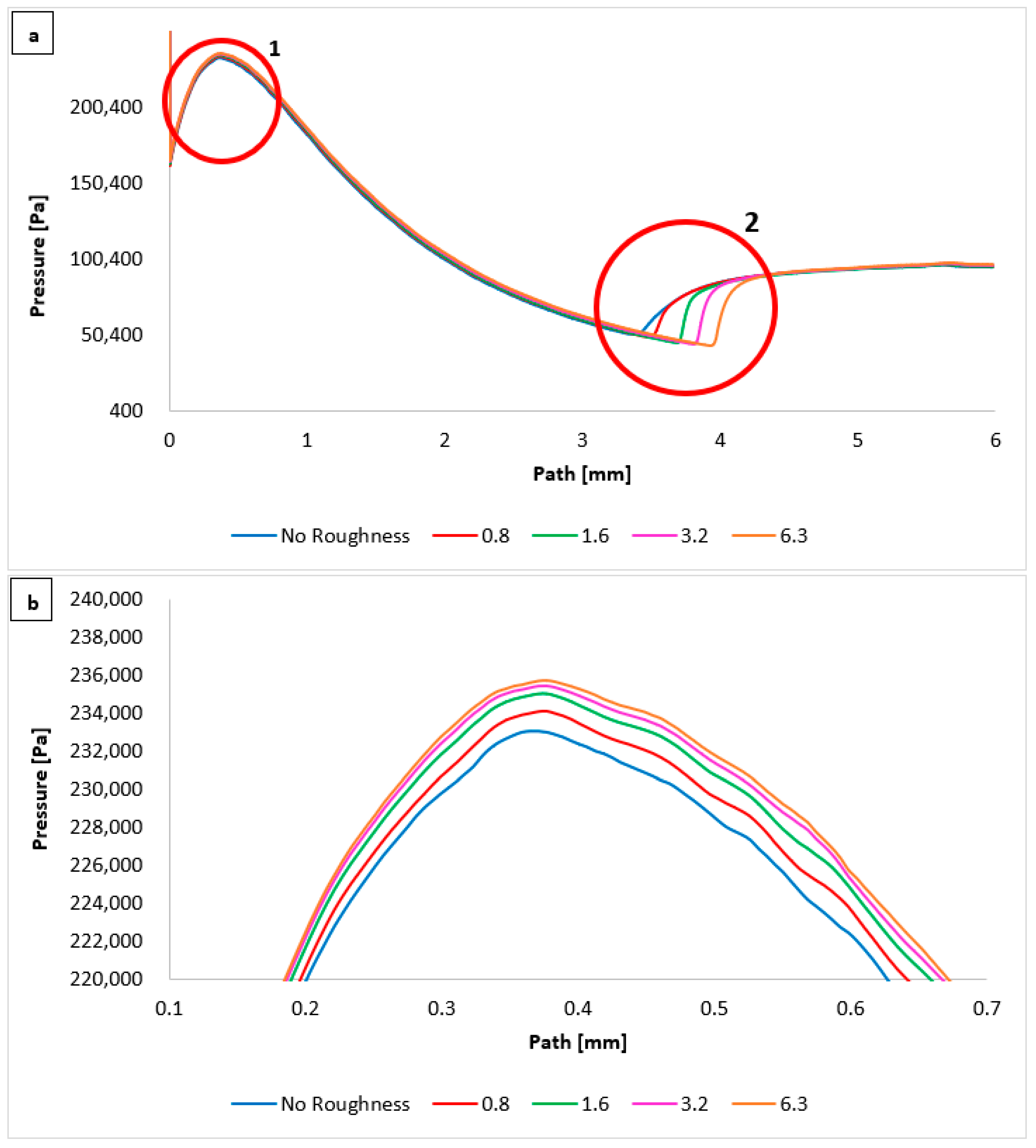
The static pressure distribution along the nozzle surface, as illustrated in Figure 20, demonstrates a distinct profile compared to the low-pressure case. The interactions of the oblique shock wave with the boundary layer at both identified locations are evident. In region 1, depicted in Figure 20a, a pressure increase behind the first oblique shock wave is evident. The results indicate that the roughness setting influences the resulting profile. Figure 20b presents an adjusted scale to highlight the difference in pressure magnitude at region 1. It is apparent that with increasing roughness values, the pressure behind the oblique shock wave also increases. However, as the surface roughness value increases further, this effect gradually diminishes.

Figure 20.
Pressure distribution on the nozzle wall (path) (a) with zoomed red circle 1 area with adjusted scale (b).
In the subsequent analysis of the results, profiles of state variables are presented along the flow direction. It is evident that the flow characteristics described by these profiles are influenced by changes in the shock wave caused by varying roughness values. These roughness-induced changes, as noted earlier, have a profound impact on the boundary layer development.
The Mach number distribution, restricted to the shock wave influence region at point 1 within the boundary layer, is depicted in Figure 21. For better visualization, Figure 22 highlights the flow axis with a scale. This figure clearly shows that the oblique shock wave, which interacts with the boundary layer at point 1, terminates on the flow axis at approximately a distance of 2.3, transitioning into a short normal shock wave. This phenomenon is a consequence of the condition of the underexpanded nozzle.
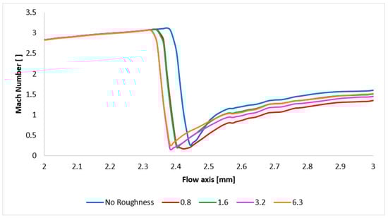
Figure 21.
Mach number distribution in the flow axis of the region 1.

Figure 22.
Pressure gradient layout in the nozzle with the scale.
The results demonstrate a different dependency compared to low-pressure conditions. This is attributed to the lower intensity of the oblique shock wave at low pressures. This oblique wave interacts with and influences the boundary layer to a much lesser extent than the oblique shock wave under atmospheric conditions. Consequently, at atmospheric pressure, the flow velocity for variants 0.8 and 1.6 decreases less compared to the No Roughness variant. For variants with higher roughness values (3.2 and 6.3), the velocity decreases to a lower value than that of the No Roughness variant.
This decrease in velocity influences the pressure distribution along the flow axis. This distribution is shown in Figure 23 and is directly correlated with the velocity profile. A greater decrease in velocity results in a larger increase in static pressure across the shock wave. This affects the dispersion of the passing electron beam, which requires the lowest possible pressure along its path.
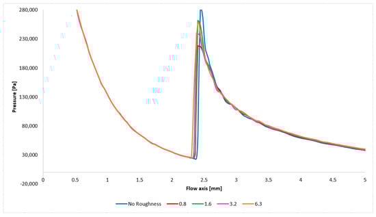
Figure 23.
Pressure distribution in the flow axis of region 1.
The temperature distribution presented in Figure 24 provides additional insights into the nature of the flow passing through the shock wave.
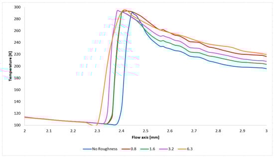
Figure 24.
Temperature distribution in the flow axis of region 1.
In region 2 (Figure 20a), it is evident that the smooth variant exhibits a smaller pressure gradient at the discontinuity caused by the oblique shock wave interacting with the boundary layer compared to the variant with the highest roughness value (variant 6.3) (Figure 25).

Figure 25.
Pressure distribution on the nozzle wall (path) with adjusted scale of region 2.
This effect is caused by a significantly more pronounced oblique shock wave compared to the 1158 Pa variant. Consequently, the influence of surface roughness on the differences in this oblique shock wave interacting with the boundary layer under atmospheric pressure becomes more evident. This interaction of the oblique shock wave induces a small boundary layer separation and the formation of lambda shocks, which are captured in the simulations using the SST-omega turbulence model with a blending function in the manner presented. This phenomenon is illustrated in Figure 26 for variant 6.3. The other variants, due to their lesser interaction with the oblique shock wave, exhibit a broader distribution of this effect.
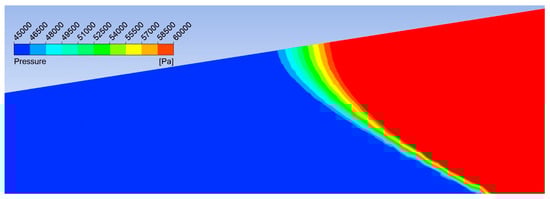
Figure 26.
Pressure layout in the nozzle for 6.3 variant of region 2.
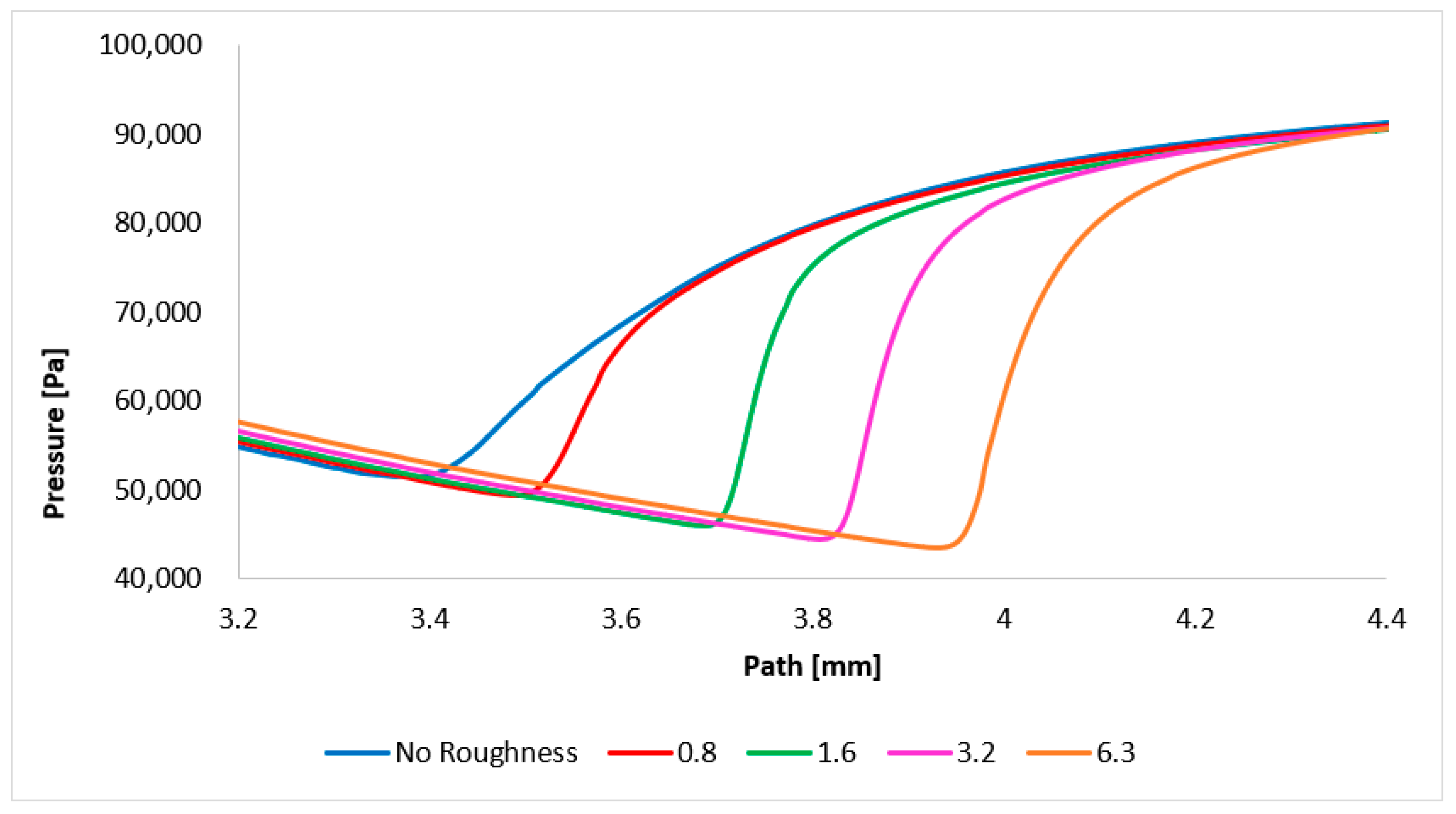
This alteration in the boundary layer can influence the axial flow. Figure 27 reveals that the pressure distribution is primarily affected by the shift in the normal shock wave along the flow axis. Relative to the No Roughness variant, the variant with a very fine roughness initially exhibits a slight downstream shift of the shock wave from the aperture. Subsequently, with increasing roughness, the shock wave moves closer to the aperture. However, this shift is also significantly influenced by the position of the first shock wave. A distinct flow behavior is observed downstream of the second shock wave for both the No Roughness and the very fine roughness (variant 0.8) cases, characterized by oscillations and subsequent pressure increases. This is attributed to the minimal decrease in Mach number at the first shock wave for the No Roughness and 0.8 variants.
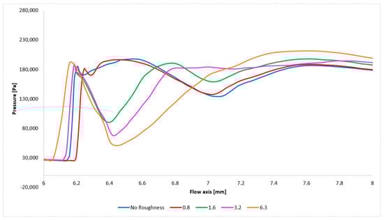
Figure 27.
Pressure distribution in the flow axis of region 2.
This aligns with the Mach number distribution presented in Figure 28, where the No Roughness and 0.8 variants do not exhibit a subsequent increase in velocity above 1 Mach. This is because at the end of the oblique shock wave, a short normal shock wave crossing the flow axis does not form, but only oblique shock waves intersect. Conversely, for variants with higher roughness (1.6, 3.2, and 6.3), the velocity increases again to supersonic speeds. Consequently, a short normal shock wave forms at the intersection of the oblique shock waves. It is evident that roughness influences the flow characteristics by transforming nozzles with dimensions close to the design regime into a type of underexpanded nozzle.
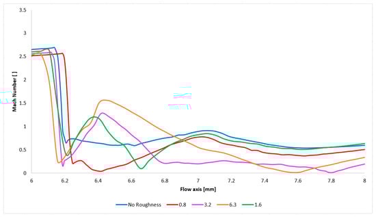
Figure 28.
Mach number distribution in the flow axis of region 2.
The temperature distribution depicted in Figure 29 further corroborates the flow description and is consistent with the Mach number and static pressure profiles.
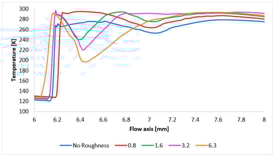
Figure 29.
Temperature distribution in the flow axis of region 2.
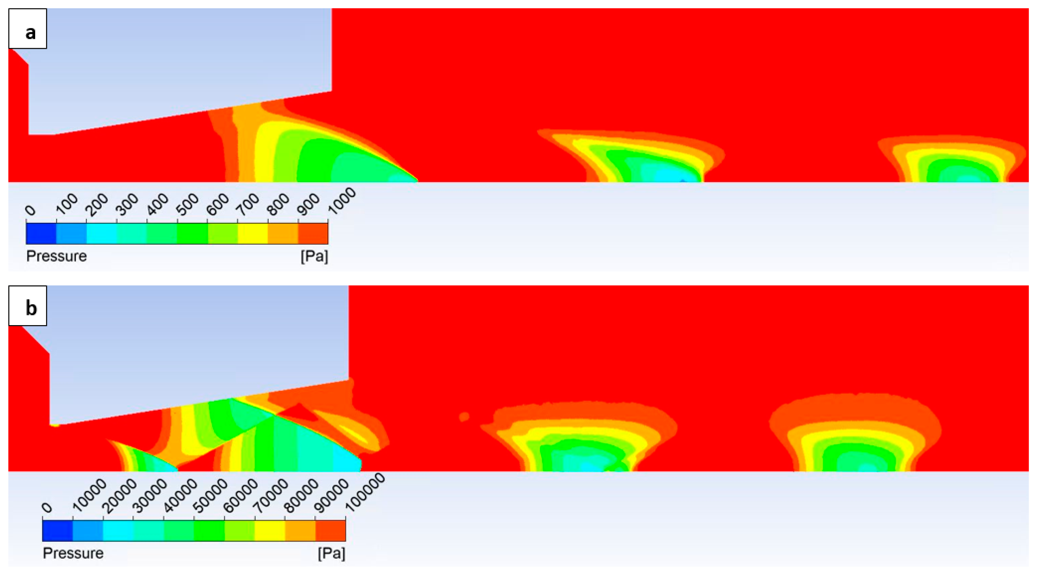
To provide a comprehensive comparison of the flow behavior within the nozzle under both atmospheric and low-pressure conditions, within the framework of continuum mechanics, a summary is presented in the following figure. Figure 30a illustrates the pressure distribution for the 1158 Pa variant, while Figure 30b shows the distribution for the ATM variant.
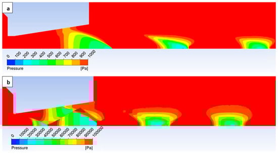
Figure 30.
Pressure layout in the nozzle for 1158 Pa variant (a) and ATM variant (b).
The relative magnitudes of inertial and viscous forces in low-pressure environments differ substantially from those observed under atmospheric conditions, as previously discussed. In low-pressure environments, viscous forces dominate. Consequently, inertial forces are insufficient to generate a pair of oblique shock waves, as observed in the atmospheric pressure variant. The oblique shock wave in the low-pressure variant interacts with the boundary layer to a much lesser extent (Figure 30a) compared to the atmospheric variant (Figure 30b). This is illustrated by a figure with a scale adjusted to represent approximately similar flow characteristics.
5. Conclusions
A combined experimental and computational fluid dynamics (CFD) analysis to investigate the influence of surface roughness on supersonic flow and the characteristics of shock wave distribution within a nozzle operating under both atmospheric and low-pressure conditions is presented in this paper.
In the initial phase, repeated experimental measurements of static pressure were conducted on the nozzle surface, from which the standard error of the mean (SEM) was evaluated for a pressure variant of 1158 Pa. The resulting SEM values for all measured points did not exceed 1.5 Pa.
In the second phase of the analysis, the experimental results of the measured static pressure were compared with those obtained from CFD simulations for varying surface roughness values. The comparison between experimental and CFD results demonstrated a relative error not exceeding 3%.
Subsequently, CFD analyses were performed for the atmospheric pressure variant across the same range of surface roughness values, and these results were compared with the results obtained from the 1158 Pa pressure variant.
It has been demonstrated that in low-pressure regimes, where viscous forces dominate, only a single oblique shock wave forms within the nozzle. This wave is characterized by a more pronounced profile and reduced penetration into the boundary layer. Conversely, atmospheric conditions, with their more significant inertial forces, generate two intense oblique shock waves that exhibit substantial interaction with the boundary layer. Consequently, the influence of surface roughness is more pronounced under atmospheric conditions. These findings will be applied to further research in the field of differentially pumped chambers.
Author Contributions
Conceptualization, J.M. and P.Š.; methodology, J.M. and P.Š.; software, J.M. and P.Š.; validation, J.M., J.Š., M.V. and P.B.; formal analysis, J.M., P.Š. and T.B.; investigation, J.M., P.Š., J.Š. and P.B.; resources, T.B., J.T. and R.B.; data curation, J.M., R.B. and P.Š.; writing—original draft preparation, J.M. and P.Š.; writing—review and editing, P.Š., T.B. and J.T.; visualization, P.Š. and R.B.; supervision, J.M., J.Š. and T.B.; project administration, M.V. and J.Š.; funding acquisition, J.Š., J.T. and P.B. All authors have read and agreed to the published version of the manuscript.
Funding
This work was supported by the Ministry of Defence of the Czech Republic project No. DZRO K-109, by the specific graduate research of the Brno University of Technology No. FEKT-S-23-8286, and by the IG Agency of Mendel University in Brno, Faculty of AgriSciences, project No. IGA24-AF-IP-046.
Institutional Review Board Statement
Not applicable.
Informed Consent Statement
Not applicable.
Data Availability Statement
The data presented in this study are available on request from the corresponding author.
Conflicts of Interest
The authors declare no conflicts of interest.
Abbreviations
The following abbreviations are used in this manuscript:
| ESEM | Environmental Scanning Electron Microscope; |
| CFD | Computational fluid dynamics; |
| AUSM | Advection Upstream Splitting Method; |
| FSO | Full-Scale Output; |
| BFSL | Best Fit Straight Line |
References
- Vetráková, Ľ.; Neděla, V.; Runštuk, J.; Heger, D. The morphology of ice and liquid brine in an environmental scanning electron microscope: A study of the freezing methods. Cryosphere 2019, 13, 2385–2405. [Google Scholar] [CrossRef]
- Đorđević, B.; Neděla, V.; Tihlaříková, E.; Trojan, V.; Havel, L. Effects of copper and arsenic stress on the development of Norway spruce somatic embryos and their visualization with the environmental scanning electron microscope. New Biotechnol. 2019, 48, 35–43. [Google Scholar] [CrossRef] [PubMed]
- Neděla, V.; Hřib, J.; Vooková, B. Imaging of early conifer embryogenic tissues with the environmental scanning electron microscope. Biol. Plant. 2012, 56, 595–598. [Google Scholar] [CrossRef]
- Bezrukovs, V.; Bezrukovs, V.; Konuhova, M.; Bezrukovs, D.; Kaldre, I.; Popov, A.I. Numerical Simulations of Thermodynamic Processes in the Chamber of a Liquid Piston Compressor for Hydrogen Applications. Technologies 2024, 12, 266. [Google Scholar] [CrossRef]
- Zhu, Y.; Fukuda, T.; Yabuki, N. Integrating Animated Computational Fluid Dynamics into Mixed Reality for Building-Renovation Design. Technologies 2020, 8, 4. [Google Scholar] [CrossRef]
- Kurkin, E.; Minaev, E.; Sedelnikov, A.; Pioquinto, J.G.Q.; Chertykovtseva, V.; Gavrilov, A. Computer Vision Technology for Short Fiber Segmentation and Measurement in Scanning Electron Microscopy Images. Technologies 2024, 12, 249. [Google Scholar] [CrossRef]
- Chelopo, D.; Gupta, K. A Comparative Evaluation of Conveyor Belt Disc Brakes and Drum Brakes: Integrating Structural Topology Optimization and Weight Reduction. Technologies 2024, 12, 136. [Google Scholar] [CrossRef]
- Stelate, A.; Tihlaříková, E.; Schwarzerová, K.; Neděla, V.; Petrášek, J. Correlative Light-Environmental Scanning Electron Microscopy of Plasma Membrane Efflux Carriers of Plant Hormone Auxin. Biomolecules 2021, 11, 1407. [Google Scholar] [CrossRef]
- Neděla, V. Methods for Additive Hydration Allowing Observation of Fully Hydrated State of Wet Samples in Environmental SEM. Microsc. Res. Tech. 2007, 70, 95–100, ISSN 1059-910X. E-ISSN 1097-0029. [Google Scholar] [CrossRef]
- Vlašínová, H.; Neděla, V.; Dordevic, B.; Havel, J. Bottlenecks in bog pine multiplication by somatic embryogenesis and their visualization with the environmental scanning electron microscope. Protoplasma 2017, 254, 1487–1497, ISSN 0033-183X. E-ISSN 1615-6102. [Google Scholar] [CrossRef]
- Danilatos, G.D. Velocity and ejector-jet assisted differential pumping: Novel design stages for environmental SEM. Micron 2012, 43, 600–611. [Google Scholar] [CrossRef]
- Danilatos, G.D. Figure of merit for environmental SEM and its implications. J. Microsc. 2011, 244, 159–169. [Google Scholar] [CrossRef] [PubMed]
- Danilatos, G.D. Optimum beam transfer in the environmental scanning electron microscope. J. Microsc. 2009, 234, 26–37. [Google Scholar] [CrossRef] [PubMed]
- Danilatos, G.D.; Rattenberger, J.; Dracopoulos, V. Beam transfer characteristics of a commercial environmental SEM and a low vacuum SEM. J. Microsc. 2011, 242, 166–180. [Google Scholar] [CrossRef]
- Hlavatá, P.; Maxa, J.; Vyroubal, P. Analysis of Pitot Tube Static Probe Angle in the Experimental Chamber Conditions. ECS Trans. 2018, 87, 369–375. [Google Scholar] [CrossRef]
- Maxa, J.; Šabacká, P.; Mazal, J.; Neděla, V.; Binar, T.; Bača, P.; Talár, J.; Bayer, R.; Čudek, P. The Impact of Nozzle Opening Thickness on Flow Characteristics and Primary Electron Beam Scattering in an Environmental Scanning Electron Microscope. Sensors 2024, 24, 2166. [Google Scholar] [CrossRef]
- Versteeg, H.K.; Malalasekera, W. An Introduction to Computational Fluid Dynamics; John Wiley & Sons: New York, NY, USA, 1995. [Google Scholar]
- Ferziger, J.H.; Perić, M. Computational Methods for Fluid Dynamics, 3rd ed.; Springer: Berlin/Heidelberg, Germany, 2002. [Google Scholar]
- Blazek, J. Computational Fluid Dynamics: Principles and Applications; Elsevier: Oxford, UK, 2001. [Google Scholar]
- Lipej, A.; Muhič, S.; Mitruševski, D. Wall Roughness Influence on The Efficiency Characteristics of Centrifugal Pump. J. Mech. Eng. 2017, 63, 529–536. [Google Scholar] [CrossRef]
- Moran, M.J.; Shapiro, H.N. Fundamentals of Engineering Thermodynamics, 3rd ed.; John Wiley: New York, NY, USA, 1998. [Google Scholar]
- Dejč, M.J. Technická Dynamika Plynů; SNTL: Prague, Czech Republic, 1967. [Google Scholar]
- Nasuti, F.; Onofri, M. Shock structure in separated nozzle flows. Shock Waves 2008, 19, 229–237. [Google Scholar] [CrossRef]
- Daněk, M. Aerodynamika a Mechanika Letu; VVLŠ SNP: Košice, Slovak Republic, 1990. [Google Scholar]
- Maxa, J.; Neděla, V.; Šabacká, P.; Binar, T. Impact of Supersonic Flow in Scintillator Detector Apertures on the Resulting Pumping Effect of the Vacuum Chambers. Sensors 2023, 23, 4861. [Google Scholar] [CrossRef]
- Taylor, H.G.; Waldram, J.M. Improvements in the schlieren method. J. Sci. Instrum. 1933, 10, 378–389. [Google Scholar] [CrossRef]
- Richard, H.; Raffel, M. Principle and applications of the background oriented schlieren (BOS)method. Meas. Sci. Technol. 2001, 6, 1576–1585. [Google Scholar] [CrossRef]
- González-Durán, J.E.E.; Olivares-Ramírez, J.M.; Luján-Vega, M.A.; Soto-Osornio, J.E.; García-Guendulain, J.M.; Rodriguez-Resendiz, J. Experimental and Numerical Analysis of a Novel Cycloid-Type Rotor versus S-Type Rotor for Vertical-Axis Wind Turbine. Technologies 2024, 12, 54. [Google Scholar] [CrossRef]
- Drexler, P.; Čáp, M.; Fiala, P.; Steinbauer, M.; Kadlec, R.; Kaška, M.; Kočiš, L. A Sensor System for Detecting and Localizing Partial Discharges in Power Transformers with Improved Immunity to Interferences. Sensors 2019, 19, 923. [Google Scholar] [CrossRef] [PubMed]
- Pritchard, P.J. Introduction to Fluid Mechanics; John Wiley & Sons, Inc.: Hoboken, NJ, USA, 2011. [Google Scholar]
- Webster, J.G. Measurement, Instrumentation, and Sensors Handbook: Spatial, Mechanical, Thermal, and Radiation Measurement, 2nd ed.; Crc Pr: Boca Raton, FL, USA, 2014. [Google Scholar]
- Barth, T.; Jespersen, D. The design and application of upwind schemes on unstructured meshes. In Proceedings of the 27th Aerospace Sciences Meeting, Reno, NV, USA, 9–12 January 1989. [Google Scholar]
- Ansys Fluent Theory Guide. Available online: www.ansys.com (accessed on 21 October 2022).
- Beer, M.; Kudelas, D.; Rybár, R. A Numerical Analysis of the Thermal Energy Storage Based on Porous Gyroid Structure Filled with Sodium Acetate Trihydrate. Energies 2023, 16, 309. [Google Scholar] [CrossRef]
- Yang, Y.; Li, M.; Shu, S.; Xiao, A. High order schemes based on upwind schemes with modified coefficients. J. Comput. Appl. Math. 2006, 195, 242–251. [Google Scholar] [CrossRef]
- Vyroubal, P.; Maxa, J.; Kazda, T.; Vondrák, J. The Finite Element Method in Electrochemistry—Modelling of the Lithium-Ion Battery. ECS Trans. 2014, 48, 289–296. [Google Scholar] [CrossRef]
- Binar, T.; Svarc, J.; Vyroubal, P.; Kazda, T.; Rolc, S.; Dvorák, A.; Dostál, P. The Use of Numerical Simulation for the Evaluation of Special Transparent Glass Resistance. Eng. Fail. Anal. 2018, 91, 433–448. [Google Scholar] [CrossRef]
- Maxa, J.; Hlavatá, P.; Vyroubal, P. Using the Ideal and Real Gas Model for The Mathematical—Physics Analysis of the Experimental Chambre. ECS Trans. 2018, 87, 377–387. [Google Scholar] [CrossRef]
- Xiao, L.; Hao, X.; Lei, D.; Tiezhi, S. Flow structure and parameter evaluation of conical convergent–divergent nozzle supersonic jet flows. Phys. Fluids 2023, 35, 066109. [Google Scholar]
- Baehr, H.D.; Kabelac, S. Thermodynamik, 14th ed.; Springer: Berlin/Heidelberg, Germany, 2009. [Google Scholar]
- Liu, Q.; Feng, X.-B. Numerical Modelling of Microchannel Gas Flows in the Transition Flow Regime Using the Cascaded Lattice Boltzmann Method. Entropy 2020, 22, 41. [Google Scholar] [CrossRef]
- Yuan, T.-F.; Zhang, P.-J.-Y.; Liao, Z.-M.; Wan, Z.-H.; Liu, N.-S.; Lu, X.-Y. Effects of inflow Mach numbers on shock train dynamics and turbulence features in a backpressured supersonic channel flow. Phys. Fluids 2024, 36, 026126. [Google Scholar] [CrossRef]
- Dynamická Viskozita Plynů, E-Tabulky. Available online: https://uchi.vscht.cz/studium/tabulky/viskozita-plyny (accessed on 31 January 2025).
- The Engineering ToolBox, Nitrogen—Dynamic and Kinematic Viscosity vs.Temperature and Pressure. Available online: https://www.engineeringtoolbox.com/nitrogen-N2-dynamic-kinematic-viscosity-temperature-pressure-d_2067.html (accessed on 24 March 2025).
- Reimer, L. Scanning Elektron Microscopy: Physics of Image Formation and Microanalysis; Springer: Berlin/Heidelberg, Germany, 1985; ISBN 3540135308. [Google Scholar]
- Frank, L.; Král, J. Metody Analýzy Povrchů: Iontové, Sondové a Speciální Metody; Academia: Prague, Czech Republic, 2002; p. 489. ISBN 80-200-0594-3. [Google Scholar]
- Hermann, R. Supersonic Inlet Diffusers; Minneapolis-Honeywell Regulator Co., Aeronautical Division: Minneapolis, MN, USA, 1956. [Google Scholar]
- Afkhami, S.; Fouladi, N. Gas dynamics at starting and terminating phase of a supersonic exhaust diffuser with a conical nozzle. Phys. Fluids 2024, 36, 036123. [Google Scholar] [CrossRef]
- Pang, A.L.J.; Skote, M.; Lim, S.Y. Modelling high Re flow around a 2D cylindrical bluff body using the k–w (SST) turbulence model. Prog. CFD 2016, 16, 48–57. [Google Scholar] [CrossRef]


Disclaimer/Publisher’s Note: The statements, opinions and data contained in all publications are solely those of the individual author(s) and contributor(s) and not of MDPI and/or the editor(s). MDPI and/or the editor(s) disclaim responsibility for any injury to people or property resulting from any ideas, methods, instructions or products referred to in the content. |
© 2025 by the authors. Licensee MDPI, Basel, Switzerland. This article is an open access article distributed under the terms and conditions of the Creative Commons Attribution (CC BY) license (https://creativecommons.org/licenses/by/4.0/).