Foreign Direct Investment and Exports Stimulate Economic Growth? Evidence of Equilibrium Relationship in Peru

Abstract

The purpose of this research is to estimate the dynamic impacts of foreign direct investments (FDI) and exports on economic growth in Peru (1970–2020) using annual series. Starting with the theoretical Mundell–Fleming static model with assumptions, we find that the change in exports does not affect GDP, and the effect of FDI on GDP can be positive or negative depending on the comparison between the slopes of the IS and LM curves. The variables are foreign direct investment net flow (% of GDP), exports of goods and services (% of GDP), and GDP growth rate (%). FDI and exports constitute first-order integrated processes; meanwhile, the GDP growth rate is a stationary process. The Granger causality evidences feedback between GDP and exports and the FDI-led growth hypothesis. Considering the dependent variable GDP growth rate, the autoregressive distributed lag cointegration bound test shows the findings regarding the cointegration consist of positive long-term equilibrium impacts from exports and FDI on GDP. Estimating an error correction model, in the short-term, the FDI explains to GDP and the exports have an insignificant impact on economic growth in Peru. Finally, we conclude that Peru’s economic policy path should continue to attract foreign capital to increase FDI.

1. Introduction

To date, studies have overlooked the development of the macroeconomic theory model involving the three variables of our interest, GDP, FDI, and exports. This fact is highlighted by Hsiao and Hsiao (2006), who state that several research works treat the relationship between the variables as predetermined by a certain formula that incorporates it into a production function. The current research is theoretically based on GDP as a function of exports and FDI. We demonstrate that this function was obtained from assumptions in the equilibrium solution provided by the implicit function theorem applied to the Mundell–Fleming macroeconomic model (Fleming 1962; Mundell 1963) with given assumptions. Further, we show that the theoretical impact of the FDI on GDP—obtained by the comparative static derivative from the equilibrium solution—allows us to produce subsequent applied macro-econometric results.

We reviewed the literature regarding the empirical analysis of the link between FDI and measures of economic growth (Zhang 2001; Herzer et al. 2008; Oladipo 2013; Bustamante 2017; Sarker and Khan 2020; Tanaya and Suyanto 2022). We also reviewed the literature regarding the three variables, FDI, exports, and economic growth measures. To perform the modeling of economic growth in an open economy, Hsiao and Hsiao (2006) highlighted that both exports and FDI should be explanatory variables, as omitting either would produce model misspecification represented by ambiguous causality relationships. Akoto (2016) stated that FDI and export flows affect GDP through the national accounting identity. Therefore, analyzing these variables in bivariate models could introduce omitted variable biases that can be resolved in the trivariate model. Some research works that empirically and collaboratively analyze the relationship between the three variables (FDI, exports, and economic growth) using time series models were developed by Baliamoune-Lutz (2004), Andraz and Rodrigues (2010), Dritsaki and Stiakakis (2014), Szkorupová (2014), Akoto (2016), Nguyen (2017), Sultanuzzaman et al. (2018), Sharmiladevi (2020), Hobbs et al. (2021), and Sopta et al. (2021).

In this context, the purpose of this research is to estimate the short- and long-term impacts of FDI on Peruvian economic growth, considering exports as a non-missing variable. Our variables present annual time series data for the period 1970–2020. We previously obtained the integration order of the series through the Dickey–Fuller unit root test. Additionally, the Granger causality test allowed us to find a feedback causality relationship and a unidirectional causality relationship between the series. In our ARDL (4,1,3) model, using the Pesaran–Shin–Smith cointegration test, we detected the presence of a long-term equilibrium relationship between the research variables that also define our error correction model (ECM).

Table 1. Real GDP, Exports, and FDI *, average, 1970–2020, Peru.

Period	Real GDP (Constant 2015 Prices, 109 USD)	Exports (% of GDP)	FDI Net Inflows (% of GDP)
1970–1979	55.942	15.74	0.37
1980–1989	68.259	18.81	0.14
1990–1999	72.563	13.51	3.10
2000–2009	109.151	23.76	3.61
2010–2020	186.300	24.84	3.84

Source: The World Bank (2022). Prepared by the authors. (*) Variables in levels.

shows the amazing evolution in the dynamics of economic growth in Peru. The percentage change of real GDP (thousands of millions, constant 2015 prices) between the average of the 1970s and 1980s was 22.02%, as the first effects produced by the agricultural reform of the 1980s were realized. The 1990s was 6.31%, manifested by economic and social problems such as hyperinflation, poverty, and terrorism. The 1990s and 2000s was 50.42% in response to countercyclical economic measures, such as currency denomination change, sale of public companies, and granting of concessions. The 2000s and 2010s, including 2020, was 70.68% as a result of the promotion of private investment, increasing commodities prices, and, as explained by Bazán et al. (2022), an increase in public expenditures. The most adverse percentage change in FDI net inflows (percentage of GDP) occurred between the average of the 1970s and 1980s, −62.26%, due to the interest in continuing with the nationalization of private companies, such as the banking system, causing the flight of foreign capital. Additionally, the delay of pending payments from the national oil company to private oil companies (Central Reserve Bank of Peru 1990) caused a lower flow of fuel in the country, which was one of the factors causing inflation. The most notable percentage change occurred between the average of the 1980s and 1990s, with a value of 2123.23% as a result of foreign investment in public companies that attracted a greater amount of capital (Central Reserve Bank of Peru 1995). Since the 2000s, the FDI has increased at decreasing rates due to political problems, causing a decrease in loans from parent companies to subsidiaries (Central Reserve Bank of Peru 2015, 2020). The percentage change average of exports from 1970 to 1995 had the same trend as FDI, while the period 1996–2020 had the same trend as GDP.

In 2021, after the relaxation of sanitary measures, the COVID-19 vaccination process, and the recovery of national economic activities, the real GDP growth rate in Peru was 13.3% (contrasting sharply with −11% in 2020). Foreign direct investment (FDI) increased by USD 7455 million (USD 732 million in 2020) due to the more than 200% increase in the reinvestment of profits and investment by debt instruments in the context of the high prices of our commodities. The mining, hydrocarbon, and service sectors stood out in FDI participation with 49.58%, 27.53%, and 13.55%, respectively. Exports of goods and services increased by 13.7% (−19.6% in 2020), owing to the increase in the export of traditional (10.5%) and nontraditional products (20.2%), sustained by an increase in global demand (Central Reserve Bank of Peru 2021).

In the Peruvian case, there are some papers analyzing the relationship between FDI and economic growth (Herzer et al. 2008; Oladipo 2013; Bustamante 2017). However, after conducting this research, we found no publications indexed in prestigious scientific journal databases (Scopus and Web of Sciences) on the empirical analysis of the relationship between FDI, exports, and economic growth combined and without considering other variables. Bustamante (2017) and Oladipo (2013) concur with Herzer et al. (2008) regarding the existing long-term equilibrium relationship between FDI and GDP in Peru.

This paper is divided into five sections. After the Introduction, Section 2 provides a detailed description of the materials and methods utilized in this research. Section 3 and Section 4 describe, interpret, and discusses the results of this research. Finally, Section 5 outlines the conclusions.

1.1. Foreign Direct Investment and Economic Growth

From the perspective of the neoclassical economic growth theory (Solow 1956), an exogenous increase in FDI would generate a temporary rise in the level of capital per capita and GDP without affecting the long-term growth rate. The impact of FDI on the long-term economic growth rate can only occur through technological developments or labor force growth (both considered exogenous variables in the neoclassical model) (Belloumi 2014). According to Tanaya and Suyanto (2022), from the neoclassical growth perspective, FDI can only boost economic growth if it leads to technological progress over the long term. From the endogenous growth perspective (Romer 1986, 1993; Lucas 1988; Barro 1990), it is deduced that FDI is a significant component of technology transfer and spill-over (Yao 2006).

In the empirical literature, there are numerous papers analyzing the relationship between FDI and economic growth. Some of them have found evidence of positive impacts of FDI on economic growth, whereas others have found opposite results. As cited by Zhang (2001), Abbes et al. (2015), and Sarker and Khan (2020), the modeling results between FDI and GDP series propose the following hypotheses: FDI-LG (FDI-led growth), G-LFDI (growth-led FDI), feedback (FDI-led growth and growth-led FDI), and neutrality (absence of the effect on each variable caused by another variable).

Under the FDI-LG hypothesis, FDI could boost the economic growth of the recipient country by increasing its capital stock, thereby enabling technology transfer and creating new jobs (de Mello 1997; Borensztein et al. 1998). Alternatively, the G-LFDI hypothesis highlights the need to increase market size and improve human capital conditions and infrastructure to attract FDI (Zhang 2000, as cited in Zhang 2001). The feedback hypothesis suggests that both FDI and economic growth are positively interdependent. It could occur in countries with high growth rates, as generating higher demand for FDI and providing better opportunities to earn profit would attract more FDI. Conversely, FDI inflows can foster economic growth in host countries through positive direct and indirect effects (Zhang 2001). If there is no causal relationship between economic growth and FDI, then the neutrality hypothesis is validated (Abbes et al. 2015).

Sarker and Khan (2020) examined the causal nexus between FDI (net inflow, millions of USD) and real GDP (millions of USD at a constant price in 2000) in Bangladesh from 1972 to 2017. The variables that present annual data were transformed to the natural logarithm. The annual series constitutes a nonstationary series considered a first-order integrated process, $I\left(1\right)$, according to the Dickey–Fuller unit root test results, and additional tests indicated similar results. The ARDL cointegration bound test indicated the presence of cointegration between the series logarithm of FDI and logarithm of real GDP—fulfilled even when the dependent variable is altered—as the F-statistic is higher than the bands at the 5% significance level. Real GDP has an elastic behavior with regard to FDI in the long-term equilibrium. Moreover, FDI presents a negative long-term equilibrium income-inelasticity. The ECM estimated using Pesaran et al. (2001) methodology is relevant only when the dependent variable is the first difference of the logarithm of FDI, as it confirms the long-term equilibrium effect of the logarithm of real GDP on the logarithm of FDI. The Akaike information criteria demonstrated that the prior estimation of the $ARDL\left(3,2\right)$ model and short-term income elasticity for FDI is 0.09 at the 10% significance level while considering a maximum number of lags equal to 4. According to Harvey, Breusch–Godfrey, and Jarque–Bera tests, residuals of this ECM support homoscedasticity, nonautocorrelation, and normality assumptions, respectively. They assessed the model’s specification using the Ramsey RESET test, which indicated its appropriate functional form. The parametric stability was tested at the 5% significance level using the CUSUM and CUSUM of squares tests.

Tanaya and Suyanto (2022) examined the relationship between the variables, namely, real GDP (USD at constant prices in 2010) and FDI inflows (millions of USD) in Indonesia for the period 1970–2018. The variables were transformed to natural logarithms. The annual series logarithm of real GDP is a nonstationary series $I\left(1\right)$ and the logarithm of FDI is a stationary series $I\left(0\right)$, according to Dickey–Fuller and Phillips–Perron unit root tests. The order of integration of each series expressed in logarithms enables the application of the ARDL cointegration bound test in an $ARDL\left(3,2\right)$ model with a dependent variable logarithm of FDI whose lag selection was considered by the Schwarz Bayesian information criterion. At the 5% significance level, the authors deduced a long-term equilibrium relationship between the logarithm of real GDP and FDI, and the test yielded an F-statistic equal to 477.26 that far exceeds the $I\left(0\right)$ and $I\left(1\right)$ bands. The results of the estimated ECM reveal an extremely significant and high short-term income elasticity of FDI equal to 76.74 and a significant income elasticity of FDI in the following period equal to 42.18. FDI has a significant negative and inelastic behavior with respect to its value in the previous period. Finally, this model confirms the cointegration between the series with a highly significant and negative coefficient of the error correction term.

1.2. Foreign Direct Investment and Economic Growth in Peru

Herzer et al. (2008) conducted a study to determine the effects of FDI on economic growth in 28 countries during the period 1970–2003. In Latin America: Argentina, Brazil, Chile, Colombia, Costa Rica, Dominican Republic, Ecuador, Mexico, Peru, and Venezuela; in Asia: India, Indonesia, Korea, Malaysia, Pakistan, Philippines, Singapore, Sri Lanka, and Thailand; in Africa: Cameroon, Côte d’Ivoire, Egypt, Ghana, Kenya, Morocco, Nigeria, Tunisia, and Zambia. The annual time series researched is the logarithm of real GDP (USD at constant prices in 2000) and FDI-to-GDP ratio (they used net FDI); both series behave as nonstationary $I\left(1\right)$ in all countries according to Perron’s unit root test. The application of the Engle–Granger cointegration test indicates the existence of a long-term equilibrium relationship between the $I\left(1\right)$ series in all countries, except Ecuador, Mexico, Venezuela, and Sri Lanka, at the 5% significance level. The main finding of this research is that FDI does contribute to growth in the long term. In the case of Peru, according to the Engle–Granger cointegration test, a strong long-term equilibrium relationship was found between the logarithm of GDP and FDI-to-GDP ratio, even at the 1% significance level, and the first difference of the equilibrium error was not explained by its own lags.

Oladipo (2013) conducted a study referring to 16 Latin American and Caribbean countries for the purpose of examining the causal relationship between FDI and economic growth for the period 1980Q1–2010Q4. The quarterly time series of the FDI and GDP growth rate variables show nonstationary behavior for Argentina, Brazil, Colombia, Costa Rica, Dominican Republic, El Salvador, Guatemala, Mexico, Peru, Venezuela, Trinidad and Tobago, Jamaica, and the Bahamas, except the FDI variable that is stationary for Bolivia, Chile, and Ecuador, according to the results of the Dickey–Fuller and Phillip–Perron unit root tests. The results of the Johansen cointegration test show the presence of a cointegrating vector between the two series for all countries, except for Argentina, Bolivia, and Guatemala, which have two cointegrating vectors. The Granger causality test results revealed that the unidirectional relationship FDI leads to GDP growth rate is validated in all countries with the exception of Jamaica, the Dominican Republic, and Trinidad and Tobago. It was also found that the GDP growth rate causes FDI unidirectional relationships in all countries except Bolivia, Colombia, Costa Rica, Dominican Republic, Ecuador, El Salvador, Guatemala, and Jamaica. Therefore, bidirectional Granger causality between the series FDI and GDP growth rate is evident for Argentina, Brazil, Mexico, Peru, and Venezuela.

Bustamante (2017) conducted a study in Peru during the period 2009Q1–2016Q2, considering quarterly time series data for the following variables, FDI flow and GDP. Both series were nonstationary according to the results of the Dickey–Fuller unit root test. The application of the Johansen cointegration test indicated the presence of a cointegrating vector. The long-term equilibrium GDP elasticity with respect to FDI flow is statistically significant equal to 0.13 according to the estimated vector error correction model (VECM).

1.3. Foreign Direct Investment, Exports, and Economic Growth

Several empirical papers study the dynamic relationship between the three variables exclusively, analyzing, in general, stationarity, contrasting cointegration, and Granger causality between them and measuring the short and long-term impacts of dependent variables on the independent variable. Below, we outline some of these papers using ARDL and VECM time series models for the analysis.

Baliamoune-Lutz (2004) conducted a study to estimate the effects of FDI increase (ratio of nominal FDI to nominal GDP, both expressed in USD) in Morocco, considering the following variables: GDP growth rate (annual percentage change in real GDP) and exports (ratio of nominal exports to nominal GDP) during the period 1973–1999. The Dickey–Fuller unit root test indicated that the three annual series are stationary $I\left(1\right)$ at the 5% significance level. The results of the Granger causality test present a feedback causality relationship between exports and FDI and also present two unidirectional causality relationships where each variable, FDI and exports, Granger causes GDP growth.

Andraz and Rodrigues (2010) empirically analyzed the relationship and causality direction between FDI, exports, and economic growth in Portugal between 1977 and 2004. With annual time series data of real GDP, real exports, and real FDI inflows, and the Elliott–Rothenberg–Stock unit root test, it was determined that at log-levels, the variables were nonstationary time series constituting first-order integrated processes, $I\left(1\right)$. Post this finding, using the Johansen–Juselius cointegration test, a VECM was estimated, and a cointegrating vector was found between the variables studied. Moreover, with the Granger causality test on the VECM, it was deduced that exports and FDI drive economic growth in the long term (evidence supporting the hypotheses [E-LG: exports-led growth] and FDI-LG) while in the short term, a bidirectional causality relationship was found between FDI and economic growth (evidence supporting the feedback hypothesis), in addition to a unidirectional causality relationship from FDI to economic growth (evidence supporting the FDI-LE: foreign direct investment-led exports hypotheses). Finally, Andraz and Rodrigues (2010) concluded that FDI is the main determinant of economic growth in Portugal, both directly and indirectly, through exports in the short and long terms.

Dritsaki and Stiakakis (2014), applying annual time series data of the FDI variable (as a GDP percentage), the exports variable (as a percentage of GDP), and the GDP growth rate variable, examined the stationarity and cointegration of these variables in Croatia over the period 1994–2012. Unit root tests show that the series of the three study variables constitute $I\left(0\right)$ or $I\left(1\right)$ process. Thus, the authors estimate three ARDL models (model 1: FDI as dependent variable; model 2: exports as dependent variable, and model 3: GDP growth rate as dependent variable), and, by applying the Pesaran–Shin–Smith cointegration bound test in each of them, they find two cointegrating vectors confirming a long-term equilibrium relationship between the three variables only in Models 2 and 3. The results show that (i) exports have a significant and positive impact on economic growth in the short and long terms; (ii) the GDP growth rate also has a positive and significant economic impact on exports in the short and long terms, and (iii) FDI exerts a negative and significant impact on the GDP growth rate (evidence against the FDI-LG: foreign direct investment-led growth hypothesis). Finally, Dritsaki and Stiakakis (2014) concluded that domestic capital investments and exports are a catalyst for economic growth in Croatia.

Szkorupová (2014) examined the effects of FDI (million EUR) and exports (million EUR, regular prices, seasonally adjusted) on GDP (million EUR, market prices, seasonally adjusted) for Slovakia during the period 2001Q2–2010Q4. The interest in reducing data dispersion required to log-transform the quarterly series before testing. The results of the Dickey–Fuller unit root test revealed that the three research variables expressed in logarithm constitute nonstationary $I\left(1\right)$ series. Through the Akaike information criterion, the optimal second-order lag was obtained for the unsteady VAR model. The Johansen cointegration test considered the presence—at the 5% significance level—of a unique long-term relationship between the variables expressed in logarithms, both in the results of the trace test and maximum eigenvalue test. The estimated VECM showed a significant and positive long-term equilibrium elasticity of GDP for exports equal to 0.731.

For the period 1960Q1–2009Q4, Akoto (2016) examined the linkage between real exports, real nonexport GDP, and FDI in South Africa; the quarterly time series were seasonally adjusted except FDI. The application of the Johansen cointegration test, through the trace and maximum eigenvalue tests, yielded the presence of a cointegrating vector. The estimated VECM demonstrated that FDI Granger causes exports and FDI Granger causes GDP and that the significant long-term equilibrium elasticity of exports with regard to FDI was equal to 0.19.

Nguyen (2017) analyzed the short and long-term impacts of exports and FDI on economic growth in Vietnam for the period 1986–2015. The author estimated an ARDL model using annual series data on the GDP growth rate and the shares of FDI and exports to GDP and discovered cointegration between the examined variables. In the long term, the author found a negative and significant impact of exports on negative economic growth and a positive and significant impact of FDI on economic growth. In the short term, the estimation of an ARDL-ECM revealed that neither FDI nor exports exerted a significant impact on the economic growth in Vietnam.

Sultanuzzaman et al. (2018) analyzed the role of FDI and exports on economic growth in Sri Lanka for the period 1980–2016. The authors used annual time series data of GDP growth rate (with aggregate GDP values measured in constant USD in 2010), net FDI inflows (BoP, current USD), and exports of goods and services (BoP, current USD). They analyzed stationarity using augmented Dickey–Fuller, Elliott–Rothenberg–Stock, and Phillips–Perron unit root tests and deduced that these series, transformed into natural logarithms, constitute $I\left(0\right)$ or $I\left(1\right)$ processes. By applying the Pesaran–Shin–Smith cointegration bound test to an ARDL model, they found that FDI, exports, and economic growth have a long-term equilibrium relationship. The results revealed that FDI has a significant and positive impact on economic growth in the short and long term and that exports have a negative and significant impact on economic growth in the long term and a significant and positive impact in the short term. Finally, Sultanuzzaman et al. (2018) concluded that FDI inflows and exports influence Sri Lanka’s economic progress.

Sharmiladevi (2020) highlighted India’s openness toward FDI due to economic liberalization policies and attempted to relate it to export and economic growth variables over the period 1971–2014. The annual time series inward FDI (millions of USD at current prices and current exchanges rates), exports (billions of INR), and GDP (billions of INR at factor cost constant prices) reflected nonstationary behavior as $I\left(1\right)$ series. Moreover, the application of Johansen’s cointegration test demonstrated a long-term relationship between variables whose trace and maximum eigenvalues tests found the presence of two cointegrating vectors. The estimated VECM revealed results different from those of the Johansen cointegration test.

Hobbs et al. (2021) highlighted that Albania continues to move toward the transition to a mixed economy, demonstrating the relationship between exports, FDI inflow, and economic growth between 1992 and 2016. The research variables present annual time series data with a sample size equal to 25, FDI expressed as a percentage of GDP, exports (as proxy of trade) expressed in USD at constant prices, and GDP—an indicator of economic growth—expressed in USD at constant prices. For the data analysis, the variables were transformed into natural logarithms behaving as nonstationary series $I\left(1\right)$, according to the Dickey–Fuller unit root results. They applied the Granger causality test between the series—but did not consider stationary series as required by Granger (1969)—thus obtaining a unidirectional causality relationship: the logarithm of GDP causes the logarithm of FDI. They applied VECM to each pair of series owing to their small sample size. The results of Johansen’s cointegration test (trace and maximum eigenvalue tests) indicated the presence of a cointegration vector between the log GDP and log FDI series. The estimation of the VECM between the first difference of the FDI logarithm and the first difference of the GDP logarithm presents the long-term equilibrium income elasticity of FDI equal to 2.70. Further, the estimation presents a significant coefficient of the error correction term equal to −0.48 for the equation whose dependent variable is the first difference of the FDI logarithm and a significant short-term income elasticity of FDI equal to 3.58 for the next 2 years.

Sopta et al. (2021) studied the nexus between GDP growth rate (percentage, GDP at current prices), FDI logarithm (as a percentage of GDP, both at current prices), and exports logarithm (as a percentage of GDP, both at current prices) for Croatia during the period 2000–2020. The Dickey–Fuller unit root results present the FDI logarithm as a stationary $I\left(0\right)$ series, and the GDP growth rate and logarithm of exports as nonstationary $I\left(1\right)$ series. They determined a long-term equilibrium relationship between the research variables using the cointegration bound test applied in an $ARDL\left(2,0,2\right)$ model suggested by the Schwarz Bayesian information criteria.

1.4. Theoretical Model

The macroeconomic static model of Mundell and Fleming (Fleming 1962; Mundell 1963) with an exogenous financial account and other specific assumptions in the markets mentioned below served as the basis for analyzing the effects of FDI and exports on GDP; this model consists of an extension of the IS-LM model adding the broader sector from the foreign exchange market, the three markets—good and services, monetary, and foreign exchange—must be in equilibrium (Gandolfo 2016; Wang 2020).

The aggregate output—as called Gross Domestic Product (GDP) (Blanchard 2021)—can be measured through the aggregate income $Y$—income received by the factors due to their participation in the production process of good and services (Parkin and Bade 2016)—. Given the following functions and variables: consumption C, investment $I$, exogenously determined government expenditure $G$, exogenously determined exports $X$, imports $IMP$ with unity normalized local and foreign prices (Jiménez 2006), income $Y$, interest rate $r$, and floating exchange rate $e$ in the price quotation system (Gandolfo 2016), we define aggregate demand AD—demand for domestic goods—as the following identity (Jiménez 2006; Dornbusch et al. 2018; Blanchard 2021):

$$AD=C\left(Y\right)+I\left(Y,r\right)+G+X-IMP\left(e\right)$$

(1)

where $0<\left(dC/dY\right)<1, 0<\partial I/\partial Y,\partial I/\partial r<0$ (Malaspina 1994; Jiménez 2006).

In the equilibrium of the goods and services market, the aggregate income equals aggregate demand (Dornbusch et al. 2018; Blanchard 2021), $Y=AD$, is given by the following identity:

$$Y\equiv C\left(Y\right)+I\left(Y,r\right)+G+X-IMP\left(e\right)$$

(2)

Additionally, the definition of income $Y$ in the Mundell–Fleming model, according to Gandolfo (2016), incorporates the following imports partial derivate $\partial IMP/\partial e<0$ in Equation (2).

From Equation (2), we obtain the equilibrium equation $IS: I\left(Y,r\right)\equiv Y-C\left(Y\right)-G-X+IMP\left(e\right)$ whose slope is $m_{IS}=\left[1-\left(dC/dY+\partial I/\partial Y\right)\right]/\left(\partial I/\partial r\right).$ The demand for money $M^d$ is represented by the following liquidity of money function $L$ (Wang 2020):

$$M^d=L\left(Y,r\right), 0<dL/dY,\partial L/\partial r<0$$

(3)

The supply of money $M^s$ is represented exogenously by actual money balances $M.$

$$M^s=M$$

(4)

In the equilibrium of the money market, the demand for money equals supply of money, $M^d=M^s$, the equilibrium equation $LM$ is given by the following identity:

$$L\left(Y,r\right)\equiv M$$

(5)

whose slope is $m_{LM}=-\left(\partial L/\partial Y\right)/\left(\partial L/\partial r\right)>0$.

We assume that the payment balance $PB$ is equal to the sum of the current account balance $CA$ and financial account $FA$. Under a system with a fluctuating exchange rate (with instant exchange rate adjustment), $PB$ will always be in equilibrium; i.e., it will always be equal to zero (Wang 2020).

$$PB=CA+FA=0$$

(6)

It is assumed that the current account balance $CA$ comprises only of the trade balance $TB$, i.e., $CA=TB$. Also, the trade balance $TB$ equals net exports shown in the following equation as follows:

$$TB=X-IMP\left(Y,e\right)$$

(7)

Due to the perfect mobility of financial capital—no restrictions to capital flows (Gandolfo 2016; Wang 2020)─, it is reasonable to assume that the financial account FA mainly comprises assets and liabilities of the private sector without considering investments in portfolios or long-term loans in liabilities.

$$FA=FDI$$

(8)

where $FDI$ represents the exogenously determined net FDI inflow variable (the difference between FDI in the resident country and direct investment abroad). A positive FDI value implies a net inflow of foreign financial capital, whereas a negative FDI value implies a net outflow of foreign financial capital.

From Equations (6)–(8), we obtain the following equilibrium equation of payment balance.

We assume that the payment balance $PB$ is equal to the sum of the trade balance and financial account. Under a system with a fluctuating exchange rate (with instant exchange rate adjustment), the payment balance will always be in equilibrium; i.e., it will always be equal to zero:

$$PB=X-IMP\left(e\right)+FDI=0$$

(9)

Equation (9) only is expressed in terms of $e$, then effects of $Y$ and $r$ cannot be calculated.

Based on the equilibrium equations of each market, we identified three endogenous variables $Y$, $r,$ and $e$, and four exogenous variables $G$, $X$, $M,$ and $FDI$ that allows us to build the following system of equations formed by the implicit functions $F_1$, $F_2$ and $F_3$ from the equilibrium of goods and services market, the equilibrium of monetary market, and the equilibrium of foreign exchange, respectively, to get each endogenous variable as a function of all exogenous variables:

$$\{\begin{array}{l}{F}_1\left(\overrightarrow{y};\overrightarrow{x}\right)=F_1\left(Y, r,e;G,X,M,FDI\right)=Y-C\left(Y\right)-I\left(Y,r\right)-G-X+IMP\left(e\right)=0\\ F_2\left(\overrightarrow{y};\overrightarrow{x}\right)=F_2\left(Y, r,e;G,X,M,FDI\right)=L\left(Y,r\right)-M=0\\ F_3\left(\overrightarrow{y};\overrightarrow{x}\right)=F_3\left(Y, r,e;G,X,M,FDI\right)=X-IMP\left(e\right)+FDI=0\end{array}$$

(10)

where $\overrightarrow{y}=\left(Y, r,e\right)$ is a vector of endogenous variables and $\overrightarrow{x}=\left(G,X,M,FDI\right)$ is a vector of exogenous variables.

According to de la Fuente (2000), to apply the theorem of the general implicit function, we must assume that the vector $\overrightarrow{F}$ is a composite function of implicit functions $F_1$, $F_2$ and $F_3$, i.e., $\overrightarrow{F}=\left(F_1,F_2,F_3\right)$, has continuous partial derivatives regarding the endogenous variables vector $\overrightarrow{y}=\left(Y, r,e\right)$, and if the exogenous variables vector $\overrightarrow{x}=\left(G,X,M,FDI\right)$ and Jacobian determinant—defined as $Det\left(J\right)$—of the model evaluated at a point $\left({\overrightarrow{y}}^{*};{\overrightarrow{x}}^{*}\right)$ satisfying Equation system (10) is not null, we obtain the following:

$$Det\left(J\right)=\left|\frac{\partial \overrightarrow{F}\left({\overrightarrow{y}}^{*};{\overrightarrow{x}}^{*}\right)}{\partial \overrightarrow{y}}\right|={\left(-\frac{\partial IMP}{\partial e}\left\{\frac{\partial L}{\partial r}\left[1-\left(\frac{dC}{dY}+\frac{\partial I}{\partial Y}\right)\right]+\frac{\partial L}{\partial Y}\frac{\partial I}{\partial r}\right\}\right)|}_{\left({\overrightarrow{y}}^{*};{\overrightarrow{x}}^{*}\right)}$$

(11)

The Jacobian determinant $Det\left(J\right)$ differs from zero in the following two cases depending on the comparison of the slopes of equilibrium equations $IS$ and $LM$

$$\{\begin{array}{l}a) Det\left(J\right)<0\leftrightarrow {\left(-\infty <m_{IS}<m_{LM}<\infty \right)|}_{\left({\overrightarrow{y}}^{*};{\overrightarrow{x}}^{*}\right)}\\ b) Det\left(J\right)>0\leftrightarrow {\left(0<m_{LM}<m_{IS}<\infty \right)|}_{\left({\overrightarrow{y}}^{*};{\overrightarrow{x}}^{*}\right)}\end{array}$$

(12)

Thus, Sydsæter and Hammond (2008) express that a point $\left({\overrightarrow{y}}^{*};{\overrightarrow{x}}^{*}\right)$ that complies with Equation system (10) would be the only equilibrium solution. According to the theorem of the implicit function, it is justified to write in a neighborhood of $\left({\overrightarrow{y}}^{*};{\overrightarrow{x}}^{*}\right)$ the following system of new implicit functions:

$$\{\begin{array}{l}{Y}^{*}=f_1\left(G^{*}, X^{*},M^{*},FD{I}^{*}\right)\\ r^{*}=f_2\left(G^{*}, X^{*},M^{*},FD{I}^{*}\right)\\ e^{*}=f_3\left(G^{*}, X^{*},M^{*},FD{I}^{*}\right)\end{array}$$

(13)

In Equation system (14), we obtain the comparative static derivative of $Y^{*}$ with respect to $FD{I}^{*}$, as explained by Takayama (1994), indicating that an infinitesimal increase in $FD{I}^{*}$ with ceteris paribus in the remaining exogenous variables can lead to a decline or a rise in $Y^{*}$ depending on whether Jacobian determinant $Det\left(J\right)$ given by Equation (11) is negative or positive, respectively, or depending of the comparison of the slopes of equilibrium equations $IS$ and $LM$ shown below:

$$\{\begin{array}{l}a) \frac{\partial Y^{*}}{\partial FD{I}^{*}}={\frac{1}{\left(m_{LM}-m_{IS}\right)\frac{\partial I}{\partial r}|}}_{{\overrightarrow{y}}^{*},-\infty <m_{IS}<m_{LM}<\infty }<0\\ b) \frac{\partial Y^{*}}{\partial FD{I}^{*}}={\frac{1}{\left(m_{LM}-m_{IS}\right)\frac{\partial I}{\partial r}|}}_{{\overrightarrow{y}}^{*},0<m_{LM}<m_{IS}<\infty } >0\end{array}$$

(14)

Additionally, in Equation (15), we obtain the comparative static derivative $Y^{*}$ with respect to $X^{*}$ equal to zero, indicating that an infinitesimal increase in $X^{*}$ with ceteris paribus in the rest of exogenous variables shows the neutrality of income. This finding is highlighted in the equilibrium of the proposed macroeconomic model along with assumptions.

$$\partial Y^{*}/\partial X^{*}=\frac{\left|\begin{array}{ccc}1& -\frac{\partial I}{\partial r}& \frac{\partial IMP}{\partial e}\\ 0& \frac{\partial L}{\partial r}& 0\\ -1& 0& -\frac{\partial IMP}{\partial e}\end{array}\right|}{Det\left(J\right)}=0$$

(15)

In our analysis, we assume that variables $G^{*}$ and $M^{*}$ exhibit an autonomous behavior; then, the first equation of the system (13) is expressed as follows:

$$Y^{*}=ℱ\left(X^{*},FD{I}^{*}\right)$$

(16)

Equation (16) constitutes our theoretical research function.

The relationship of variables in Equation (16) is an approach to the theoretical results proposed by Hsiao and Hsiao (2006) in an equilibrium Keynesian aggregate demand model. In this model, the equilibrium between the monetary and government sectors and the autonomous behavior of all financial variables are assumed, thereby obtaining the following implicit function: $H\left(Y, X,FDI\right)=0$.

2. Materials and Methods

2.1. Materials

We used Microsoft Excel 365 to classify and process our database and EViews 12 software to carry out the econometric estimations.

2.2. Variables and Data

The research variables are as follows:

$Y_t:$ Annual GDP percentage growth rate at market prices in local currency (expressed in constant Soles, S/). Aggregates are based on constant 2015 prices, expressed in USD (The World Bank 2022).

$X_t:$ Exports of goods and services as a GDP percentage. The exports of goods and services represent the value of all goods and other market services provided worldwide (The World Bank 2022).

$FD{I}_t:$ Net inflow of FDI as a percentage of GDP. “FDI is the net inflow of investment to acquire a lasting management share (10% or more of the voting shares) in a company operating in an economy other than that of the investor. It is the sum of the equity capital, reinvested earnings, other long-term capital, and short-term capital shown in the payment balance” (The World Bank 2022).

The data for the variables were obtained through the world development indicators compiled by The World Bank (2022) as time series of annual frequency for the period 1970–2020 in Peru. The sample size is equal to 51. During the analysis period, the mean value of the annual GDP growth rate was 3.03610%, and the mean values of the shares of exports and FDI flow to GDP were 19.44197% and 2.24495%, respectively. Time series $Y_t$, $X_t$, and $FD{I}_t$ presented relatively low standard deviations: 5.24505, 6.08940, and 2.21435; thus, it was not necessary to transform them into natural logarithms to reduce their dispersion. Finally,

Table 2. Correlation Matrix *.

	${\mathit{Y}}_{\mathit{t}}$	${\mathit{X}}_{\mathit{t}}$	$\mathit{F}\mathit{D}{\mathit{I}}_{\mathit{t}}$
$Y_t$	1.00000	0.17984	0.41516
$X_t$	0.17984	1.00000	0.39608
$FD{I}_t$	0.41516	0.39608	1.00000

Prepared by the authors. (*) Variables in levels.

depicts a weak positive correlation between $X_t$ and $FD{I}_t$, between $X_t$ and $Y_t$, and between $Y_t$ and $FD{I}_t$; however, $FD{I}_t$ stands out as it is more correlated with $Y_t$.

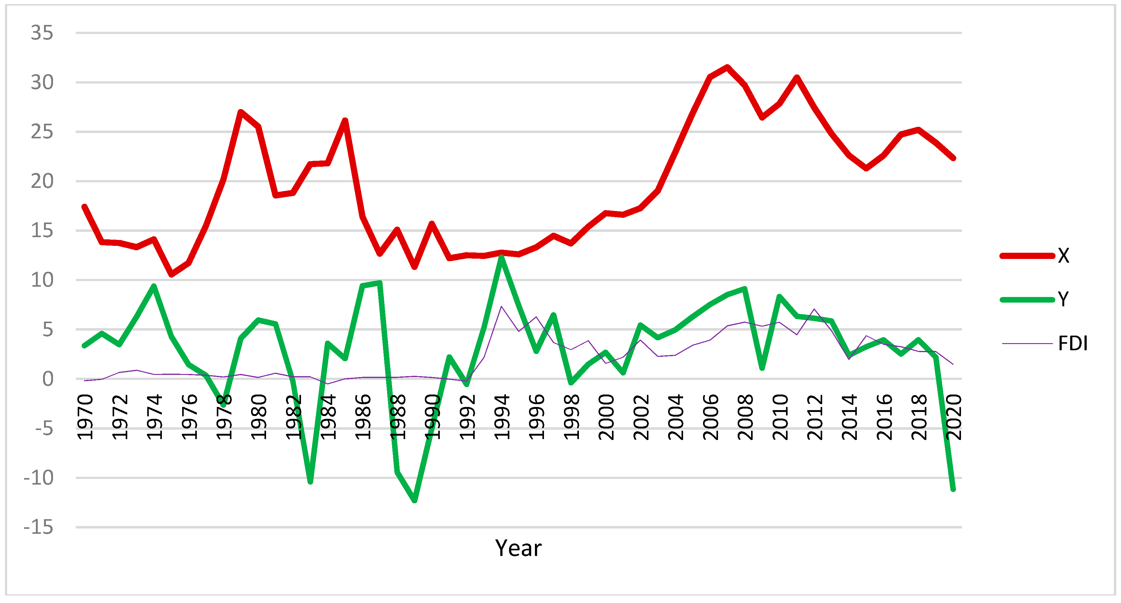
Figure 1 shows that the GDP growth rate follows a downward trend as of 2010; FDI oscillated around zero during the period 1970–1992, and exports also revealed a downward trend as of 2007 after an upward trend during the period 1991–2006.

2.3. Methodology

To establish the order of integration of the annual time series, the Dickey–Fuller unit root test (Dickey and Fuller 1979) must be applied by selecting any of its three auxiliary models (with trend and intercept, with intercept, and without trend or intercept). The auxiliary models can be corrected for the presence of higher-order autocorrelation of errors by selecting the optimal lag according to the Akaike (AIC), Schwarz Bayesian (SIC), and Hannan–Quinn (HQ) information criteria, whose null hypothesis expresses the presence of unit root in the series and the hypothesis test will consider the comparison of the $\tau$-statistic with any corresponding critical values of the Dickey–Fuller distribution.

The nonstationary series will be transformed into stationary series with the difference operator according to the order of integration resulting from the previous test. To determine causal relationships between the stationary series, the Granger causality test (Granger 1969) is applied, whose unrestricted auxiliary model presents the caused series as its regressand variable and as regressor variables to the lags of the same order for both caused and causing variables wherein the lag length will depend on the smallest value of the chosen information criterion (AIC, SIC, or HQ). The null hypothesis is the unidirectional noncausality between the stationary series and its F-statistic, with Fisher’s F probability distribution allowing hypothesis testing (Larios-Meoño and Álvarez-Quiroz 2014).

To evaluate the presence of cointegration between time series of integrated processes I(0) or I(1) in an autoregressive distributed lagged model (ARDL):

$$ARDL\left(p,q\right): Z_t=\beta +{\displaystyle \sum }_{i=1}^p{\delta }_i{Z}_{t-i}+{\displaystyle \sum }_{i=0}^q{\varphi }_i{W}_{t-i}+{\epsilon }_t$$

(17)

The methodology of Pesaran et al. (2001) will be adopted, along with the application of the cointegration bound test, whose null hypothesis is the absence of cointegration between $Z_t$ and $W_t$, which will be rejected when its $F$-statistic exceeds the bands $I\left(0\right)$ and $I\left(1\right)$. The existence of the long-term relationship between $Z_t$ and $W_t$ leads to the short-term analysis in its respective ECM from Equation (17). The estimated ECM should comply with the assumptions of the linear regression model (Larios-Meoño et al. 2016). Later, the Durbin–Watson first-order error autocorrelation test will be applied, and its d-statistic should be near 2 for the suspected absence of autocorrelation. The Breusch–Godfrey higher order autocorrelation test of errors incorporates the lags of the residual as additional regressor variables—considering the smallest value of the chosen information criterion—in its auxiliary model. In this model, the regressor is the contemporaneous residual, and the null hypothesis of absence of autocorrelation will be tested with its $LM$-statistic, which presents distribution probability ${\chi }^2$ with degrees of freedom equal to the lag length. The Breusch–Pagan–Godfrey, White, Harvey, and Glejser error heteroscedasticity tests indicate a null hypothesis with the presence of homoscedasticity of errors in the model; each one presents its $LM$-statistic with distribution probability ${\chi }^2$ with degrees of freedom equal to the number of regressor variables in their respective auxiliary models. The Jarque–Bera normality test applied to the residuals indicates a null hypothesis with the presence of normal probability distribution of residuals that will be tested through $JB$-statistic with distribution probability ${\chi }^2$ with degrees of freedom equal to 2. The Dickey–Fuller unit root test applied to the residuals with auxiliary model without constant or trend indicates a null hypothesis with the presence of unit root in the residuals and will be tested with the $\tau$-statistic that presents Dickey–Fuller distribution; the structural stability will be evaluated through the CUSUM and CUSUM of squares tests.

3. Results

In this section, we describe and interpret the results of statistical tests and econometric estimations performed in this article.

3.1. Unit Root Tests

The application results of the augmented Dickey–Fuller unit root test to the three series and their respective first difference transformations are presented in

Table 3. Results of augmented Dickey–Fuller unit root test.

Series	Auxiliary Model	Criteria *	Lag	$\mathit{\tau }$-Statistic	Probability	Integration **
$Y_t$	None	SIC	0	−3.41486	0.00100	$I\left(0\right)$
$X_t$	None	SIC	0	−0.30153	0.57210	$I\left(1\right)$
$\Delta X_t$	None	SIC	0	−6.31486	0.00000	$I\left(0\right)$
$FD{I}_t$	None	SIC	0	−1.54138	0.11460	$I\left(1\right)$
$\Delta FD{I}_t$	None	SIC	0	−8.86946	0.00000	$I\left(0\right)$

Prepared by the authors. (*) Schwarz Bayesian information criteria. (**) Integration order at 5% significance level.

.

From Table 3, it can be concluded that the series $X_t$ and $FD{I}_t$ are nonstationary series. The series transformed into first differences $\Delta X_t$ and $\Delta FD{I}_t$ are stationary series, as is the series $Y_t$ that did not require the application of the difference operator. Additionally, their Jarque–Bera statistics are 5.46718, 2.19097, and 21.29977, respectively, evidencing that $Y_t$ is the only stationary series that does not present normal probability distribution at the 5% significance level.

3.2. Granger Causality

The Granger causality test was used to evaluate the causal relationship between variables. It requires all variables to be stationary, $I\left(0\right).$ 

Table 4. Results of Granger’s causality test.

Causality *	Criteria	Lag	$\mathit{F}$-Statistics	p-Value
$\Delta FD{I}_t\to Y_t$	SIC **	2	3.69140	0.03360
$\Delta X_t\to Y_t$	SIC **	2	4.74714	0.01370
$Y_t\to \Delta X_t$	SIC **	3	3.52119	0.02350

Prepared by the authors. (*) 5% significance level. (**) Schwarz Bayesian information criteria.

shows the existence of unidirectional causality between $\Delta FD{I}_t$ and $Y_t$ and bidirectional causality between $\Delta X_t$ and $Y_t$ at the 5% significance level. Therefore, in the sense of Granger causality, our empirical evidence reveals confirmation of the FDI-led growth and feedback hypotheses between GDP and exports in Peru, both at the 5% significance level.

3.3. ARDL Cointegration

Table 4 evidences the endogeneity of $Y_t$ as variable $I\left(0\right)$ and the exogeneity of variables $I\left(1\right):$ $\Delta X_t$ and $\Delta FD{I}_t$. These integrated processes help in the estimation of the $ARDL\left(4,1,3\right)$ model with constant and trend, where $Y_t$ is the dependent variable, $X_t$ is the first independent variable, and $FD{I}_t$ is the second independent variable. Moreover, the lag length is attributed to the Akaike information criterion considering a maximum of 5 lags in all variables. The application of the unrestricted cointegration bound test in constant and restricted in trend on the estimated model $ARDL\left(4,1,3\right)$ yielded an $F$-statistic equal to 8.11543 and allowed the null hypothesis to be rejected at the 5% significance level. This was possible as band $I\left(0\right)$ is equal to 3.88 and band $I\left(1\right)$ is equal to 4.61, and in the long-term equilibrium, $X_t$ impacts $Y_t$ with a value of 0.18 and $FD{I}_t$ impacts $Y_t$ with a value of 1.64. The finding of the Pesaran–Shin–Smith long-term equilibrium relationship between the variables $Y_t$, $X_t,$ and $FD{I}_t$ led to the estimation of the respective ECM.

Table 5. Estimation of error correction model.

Variables	Coefficients
Constant	0.38236
Error correction term	−1.72142 *
$\Delta Y_{t-1}$	0.91856 *
$\Delta Y_{t-2}$	0.46843 *
$\Delta Y_{t-3}$	0.36176 *
$\Delta X_t$	−0.04461
$\Delta FD{I}_t$	1.44480 *
$\Delta FD{I}_{t-1}$	−0.77884
$\Delta FD{I}_{t-2}$	−0.88720 *
Regressand variable	$\Delta Y_t$
Observations	47
Number of coefficients **	9
$R^2$-adjusted	0.55437
$\mathrm{Probability}F$-statistic	0.00000
$\mathrm{Durbin}\text{–}\mathrm{Watson}d$-statistic	1.84239
$\mathrm{Breusch}\text{–}\mathrm{Godfrey}\mathrm{Prob}.LM$-statistic ***	0.85420
$\mathrm{Breusch}\text{–}\mathrm{Pagan}\text{–}\mathrm{Godfrey}\mathrm{Prob}.LM$-statistic	0.29168
$\mathrm{White}\mathrm{non}\text{-}\mathrm{cross}\mathrm{terms}\mathrm{Prob}.LM$-statistic	0.77760
$\mathrm{Harvey}\mathrm{Prob}.LM$-statistic	0.08332
$\mathrm{Glejser}\mathrm{Prob}.LM$-statistic	0.09135
$\mathrm{Jarque}\text{–}\mathrm{Bera}\mathrm{Prob}.JB$-statistic	0.44784
$\mathrm{Dickey}\text{–}\mathrm{Fuller}\mathrm{Prob}.\tau$-statistic ****	0.00000
$\mathrm{Cointegration}\mathrm{bound}\mathrm{test}F$-statistic *****	8.11543

Authors. (*) Statistically significant at 10% level. (**) Included constant. (***) Schwarz Bayesian information criteria and first-order lag. (****) Nonaugmented auxiliary model by Schwarz Bayesian information criteria. (*****) Unrestricted constant and restricted trend.

shows the results of the estimated ECM with a significant and negative coefficient of the error correction term supporting the results of the long-term equilibrium relationship; a significant and positive short-term impact on $\Delta Y_t$ is caused by $\Delta FD{I}_{t-2}$, and a nonsignificant short-term impact on $\Delta Y_t$ is caused by $\Delta X_t$. Goodness-of-fit is preserved in the estimated ECM with an $R^2$-adjusted greater than 0.5. There is a joint statistical significance between the slope coefficients at 5% and suspicion of no first-order autocorrelation of residuals due to the Durbin–Watson d-statistic value being close to 2. The results of the Breusch–Godfrey error higher order autocorrelation test confirm that the model residuals at the 5% significance level do not exhibit first-order autocorrelation according to the Schwarz Bayesian information criteria. The homoscedasticity of model residuals is guaranteed at the 5% significance level according to the results of the Breusch–Pagan–Godfrey, White (non-cross terms), Harvey, and Glejser tests. Additionally, the model residuals present normal probability distribution at the 5% significance level according to the results of the Jarque–Bera normality test. The Dickey–Fuller unit root test of the residuals expresses that they constitute a process $I\left(0\right)$ at the 5% significance level, and structural stability is confirmed at the 5% significance level with the CUSUM and CUSUM of squares tests.

4. Discussion

The Granger causality analysis gave us the following two findings. First, the FDI-led growth theoretical hypothesis is confirmed for the Peruvian economy, coinciding in one direction with Oladipo (2013), who found the feedback hypothesis between FDI and GDP growth rate in Peru. Additionally, we find the feedback relationship between GDP and exports.

The cointegration analysis between the three variables GDP, exports, and FDI—meaning the long-term equilibrium relationship between them, where GDP is the dependent variable—allowed us to find the following two outstanding results. First, exports have a positive long-term equilibrium impact and less than unity on GDP. Second, FDI has a long-term equilibrium impact greater than unity on GDP. On the other hand, Bustamante (2017) found a long-term equilibrium inelastic behavior from FDI to GDP for Peru. Herzer et al. (2008) also found a statistically strong long-term equilibrium relationship between the logarithm of GDP and FDI-to-GDP ratio in Peru.

The presence of cointegration has required the estimation of the error correction model as a short-term relationship between the three variables GDP, exports, and FDI that allow us to obtain the following two results. First, the exports have no significant short-term impact on GDP. Finally, FDI has a short-term impact greater than one with respect to GDP.

According to the theoretical model—the Mundell–Fleming static model with specific assumptions adopted in our study—the implicit function theorem applied in the system of implicit functions that come from the equilibrium of the three markets involved in this article, we specify two important comparative static derivates obtained from equilibrium implicit function of GDP. The comparative static derivate from exports to GDP explains that the changes in exports have no effect on the GDP. The other comparative static derivate expresses that the change in FDI increases the GDP when the slope of curve LM is greater than the slope of curve IS, and the change in FDI decreases the GDP when the slope of curve LM is lower than the slope of curve IS. Obviously, the empirical results may or may not agree with theoretical results.

5. Conclusions

In this paper, the macro-econometric results of Peru are consistent with our three theoretical results obtained in the Mundell–Fleming statical model with specific assumptions, the increased FDI theoretically achieves a positive or negative variation of GDP as long as the slope of the curve $IS$ is greater or lower than the slope of the curve $LM$, but the increase in exports does not theoretically affect GDP. Empirically, the Granger causality and the dynamic impacts—both in short and long terms—of FDI on the country’s economic growth have been therefore demonstrated, and we conclude that the FDI-led Growth hypothesis if fulfilled in Peru; thus, the increase in FDI produces—in the short and long-term—an increase in GDP at a higher rate, i.e., the GDP has an elastic behavior regarding FDI; also, the change in the exports increases at a lower rate to GDP in the long-term equilibrium, but only in the short-term do exports have a statistically insignificant effect on GDP. Table 1 shows an increase in average real GDP, exports, and FDI during 1970–2020, in general, due to the economic stability of the country, but it should be noted that FDI has grown at a lower rate in the last years due to the political crisis. Peru’s economic policy path should continue to attract foreign capital to increase FDI, which, in turn, will facilitate greater economic growth that ought to translate into social development and welfare.

References

- Abbes, Sahraoui Mohammed, Belmokaddem Mostéfa, Guellil Mohammed Seghir, and Ghouali Yassine Zakarya. 2015. Causal Interactions Between FDI, and Economic Growth: Evidence from Dynamic Panel Co-integration. Procedia Economics and Finance 23: 276–90. [Google Scholar] [CrossRef]
- Akoto, William. 2016. On the Nature of the Causal Relationships Between Foreign Direct Investment, GDP and Exports in South Africa: FDI, GDP and Exports in South Africa. Journal of International Development 28: 112–26. [Google Scholar] [CrossRef]
- Andraz, Jorge Miguel, and Paulo Manuel Marques Rodrigues. 2010. What Causes Economic Growth in Portugal: Exports or Inward FDI? Journal of Economic Studies 37: 267–87. [Google Scholar] [CrossRef]
- Baliamoune-Lutz, Mina. 2004. Does FDI Contribute to Economic Growth? Business Economics 39: 49–56. [Google Scholar]
- Barro, Robert Joseph. 1990. Government Spending in a Simple Model of Endogenous Growth. Journal of Political Economy 98, Part 2: S103–S125. [Google Scholar] [CrossRef]
- Bazán, Ciro, Víctor Josué Álvarez-Quiroz, and Yennyfer Morales Olivares. 2022. Wagner’s Law vs. Keynesian Hypothesis: Dynamic Impacts. Sustainability 14: 431. [Google Scholar] [CrossRef]
- Belloumi, Mounir. 2014. The Relationship Between Trade, FDI and Economic Growth in Tunisia: An Application of The Autoregressive Distributed Lag Model. Economic Systems 38: 269–87. [Google Scholar] [CrossRef]
- Blanchard, Olivier. 2021. Macroeconomics, 8th ed. Harlow: Pearson. [Google Scholar]
- Borensztein, Eduardo, José de Gregorio, and Jong-Wha Lee. 1998. How does Foreign Direct Investment Affect Economic Growth? Journal of International Economics 45: 115–35. [Google Scholar] [CrossRef]
- Bustamante, Rafael. 2017. La Inversión Extranjera Directa en el Perú y sus Implicancias en el Crecimiento Económico 2009–2015. Pensamiento Crítico 21: 051–63. [Google Scholar] [CrossRef]
- Central Reserve Bank of Peru. 1990. Memoria Anual. Available online: https://www.bcrp.gob.pe/publicaciones/memoria-anual/memoria-1990.html (accessed on 2 May 2022).
- Central Reserve Bank of Peru. 1995. Memoria Anual. Available online: https://www.bcrp.gob.pe/publicaciones/memoria-anual/memoria-1995.html (accessed on 2 May 2022).
- Central Reserve Bank of Peru. 2015. Memoria Anual. Available online: https://www.bcrp.gob.pe/publicaciones/memoria-anual/memoria-2015.html (accessed on 2 May 2022).
- Central Reserve Bank of Peru. 2020. Memoria Anual. Available online: https://www.bcrp.gob.pe/publicaciones/memoria-anual/memoria-2020.html (accessed on 2 May 2022).
- Central Reserve Bank of Peru. 2021. Memoria Anual. Available online: https://www.bcrp.gob.pe/publicaciones/memoria-anual/memoria-2021.html (accessed on 2 May 2022).
- de la Fuente, Angel. 2000. Mathematical Methods and Models for Economists. Cambridge: Cambridge University Press. [Google Scholar]
- de Mello, Luiz. 1997. Foreign Direct Investment in Developing Countries and Growth: A Selective Survey. Journal of Development Studies 34: 1–34. [Google Scholar] [CrossRef]
- Dickey, David Alan, and Wayne Arthur Fuller. 1979. Distribution of the Estimators for Autoregressive Time Series with a Unit Root. Journal of the American Statistical Association 74: 427. [Google Scholar] [CrossRef]
- Dornbusch, Rudiger, Stanley Fischer, and Richard Startz. 2018. Macroeconomics, 13th ed. New York: McGrawHill. [Google Scholar]
- Dritsaki, Chaido, and Emmanouil Stiakakis. 2014. Foreign Direct Investments, Exports, and Economic Growth in Croatia: A Time Series Analysis. Procedia Economics and Finance 14: 181–90. [Google Scholar] [CrossRef]
- Fleming, John Marcus. 1962. Domestic Financial Policies under Fixed and under Floating Exchange Rates. Staff Papers—International Monetary Fund 9: 369. [Google Scholar] [CrossRef]
- Gandolfo, Giancarlo. 2016. International Finance and Open-Economy Macroeconomics. Berlin and Heidelberg: Springer. [Google Scholar] [CrossRef]
- Granger, Clive William John. 1969. Investigating causal relations by econometric models and cross-spectral methods. Econometrica 37: 424–38. [Google Scholar] [CrossRef]
- Herzer, Dierk, Stephan Klasen, and Felicitas Nowak-Lehmann. 2008. In Search of FDI-Led Growth in Developing Countries: The Way Forward. Economic Modelling 25: 793–810. [Google Scholar] [CrossRef]
- Hobbs, Sam, Dimitrios Paparas, and Mostafa AboElsoud. 2021. Does Foreign Direct Investment and Trade Promote Economic Growth? Evidence from Albania. Economies 9: 1. [Google Scholar] [CrossRef]
- Hsiao, Frank, and Mei-Chu Hsiao. 2006. FDI, Exports, and GDP In East and Southeast Asia—Panel Data Versus Time-Series Causality Analyses. Journal of Asian Economics 17: 1082–106. [Google Scholar] [CrossRef]
- Jiménez, Félix. 2006. Macroeconomía: Enfoques y Modelos. Lima: Pontifica Universidad Católica del Perú, vol. 1, Available online: https://departamento.pucp.edu.pe/economia/libro/macroeconmia-enfoques-y-modelos-tomo-i/ (accessed on 3 June 2022).
- Larios-Meoño, José Fernando, and Víctor Josué Álvarez-Quiroz. 2014. Fundamentos de Econometría. Fondo Editorial USIL. Available online: https://fondoeditorial.usil.edu.pe/publicacion/fundamentos-de-econometria/ (accessed on 5 June 2022).
- Larios-Meoño, José Fernando, Carlos González-Taranco, and Víctor Josué Álvarez-Quiroz. 2016. Investigación en Economía y Negocios: Metodología con Aplicaciones en E-Views. Fondo Editorial USIL. Available online: https://fondoeditorial.usil.edu.pe/publicacion/investigacion-en-economia-y-negocios-metodologia-con-aplicaciones-en-e-views/ (accessed on 5 June 2022).
- Lucas, Robert Emerson. 1988. On the Mechanics of Economic Development. Journal of Monetary Economics 22: 3–42. [Google Scholar] [CrossRef]
- Malaspina, Ulda junerico. 1994. Matemáticas para el Análisis Económico, 1st ed. Lima: Fondo Editorial de la Pontificia Universidad Católica del Perú. [Google Scholar]
- Mundell, Robert Alexander. 1963. Capital Mobility and Stabilization Policy under Fixed and Flexible Exchange Rates. The Canadian Journal of Economics and Political Science 29: 475. [Google Scholar] [CrossRef]
- Nguyen, Nhung Thi Kim. 2017. The Long Run and Short Run Impacts of Foreign Direct Investment and Export on Economic Growth of Vietnam. Asian Economic and Financial Review 7: 519–27. [Google Scholar] [CrossRef] [Green Version]
- Oladipo, Olajide. 2013. Does Foreign Direct Investment Cause Long Run Economic Growth? Evidence from the Latin American and the Caribbean Countries. International Economics and Economic Policy 10: 569–82. [Google Scholar] [CrossRef]
- Parkin, Michael, and Robin Bade. 2016. Macroeconomics: Canada in the Global Environment, 9th ed. Toronto: Pearson. [Google Scholar]
- Pesaran, Mohammad, Yongsheol Shin, and Richard Smith. 2001. Bounds Testing Approaches to The Analysis of Level Relationships. Journal of Applied Econometrics 16: 289–326. [Google Scholar] [CrossRef]
- Romer, Paul. 1986. Increasing Returns and Long-Run Growth. Journal of Political Economy 94: 1002–37. [Google Scholar] [CrossRef]
- Romer, Paul. 1993. Idea Gaps and Object Gaps in Economic Development. Journal of Monetary Economics 32: 543–73. [Google Scholar] [CrossRef]
- Sarker, Bibhuti, and Farid Khan. 2020. Nexus Between Foreign Direct Investment and Economic Growth in Bangladesh: An Augmented Autoregressive Distributed Lag Bounds Testing Approach. Financial Innovation 6: 10. [Google Scholar] [CrossRef]
- Sharmiladevi, Jekka Chandrasekaran. 2020. Cointegration and Causality Study Among Inward FDI, Economic Growth and Exports: An Indian Perspective. International Journal of Asian Business and Information Management 11: 63–77. [Google Scholar] [CrossRef]
- Solow, Robert Merton. 1956. A Contribution to the Theory of Economic Growth. The Quarterly Journal of Economics 70: 65. [Google Scholar] [CrossRef]
- Sopta, Martina, Vlatka Bilas, and Sanja Franc. 2021. Cointegration and Causality Analysis Between Foreign Direct Investment, Exports and Economic Growth in The Republic of Croatia. Management 26: 145–58. [Google Scholar] [CrossRef]
- Sultanuzzaman, Md Reza, Hongzhong Fan, Mahamud Akash, Banban Wang, and Uddin Sarker Md Shakij. 2018. The Role of FDI Inflows and Export on Economic Growth in Sri Lanka: An ARDL Approach. Cogent Economics & Finance 6: 1518116. [Google Scholar] [CrossRef]
- Sydsæter, Knut, and Peter Hammond. 2008. Further Mathematics for Economic Analysis, 2nd ed. Harlow: Pearson. [Google Scholar]
- Szkorupová, Zuzana. 2014. A Causal Relationship between Foreign Direct Investment, Economic Growth and Export for Slovakia. Procedia Economics and Finance 15: 123–28. [Google Scholar] [CrossRef] [Green Version]
- Takayama, Akira. 1994. Analytical Methods in Economics. New York: Harvester Wheatsheaf. [Google Scholar]
- Tanaya, Olivia, and Suyanto Suyanto. 2022. The Causal Nexus Between Foreign Direct Investment and Economic Growth in Indonesia: An Autoregressive Distributed Lag Bounds Testing Approach. Periodica Polytechnica Social and Management Sciences 30: 57–69. [Google Scholar] [CrossRef]
- The World Bank. 2022. Indicators. Available online: https://data.worldbank.org/indicator?tab=all (accessed on 5 May 2022).
- Wang, Peijie. 2020. The Economics of Foreign Exchange and Global Finance, 3rd ed. Berlin: Springer. [Google Scholar]
- Yao, Shujie. 2006. On Economic Growth, FDI and Exports in China. Applied Economics 38: 339–51. [Google Scholar] [CrossRef]
- Zhang, Kevin Honglin. 2001. Does Foreign Direct Investment Promote Economic Growth? Evidence From East Asia and Latin America. Contemporary Economic Policy 19: 175–85. [Google Scholar] [CrossRef]
Figure 1.
Export, Foreign Direct Investment and GDP growth rate, 1970–2020, Peru. Prepared by the authors.