Abstract
The “technology bubble” in the late 1990s, the financial crisis in 2007/2008, and the Eurozone crisis generated significant losses across several asset classes. The objective of this paper is to investigate risk premia factors such as size, value, momentum, carry, quality, and low volatility and their time-variant behavior. The time-variant behavior of these risk premia baskets has been analyzed based on different financial conditions: The business cycle, the yield curve, equity market momentum, and different risk conditions. Factor calculations are based on the MSCI World universe. The monthly data set ranges from January 1995 to September 2017. The results underpin the prevalent observation that equity risk factors consistently outperform the broad market and therefore generate significant alpha. However, the paper shows that a dynamic allocation of risk factors can achieve an attractive return–risk relation. The study shows very clearly how different risk factors behave in different financial conditions and that an allocation to more offensive or more conservative risk factors can outperform a diversified, equally-weighted portfolio.
1. Introduction
Uncertainty and unforeseen market movements are not unusual in financial markets. The “technology bubble” in the late 1990s, the financial crisis of 2007/2008, and the Eurozone crisis are three recent examples. These crises generated dramatic losses in equity value and ultimately leads to doubts about the benefits of equity risk factor diversification. This leads to the question whether dynamic factor allocation generates an outperformance compared to an equally weighted factor portfolio?
Dynamic factor allocation or “factor timing” is an area of academic and practical research. The objective of this paper is to present the risk drivers behind equities and to demonstrate that equities earn risk premiums because they are exposed to underlying risk factors and asset classes are bundles of those factor risks. The final focus will be on the construction of risk factor portfolios.
In addition, the work assesses the robustness and the field of application of equity risk premia in portfolio management. This paper builds on conclusions drawn by current academic research. This research makes the following contributions: Firstly, by using a dynamic risk premium approach, it will be illustrated that the previously static- and diversification-based academic papers should be expanded by a dynamic component. Secondly, it focuses on six risk premia strategies namely size, value, momentum, carry, quality, and low volatility, and the risk and return characteristics of these risk premia have been investigated. Thirdly, factor timing strategies concerning the business cycle, interest rate cycle and risk environment have been developed accordingly. Furthermore, behavioral finance and neo-classical explanations are shown in the Table 1.

Table 1.
Behavioral finance and neo-classical explanations.
In this regard, the major finding is a close link between the business cycle and the prevalent risk regime, where economic expansion coincides with decreasing risk aversion and economic downturns lead to increased risk aversion. However, the business cycle strategy exhibits by far the most attractive return–risk relation.
2. Literature Review of Dynamic Factor Allocation
A large body of academic research has supported the dynamic allocation between different asset classes—the asset allocation decision. Asset allocation is understood as the efficient and optimal allocation of different asset classes considering the investor’s utility function, or risk and return preferences. Asset allocation is the investment in different asset classes across market regimes and across time. Gügi (1996) took the view that both practice and academic literature distinguish between strategic, tactical, and dynamic asset allocation. However, the allocation between different equity risk factors has not yet been investigated satisfactorily. According to Schneeweis et al. (2010), the goal of tactical asset allocation (TAA) is to generate a long-term alpha and a short-term improvement of the risk–return characteristics of the portfolio compared to the strategic asset allocation by changing allocations within and between asset classes. More specifically, this means that, following Schneeweis et al. (2010), the investor has to assess the expected return of asset class , the current macro-economic changes as well as fundamental changes :
TAA is, therefore, proactive and anticipates the behavior of markets. Dynamic factor timing should be understood as being analogous to the tactical asset allocation process. Harvey (1989) showed that equity risk premia are higher at business cycle troughs and lower at peaks. Cochrane and Piazzesi (2005) found that term premia vary over time and show countercyclical movements, which is also valid for exchange rate risk premia, according to Lustig and Verdelhan (2007). According to Campbell and Cochrane (1999) as well as Bansal and Yaron (2004), the two most well-known asset pricing models attribute this variation to countercyclical changes in risk aversion and the volatility of the consumption process. The research that equity risk premia vary over time is to be understood as legitimization for the tactical asset allocation and dynamic risk factor timing. As Bender et al. (2017) stated, factor premia are compensation for exposure to risk and the components are highly time-varying, which explains the time-variance for factor premia. Examples of this are quality (high ROE and ROA with low debt) and low volatility stocks, which were the best performing factors in the last 5 years, but the worst performers in the bull market until 2008. Bender et al. (2017) findings show that sentiment is closely related to financial conditions and the general economic environment. Additionally, the US term spread can be used as an indicator for weakening economic conditions. The steepest yield curve can be usually found during a recession in which investors require higher compensation for risk-seeking assets. Therefore, defensive assets are likely to underperform when approaching a recession. It is important to note the time horizon for the different predictors. For example, unit-output growths, personal savings rate, CPI and PPI, have strong correlations with value and investment factors at 1-year horizons. The TED spread and term spread are strong predictors for horizons greater than 6 months, particularly for the factor’s value, profitability, investment, and momentum.
Additionally, the researchers also found a significant problem with those predictors, as they have time-varying relationships. For example, widening credit spreads preceded a good performance of the value factor in 2000–2001, but a poor performance in 2008–2009. These findings indicate that predictors that were accurate in the past might not be accurate in the future due to changes in other variables in the economy. A similar finding was shown by Dai (2017), who conducted a multivariate regression analysis using different bond yields and size, value, and profitability premiums. The resulting R2 (a measure of explanatory power) was close to zero, which led Dai (2017) to conclude that there is no robust relationship between interest rate changes and the size, value, and profitability premiums.
The researchers did not specify the predicting explanatory variables that should be used but referred to those in the existing literature (e.g., Federal Reserve discount-rate changes Jensen et al. 1996) or the ratio of book value to the market value of common equity (Chan et al. 1998). This asset allocation included the four Russel indexes and other asset classes such as bonds. Within the model, they derived the probability that a particular style index will outperform another index. Based on these probabilities, they weighted the indexes or other asset classes in their portfolio, following several trading strategies (both single style and mixed style). After making further improvements to their trading strategies, by implementing probability thresholds, the best strategies were able to significantly outperform the S&P 500.
A study by Bird and Casavecchia (2008) demonstrated that macroeconomic and market factors were able (monthly) to predict the direction of the value premium over the next 12 months. The macroeconomic indicators used here were unexpected inflation, the Baa–Aaa bond yield spread, the dividend yield on European equities, the change in the steepness of the yield curve (10Y-3M), and the change in the inflation-adjusted 3-month Treasury bill. Using their regression model, they achieved a forecasting ability of 70% for the next 12 months to switch between their value and growth portfolios. This finding supports the hypothesis proposed by Bender et al. (2013) that time horizons do play an important role.
According to Asness et al. (2017), implementing a successful contrarian timing strategy is harder in practice and against relevant alternatives (diversified portfolios). His studies showed that value spreads indeed have a mean-reverting nature, which suggests that style timing would be possible. However, closer examination of the nature of style valuation reveals that changes in style valuation are due to changes in portfolio positions or fundamentals, rather than prices. Hence, if the value style reverts to the mean, for example, this reversion should not be expressed through changes in prices, which makes style timing unnecessary. When exploring the timing for multi-style portfolios, it is important to recognize that the correlations between the different styles may contradict each other. An increase in the performance of momentum should usually occur at the expense of the value style, as assets will have improved in price. Having a negative correlation, Asness et al. (2017) compared the performance of a multi-style portfolio (combining value and momentum) with and without value timing. They used the z-score of the book-to-price spread for each style as a timing signal. The comparison showed no significant performance improvement in that regard.
Asness et al. (2000) showed that expected return premiums can vary through time as a consequence of rational or irrational forces. To achieve that, they used the following valuation measures: earnings-to-price, book-to-price, and sales-to-price. After adjusting those measures for different industries, they ranked the stocks for each measure and weighted them based on their average rank. As a measure for growth, they used the IBES median long-term EPS growth forecast at time t. The spreads of these measures (between growth and value) were used to forecast returns. In the course of a regression, between the actual returns and the predicted returns, had a low value, which indicates that the model has low explanation power.
Arnott et al. (2017) described “smart beta” timing as “easy” and even implied that the majority of market participants already do it without realizing it. The underlying methodology to that hypothesis is a comparison between “trend-chasing” smart beta strategies (the best performers in the recent time periods) and contrarian strategies (worst performers of the recent time periods). The strategies consisted of 7 indexes (each index included a set of 1000 US stocks) representing different factors or styles. The results showed the relative outperformance of the contrarian strategies against the trend-chasing strategies with the same volatility over the time horizons from 1, 3, 5, and 10 years. This supports the thesis of Asness et al. (2017) that styles or factors do indeed have a mean-reverting nature.
Finally, it can be concluded that there are models that can predict future premia and can therefore help the timing of certain factors. A definite disadvantage is that there will always be some uncertainty since indicators that have worked in the past (and therefore also models) might not be accurate predictors for the future. Some studies have demonstrated that factor timing is possible for a given time horizon. These models are mostly reliant on macroeconomic data and use already existing indexes in their portfolios.
Empirical Evidence on Risk Premia Factors
The most well-known factors among investors are market, size, value, and momentum. Fama and French (1992) documented value and size, whereas Jegadeesh and Titman (1993) and Carhart (2012) investigated momentum. These factors were documented by Ang et al. (2009); Blitz and van Vliet (2008); Huji and Verbeek (2009). However, these articles investigated size, value, and momentum factors, as well as market factors. Ilmanen (2016) studied value, momentum, carry, and quality. Bender et al. (2013) investigated the same six factors (size, value, momentum, carry, quality, and low volatility) to measure the attractiveness of one individual stock concerning a specific factor. All these factors consistently provided positive returns. Thus, the equity premium is documented by the empirical evidence (e.g., Dimson et al. 2016). This study focuses on six factors following Bender et al. (2013).
De Bondt and Thaler (1985, 1987) documented that long-term past losers would outperform long-term past winners. Jegadeesh (1990) and Lehmann (1990) stated that stocks selected based on the previous week’s or month’s return tend to outperform others. Moskowitz and Grinblatt (1999) documented momentum effects at the industrial level. Daniel and Moskowitz (2013) found so-called “momentum crashes” and documented a high tail risk in momentum strategies, which was a sign that momentum could be defined as a risk factor. Pastor and Stambaugh (2003) explained the momentum returns with liquidity risk and Asness et al. (2013) showed a strong correlation among momentum stocks and interpreted this as a common source of a risk factor. Barberis et al. (1998) as well as Hong and Stein (1999) investigated the underreaction phenomenon and justified momentum with the short-term underreaction of market participants when processing information. Hirshleifer (2001) and Barberis and Thaler (2003) explained the anomaly by an underreaction to earnings announcements and news or a delayed reaction Backhaus and Isiksal (2016). Momentum would continue as a “pervasive phenomenon” until there would be large deviations from the fundamental price as a result of market reversals and this confirmed the existence of the value factor (Vayanos and Woolley 2013).
Graham and Dodd (1934) set the foundations of value investing with their book “Security Analysis”. Asness et al. (2015) demonstrated that higher risk-adjusted returns are the result of leverage constraints regarding value. Zhang (2005) argued that companies with low valuations are unable to respond to flexibly unforeseen environmental trends as companies with a high valuation. Therefore, investors need an additional premium as a form of risk compensation. Koijen et al. (2017) showed that value premium is compensation for macroeconomic risk.
Historically, under normal market conditions, low volatility stocks have performed in line with high volatility stocks; however, during market crises, investors seek safer assets and low volatility stocks tend to outperform as a result. Option-like behavior is often cited as a reason for the premium, and hence, the outperformance of low volatility stocks. The robustness of the volatility premium was confirmed by Chan et al. (1999); Jagannathan and Ma (2003); Clarke et al. (2006). The low beta premium reveals that low beta stocks outperform high beta stocks (Baker et al. 2011). Frazzini and Pedersen (2014) confirmed the low beta phenomenon.
Koijen et al. (2017) found that the carry strategy was not correlated with value and momentum strategies. Additionally, carry predicts returns in cross-sectional and time-series data for different asset classes such as equities, bonds, and commodities. Koijen et al. (2017) defined the carry of a futures contract as the expected return if the spot price does not change over the holding period. Israel and Maloney (2014) showed that higher-yielding assets provide higher returns than lower-yielding assets and supported the risk hypothesis which contradicts the pure expectation and uncovered interest rate parity hypothesis. Based on historical data analysis, carry strategies suffer from large drawdowns in periods of market distress and liquidity risk and exhibit tail risks (Roncalli 2017). Binsbergen et al. (2012) and Ahmerkamp and Grant (2013) demonstrated that variables known to be related to the business cycle such as default spread, term spread, and T-bill yield could predict carry returns. These findings and the vast amount of empirical research regarding currency carry trades, such as Brunnermeier et al. (2008), have shown that carry returns are related to the business cycle and to recession and expansion periods, which confirms that carry returns are a compensation for time-varying risk premia. Pastor and Stambaugh (2003) detected the liquidity risk inherent in carry strategies. Bansal et al. (2014) showed the volatility risk of carry trades and Lettau et al. (2014) showed the downside risk exposure. Overall, carry strategies are affected by different risk factors, and therefore the assumption of the risk premium theory holds.
Quality is similar to value investing, according to Graham (1949). Graham (1949) selected low volatility stocks from companies with low leverage and stable earnings (quality companies). Based on the Barra style model, Goldberg et al. (2015) posited that the quality factor loads positively affect earnings yield and negatively on beta, residual volatility, and leverage factors. These findings were consistent with the profile of quality investing (Goldberg et al. 2015). Asness et al. (2015) defined quality as stocks that were safe, profitable, growing, and well-managed. Piotroski (2000) considered three dimensions of quality: profitability, leverage/liquidity, and operating efficiency. Norges Bank’s (2015) empirical evidence exhibited that high-quality stocks generated superior returns and they stated that it was unclear whether the quality premium was compensation for non-diversifiable risk.
Bali et al. (2016) examined the relationship between small-cap companies and expected stock returns and found that small-cap stocks strongly outperformed large caps. They demonstrated that the excess return was mainly driven by small-cap stocks. Leledakis et al. (2004) exhibited the excess return of small-sized companies in the UK market. Winkelmann et al. (2013) showed a higher sensitivity of small-cap stocks to economic shocks than large caps. Therefore, the premium was compensation for macroeconomic risk.
3. Empirical Investigation
Each factor reflects a distinct risk premium and has a clear economic rationale. We define six factors according to the following characteristics:
where and describe the stock price and the number of stocks outstanding at time t, respectively. This factor is referred to as the “small firm effect”, as smaller firms tend to outperform larger ones on a long-term horizon.
where
represents the book value per share, is a price per share. There are other value measures such as price-to-earnings, price-to-cash-flow, price-to-sales, etc. This study aims to search for a simple and transparent way of measuring risk premia. For this reason, the most popular version of the value measure was chosen, and individual stocks were ranked on a price-to-book basis.
The last month’s return is skipped due to reversal effects at the stock level and the momentum figure is calculated by dividing the price P at t − 1 by the stock price 12 months ago. The concept of momentum effect is that on average, past winners tend to outperform, while past losers keep underperforming.
The total return of a stock investment can be divided into two components: dividend yield and capital gains. The bird-in-hand theory states that investors prefer the certainty of dividend payments over the possibility of substantially higher future capital gains. Thus, stocks with high dividend payouts are sought by investors and consequently command a higher market price.
High earnings relative to book value mean higher profitability and thus, higher future growth in sales and earnings.
The low-volatility anomaly is the observation that portfolios of low-volatility stocks have higher risk-adjusted returns than portfolios with high-volatility stocks.
The universe consists of all stocks from the MSCI World index. The underlying benchmark for model backtesting will be represented by an equal-weighted factor index (strictly speaking, every single factor has a one-sixth weight) based on MSCI World factor indices. Rebalancing occurs at the end of each month. The stock returns and accounting data are retrieved from Datastream and Bloomberg. The sample period is based on monthly data starting in January 1995 and ending in September 2017. At the end of each quarter, all securities are ranked in ascending order according to their factor measure. Based on these rankings, ten decile portfolios are created where the stocks are equally weighted within the top decile, the second decile, and so on. The top decile portfolio is called the “losers” decile and the bottom decile is called the “winners” decile. Stocks in the fifth and sixth portfolios represent the “center” of the distribution. Since the universe comprises more than 1600 stocks in each case, each individual basket contains at least 160 securities (companies with negative book values are excluded).
For this research, the three bottom deciles are considered to fully capture the characteristics of each factor (long-only). The relevant return and risk characteristics of each factor are found in a sample that is much larger than one decile. In the case of significant differences between the first and subsequent portfolios, it would not be possible to conclude that a risk premium exists that continuously declines from best to worst portfolios. The reallocation procedure can be described as follows: every quarter, the strategy buys the three bottom portfolios and holds this position for the next three months. After three months, the next reallocation takes place, and a new factor portfolio is constructed that is held for the next three months. These steps reoccur until the end of the sample period.
Each factor portfolio is assessed by the following return and risk measures: return per annum, volatility per annum, return–risk ratio, and skewness. The skewness describes the degree of asymmetry of returns. Skewness is defined by the following equation:
Moreover, we calculate the beta of individual strategies (these strategies will be based on factor timing concerning price momentum, business cycle, yield curve, and risk regimes) concerning the equal-weighted factor index and test the resulting intercept (which can be interpreted as the factors alpha) for statistical significance. In this context, we run the following time series regression for the entire sample period:
and are the monthly returns of the relevant risk premium portfolio and the factor index, respectively. Under the null hypothesis, there is no existence (and therefore economic significance as well) of abnormal returns concerning one individual risk premium. In this case, the alpha, value would barely deviate from zero. In contrast, beta β describes the strength of co-movement of the factor concerning the factor index, is a risk-free rate and is the error term.
To analyze the different behavior of these risk premia baskets, the return characteristics in different market regimes have been investigated. As a starting point, market regimes based on business cycle phases have been defined. Therefore, a business cycle indicator has been created which captures four relevant phases of market activity. Since capital markets lead economic indicators by 6 to 9 months, it was decided to include only market movements into that cycle indicator.
The single indicators are derived from different classes and regions around the world. Their construction is based on the so-called z-score approach (one observation will be normalized by their historical mean and standard deviation) with a trailing window of 500 business days. The main groups that form the overall indicator are equity markets, bond markets, credit markets, and commodity markets. To obtain a comprehensive view of the business cycle, four phases that differ in level and change are defined. An optimal measure of change should be sufficiently fast to identify market highs and troughs immediately after they occur but should also exhibit low fluctuations to avoid false signaling. Hence, the 3-month change of the business cycle indicator was defined as the appropriate measure of change. The final phases resulting from these two measures can be classified as expansion (positive value, positive change), peak (positive value, negative change), recession (negative value, negative change), and recovery (negative value, positive change).
Following that classification, the return characteristics of the individual risk factors were examined as a function of the market regime. Therefore, the monthly return of each risk premium was allocated to the phase of the business cycle, which has been measured at the end of the prior month. Finally, the last step involves the creation of a factor rotation strategy that selects single factors based on the current business cycle stage. At the end of each month, the business cycle indicator determines the current phase. Based on this observation, three out of six factors are chosen concerning their return and risk characteristics shown in this phase. To obtain an impression of this superior selection tool, a momentum and a yield curve strategy have also been constructed. The former ranks risk premia according to their price momentum over a six- and nine-month horizon. The latter picks risk premia based on their return and risk characteristics shown in different interest rate cycles, as measured by the slope of the US yield curve. Thus, the range of yield curve slope realizations (roughly from −50 to 300 basis points within the observation period) was divided into four single areas.
Furthermore, we investigated style behavior among different risk regimes. The underlying analysis will be based on a macroeconomic risk indicator. The indicator measures stress in traditional risk-sensitive implied volatilities for FX options, equity options, and interest rates, three-month TED-spread, corporate CDS spreads as well as emerging market sovereign spreads. The indicator is available in the Bloomberg information system. Exchange rate volatility is measured by the 3-month implied volatility of different currencies. Equity market volatility is represented by the VIX and VSTOXX, the implied volatilities of the US and European equity markets, respectively. Interest rate volatility is measured by the volatility of European and US bond markets. The Ted-spread tracks the difference between the 3-month USD LIBOR and the yield on 3-month US T-Bills. Credit default swaps are used for European and US high yield markets. Emerging market spreads measure the premium of emerging market hard currency bonds versus US Treasury bonds. The overall risk indicator will be determined by the so-called “percentage rank procedure” on a single-indicator level with a trailing window of 250 business days. The respective strategy selects risk premia according to their return behavior in the prevailing risk environment. To remain consistent with the business cycle and yield curve classification, four phases were defined conditional on the current risk perception, which can be described as complacency, risk on, risk off and crash.
4. Empirical Results
Momentum (Table 2) realized an average return of 10.26% per annum and it has the lowest skewness, which is superior to the other factors. The return–risk ratio is quite remarkable. Small caps have the highest volatility among all factors. Value stocks have the lowest average return and the lowest return–risk ratio. Quality stocks deliver a promising return due to their less risky nature, whereas quality stocks exhibit smaller volatility and thus a superior return–risk ratio. It is also noteworthy that the low volatility factor shows the lowest volatility and the highest return–risk ratio, although it has the highest (in absolute terms) skewness ratio among all factor strategies (−1.88). This supports the view that low volatility stocks (as a long-only portfolio) only deliver small positive returns amid a rising trend. In contrast, other risk premia returns are somewhat more symmetrically distributed, as positive returns partly offset negative returns.
Table 2.
Risk Premia—Comparative Statistics.
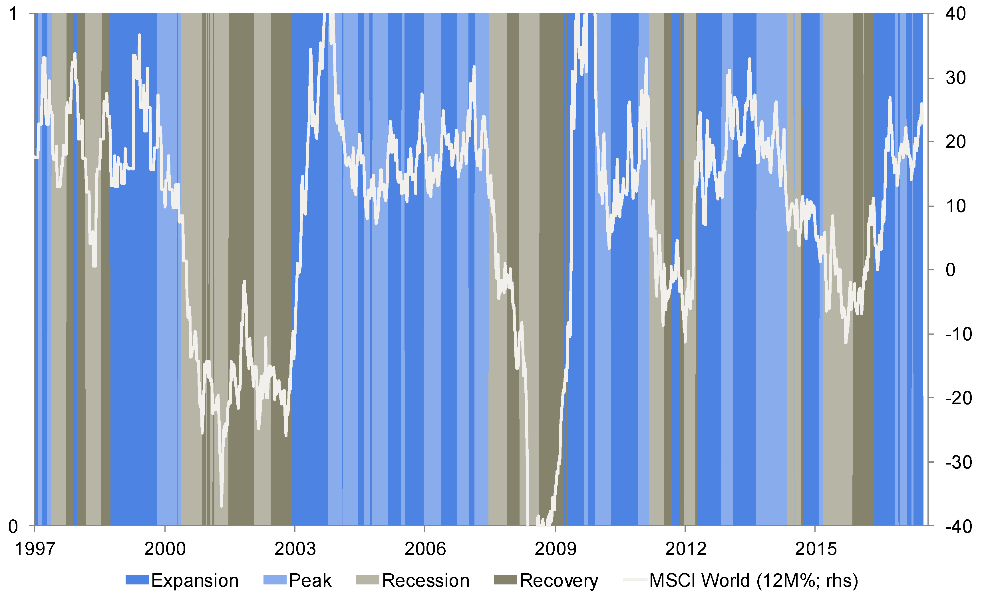
Figure 1 and Figure 2 present the business cycle indicators that were previously introduced. A value above 0 indicates that the market is in an uptrend (equities and corporate bonds are rising, as well as interest rates and commodities). In contrast, negative readings identify falling markets and increased risk aversion. The chart clearly emphasizes several risk-on periods (2003–2006, 2012–2014, 2016-today). Additionally, recessionary phases have been also identified at an early stage. The indicator points to further expansion ahead.
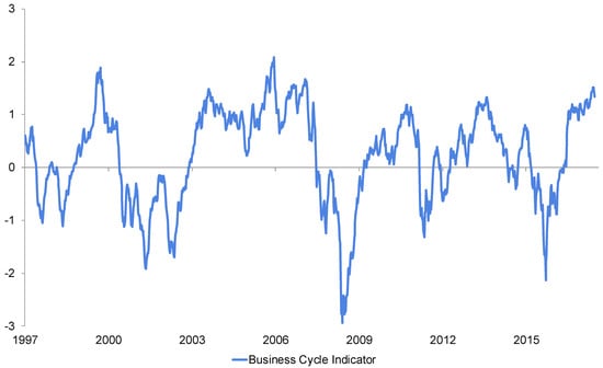
Figure 1.
(Global) business cycle indicator since 1995. Source: Authors’ own calculation.
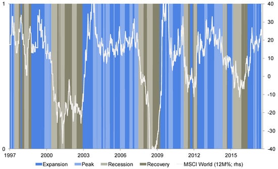
Figure 2.
Classification in business cycle phases and equity markets. Source: Authors’ own calculation.
To incorporate this indicator in our analysis framework, the conditional mean return concerning the business cycle was calculated over the entire sample to obtain a clear picture of the market dependency of individual risk premia. Table 3 summarizes these results.
Table 3.
Business cycle and risk premia returns.
The full range of risk premia strategies can be divided into two subgroups: cyclical strategies consisting of size and momentum which deliver superior returns in trending markets (in most cases uptrends) and defensive strategies such as quality and low volatility, which outperform when markets have peaked or show signs of entering a recession. The most striking observation is the relative independence of the value factor regarding market phases, as value is always placed at the center of the distribution (except for the peak phase which is marked by growth/momentum outperformance). One major reason for this behavior is its continuously changing composition of sectors. Phases have occurred where value has been more tilted to cyclical sectors such as consumer discretionary and financials as well as phases where value has mainly consisted of defensive stocks stemming from telecoms and/or utilities. These mentioned sectors usually show favorable valuation and/or high cost of equity.
Likewise, the conditional (annualized) volatilities of each strategy were calculated and ranked from risky via medium to conservative (Table 4).
Table 4.
Business cycle and risk premia volatilities.
It is also important to note the risk behavior of individual risk premia across different cycle regimes. Small caps show high volatility behavior, whereas low volatility stocks fluctuate least. Both observations coincide with our findings shown above. Momentum shows the typical behavior that was expected: high beta in uptrends and low beta in downtrends. We also note that value and carry stocks seem to be highly (positively) correlated with each other in turbulent phases. Both exhibit high volatility in recession/recovery phases, which points to increased cyclicality. Nevertheless, during expansion phases, value maintains its common features, whereas high dividend stocks show significantly fewer fluctuations. It seems that carry, in this case, behaves such as quality (during “good” economic times, high dividend payers coincide with stable dividend payers), which is also confirmed by their similar return characteristics. Table 5 presents the final results of the return behavior of individual risk premia across yield curve regimes.
Table 5.
Yield curve and risk premia returns.
This table emphasizes that size and momentum deliver superior returns in trending markets (in most cases uptrends, while defensive strategies such as quality and low volatility outperform when markets have peaked or might enter turbulent periods). However, as opposed to the business cycle analysis, momentum stocks perform poorly in recovery. This phase (as measured by the yield curve) is usually characterized by an extremely steep yield curve, which often coincides with a market low. As the trend direction changes quickly, momentum (which is low-beta at this time) is set to underperform. This finally results in the well-known momentum-crash (when looking at long-short portfolios). The performance ranking of different risk premia concerning the risk environment is shown in Table 6.
Table 6.
Risk environment and risk premia returns.
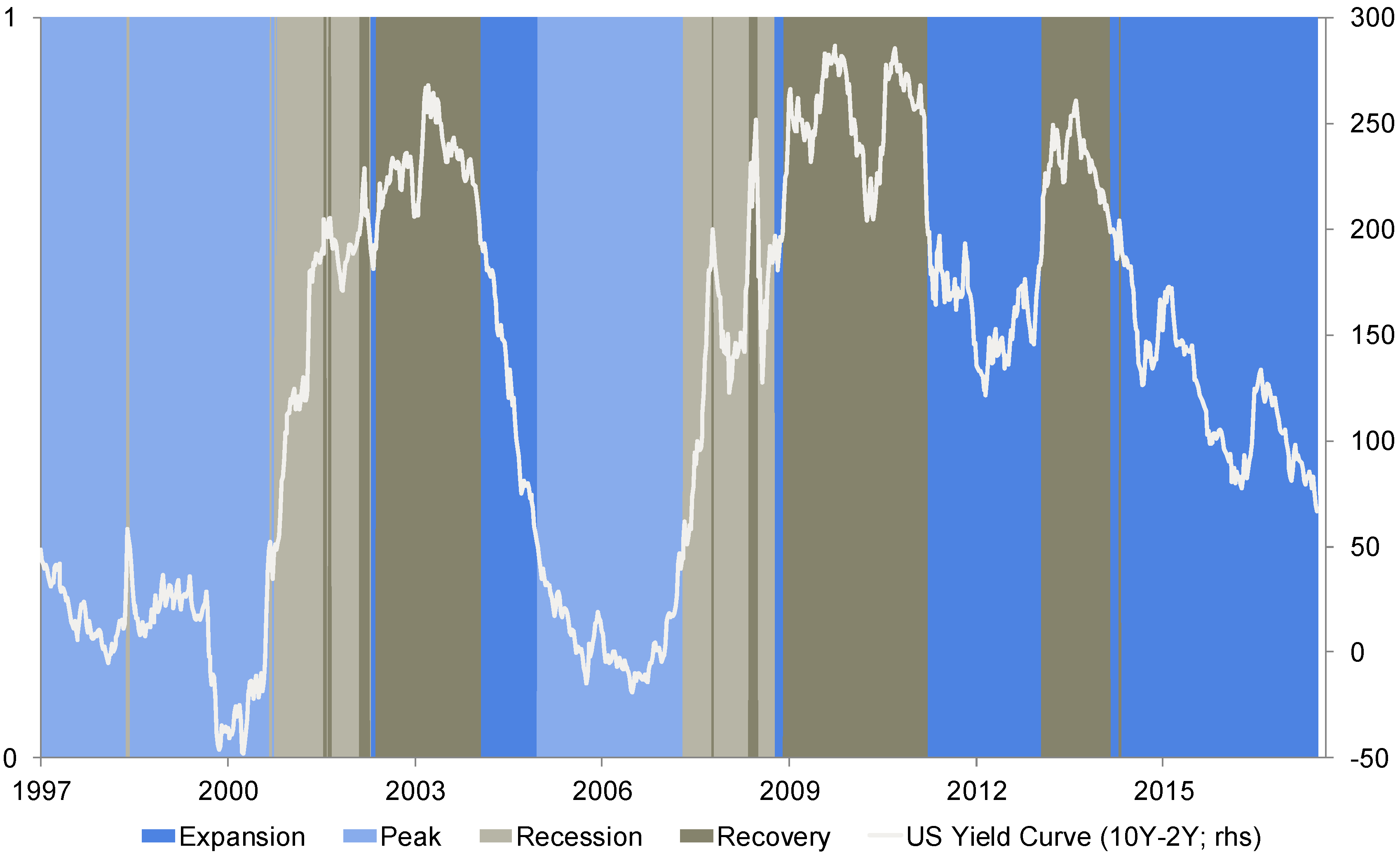
Here, the performance picture of individual risk premia seems to be rather heterogeneous as compared to the business cycle or yield curve strategy. Momentum continues to benefit in trending markets (complacency and risk on), while quality and low volatility stocks profit in risk-off phases. Small caps only show significant behavior at the tails of the risk distribution and carry returns are not assignable at all. Figure 3 presents the interest rate cycle as a function of the slope.
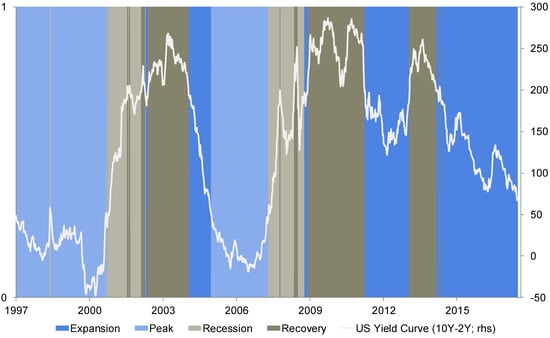
Figure 3.
Classification of the interest rate cycle and US yield curve. Source: Authors’ own calculation.
We now turn our attention to the results that are depicted in Table 7. Our business cycle strategy exhibits (except for the risk strategy) by far the most attractive return—risk-relation. It delivers both the highest return and alpha over the sample period. In contrast to the momentum strategy, which exhibits a high skewness in absolute terms, the business cycle strategy’s skewness is even lower than that of the (equal-weighted) factor index. The alpha reading of 0.04 seems to be relatively high and suggests a steady outperformance over time. The momentum and yield curves are not able to compete with this, but also show positive alpha values. The yield curve’s skewness (Table 6) of −0.98 is the lowest among all strategies; however, the return–risk ratio does not appear to be satisfactory. Nevertheless, it should be noted that the strategy based on the risk indicator delivers similar results (compared to the business cycle approach). In addition, skewness and alpha have the same magnitude, it refers that business cycle and risk perception are interlinked: economic expansion coincides with decreasing risk aversion, whereas economic downturns are associated with rising risk aversion. This is one of the main findings of this paper. It also confirms the behavior of the investors during the global financial crisis.
Table 7.
Factor Timing Strategies—Comparative Statistics.
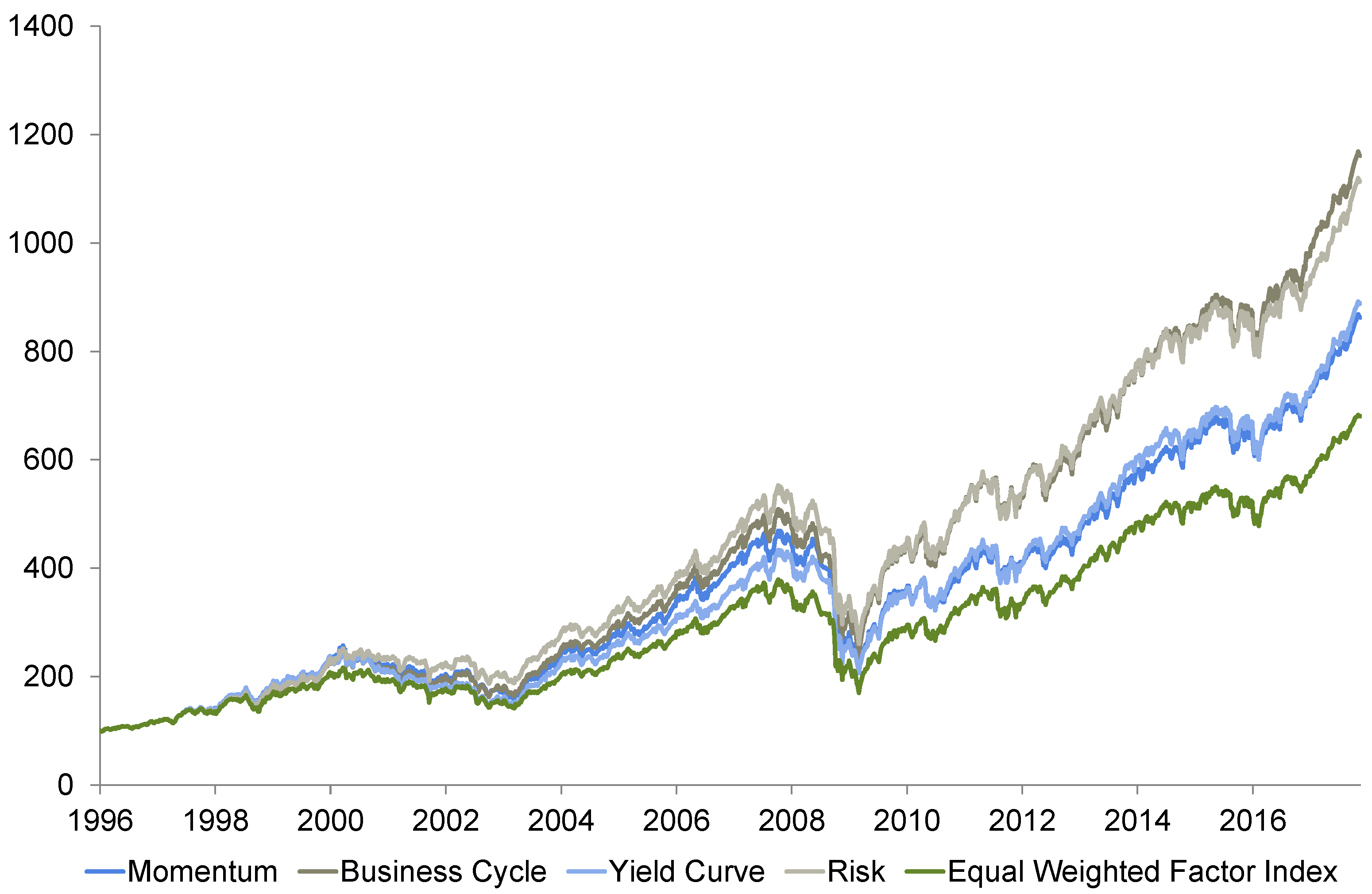
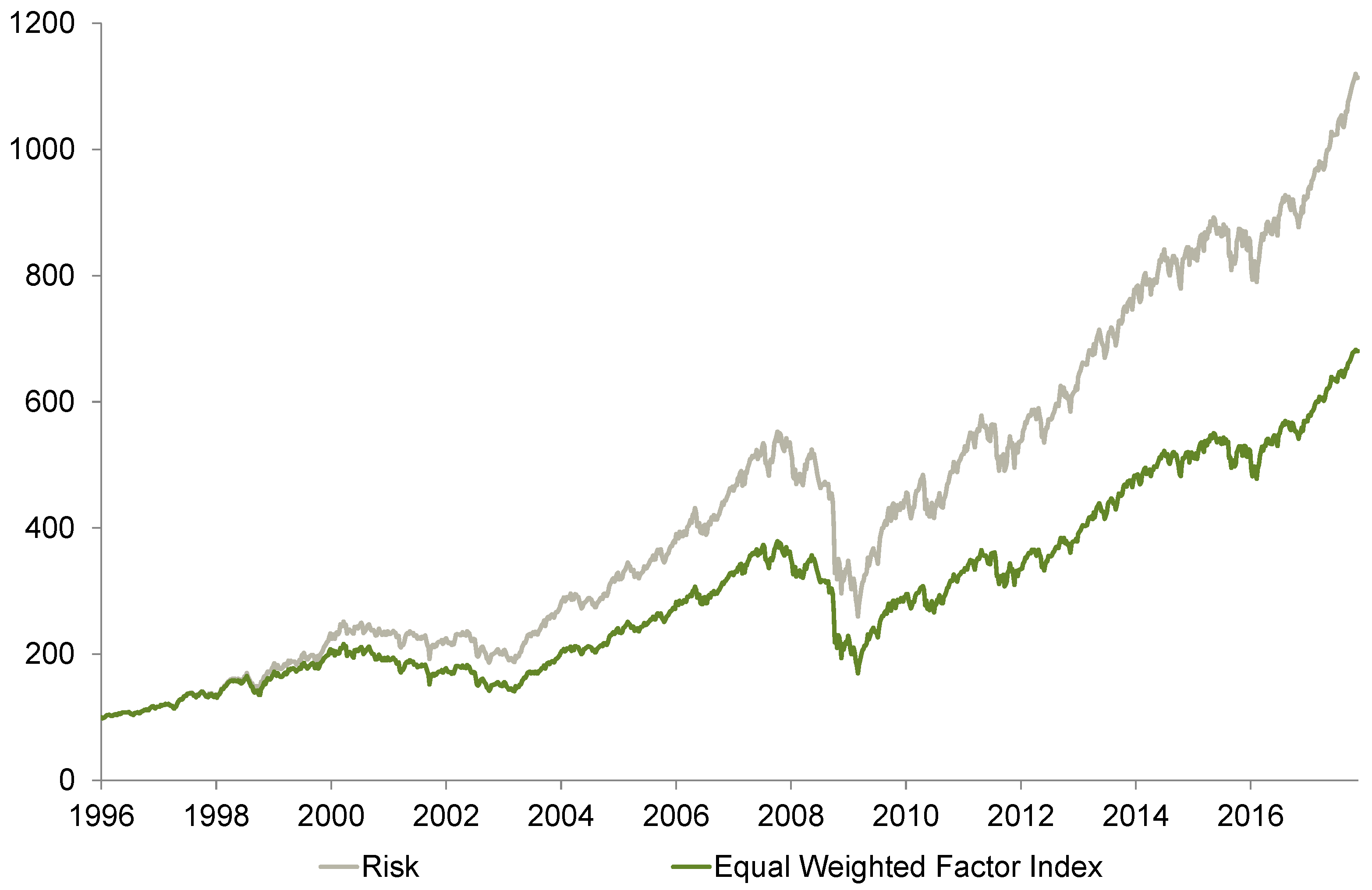
Thus, each strategy in Figure 4, Figure 5, Figure 6, Figure 7, Figure 8, Figure 9, Figure 10, Figure 11, Figure 12, Figure 13, Figure 14 and Figure 15 (business cycle, momentum, yield curve, and risk) outperforms the equal-weighted factor index. The business cycle strategy generates positive alpha. The excess beta of the business cycle strategy (above one most of the time) indicates that the strategy can successfully adapt to the current development of equity markets. Since equities are trending higher most of the time, the strategy anticipates this behavior by selecting factors with higher beta (which outperform in phases of rising stock markets) on average.
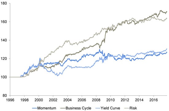
Figure 4.
The relative performance of factor timing strategies (benchmark: equal-weighted factor index). Source: Authors’ own calculation.
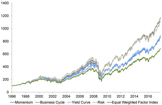
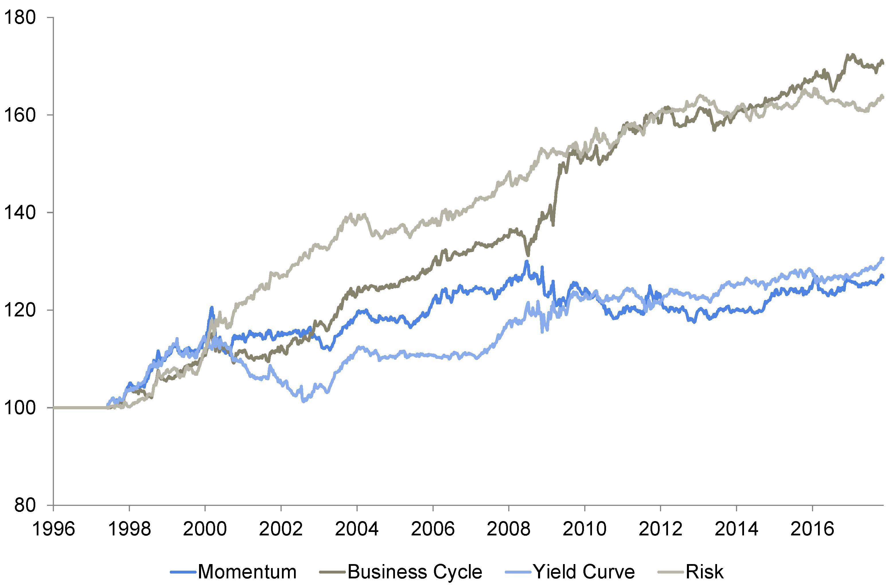
Figure 5.
Absolute performance of factor timing strategies. Source: Authors’ own calculation.
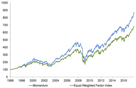
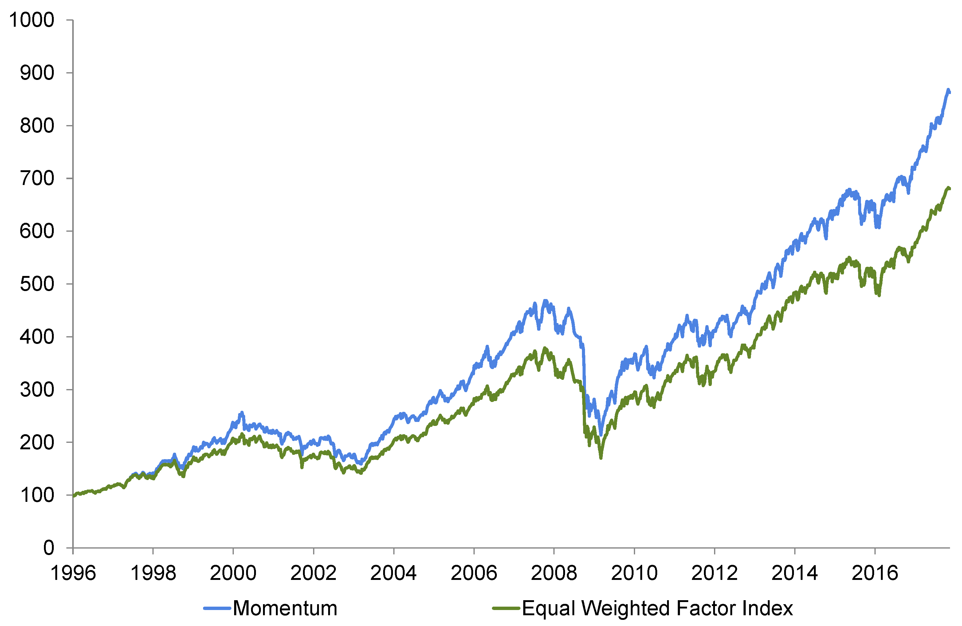
Figure 6.
Momentum strategy vs. equal-weighted factor index. Source: Authors’ own calculation.

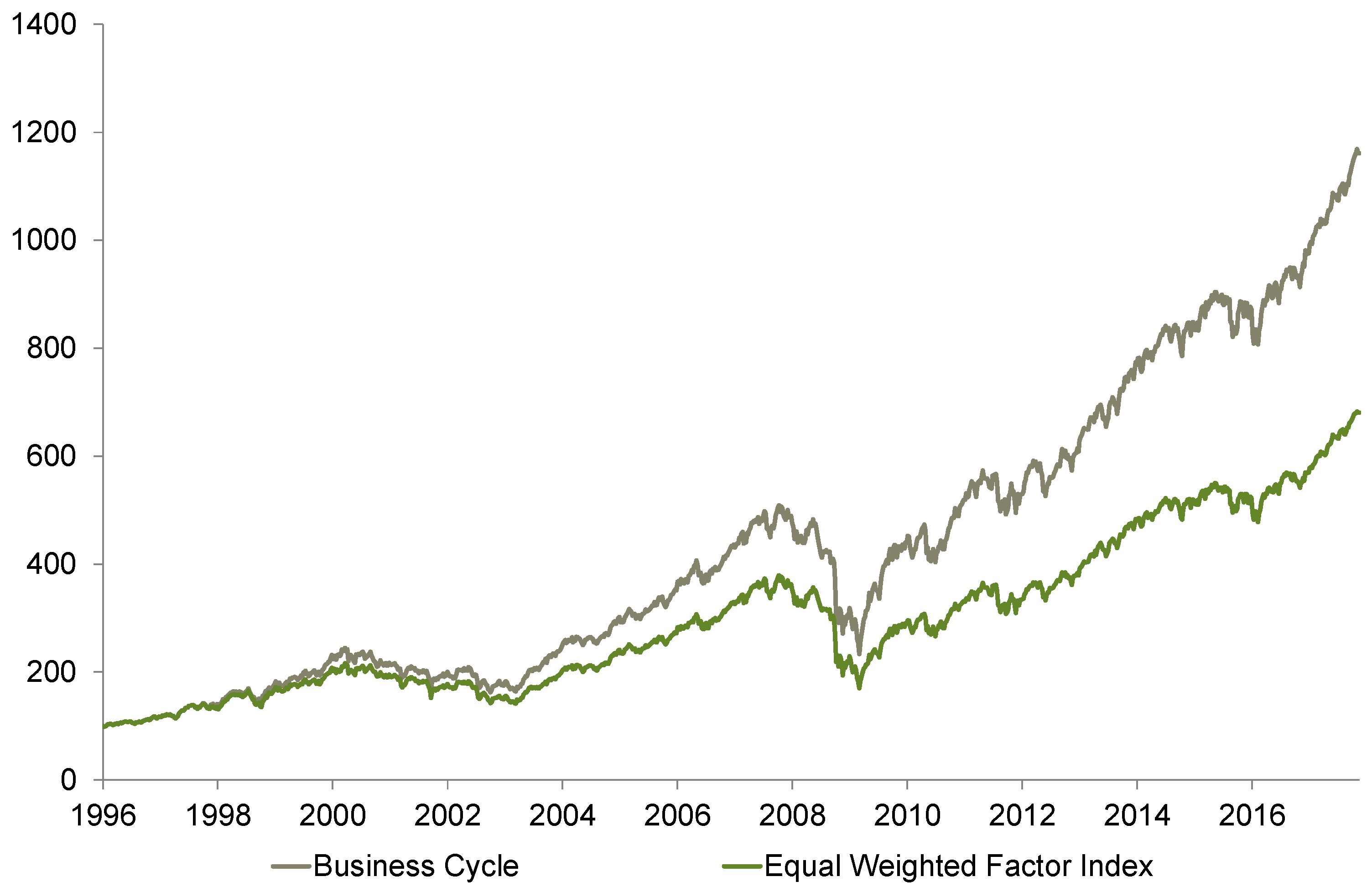
Figure 7.
Business cycle strategy vs. equal-weighted factor index. Source: Authors’ own calculation.
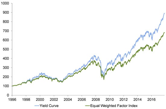
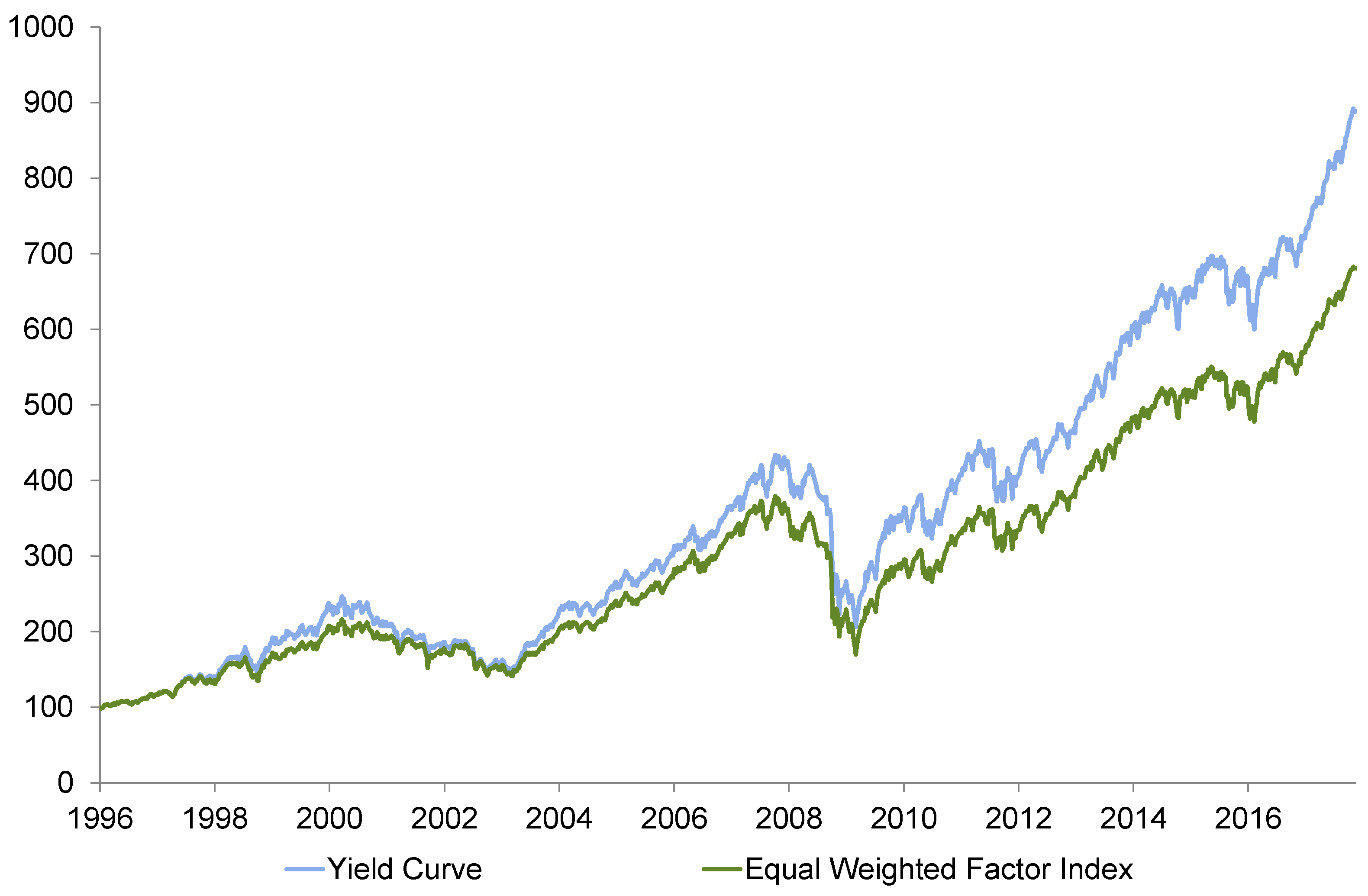
Figure 8.
Yield curve strategy vs. equal-weighted factor index. Source: Authors’ own calculation.
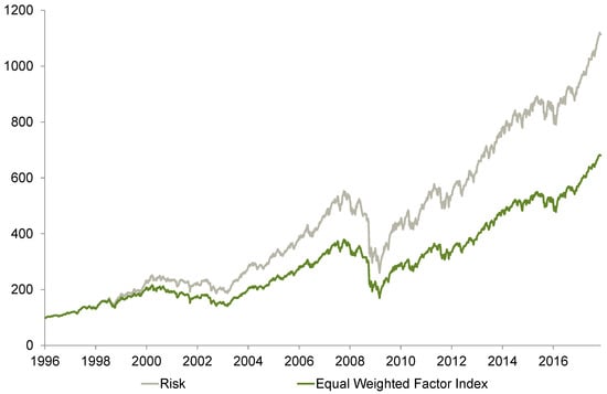
Figure 9.
Risk strategy vs. equal-weighted factor index. Source: Authors’ own calculation.
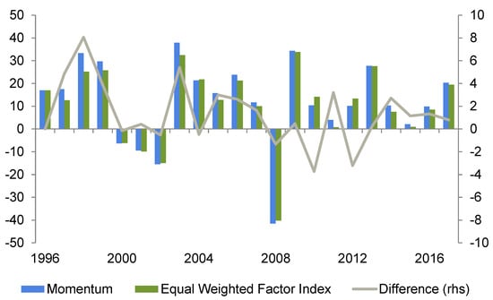
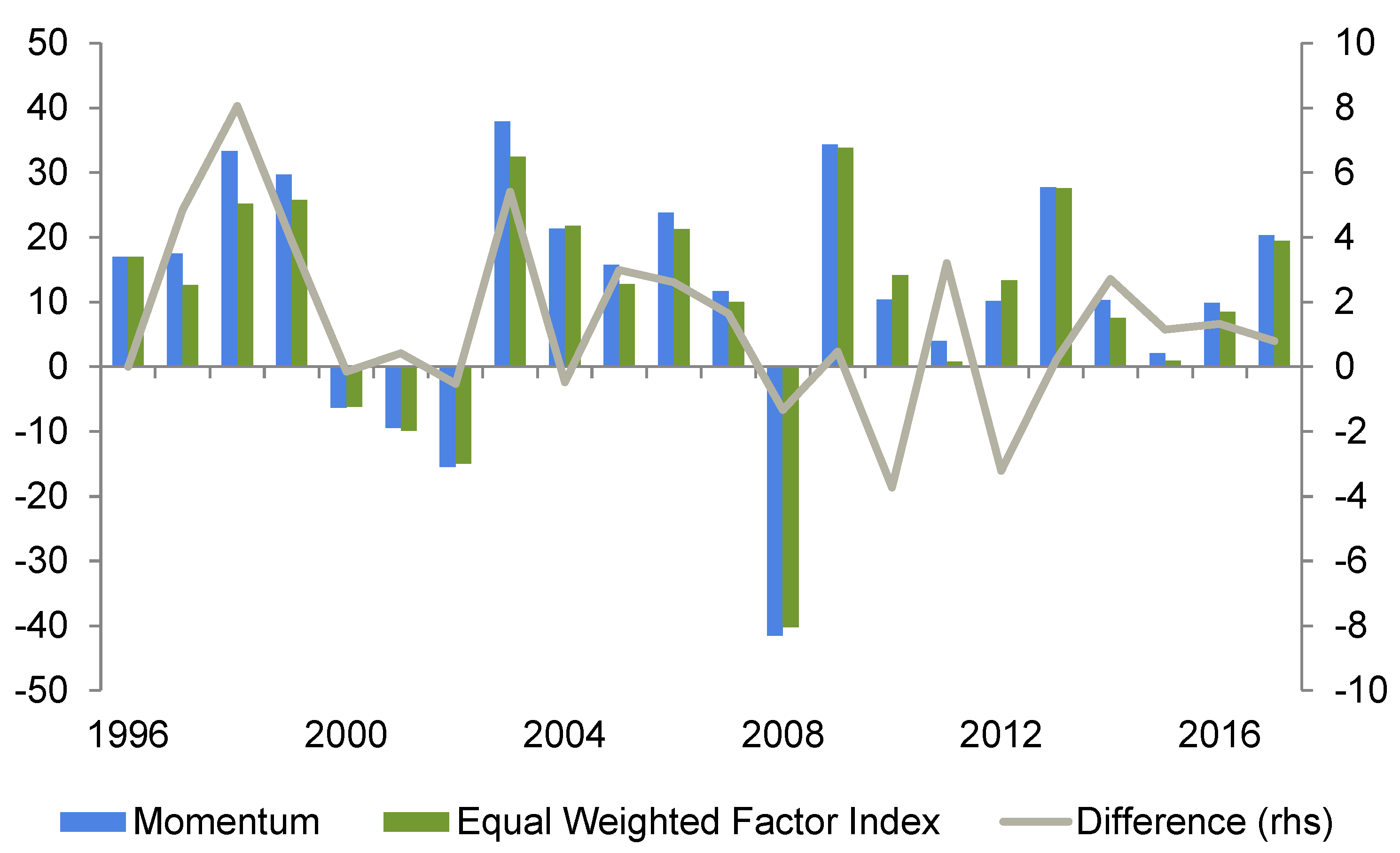
Figure 10.
Calendar year performance of momentum strategy. Source: Authors’ own calculation.
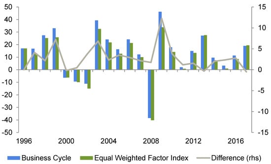
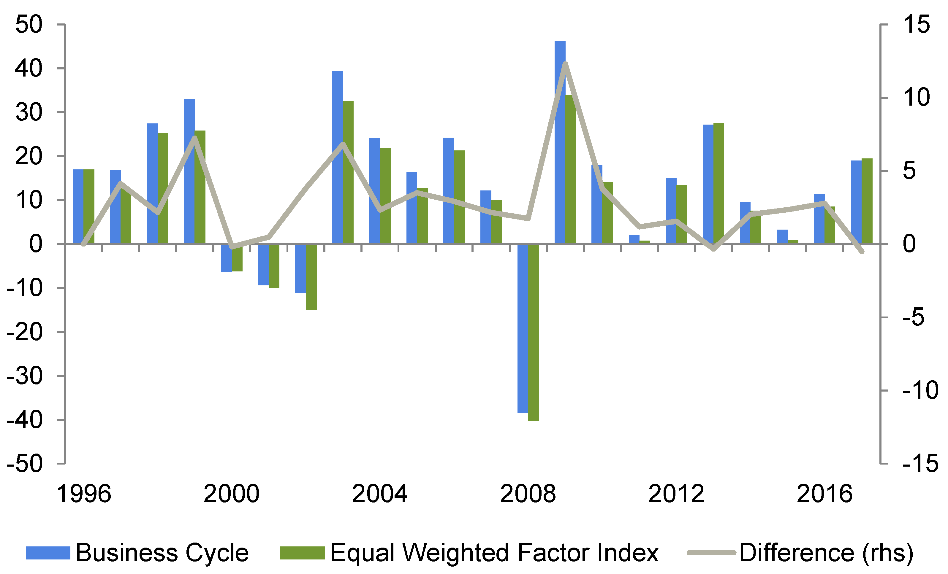
Figure 11.
Calendar year performance of business cycle strategy. Source: Authors’ own calculation.
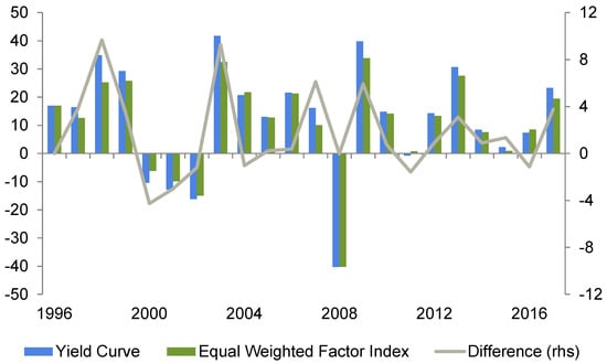
Figure 12.
Calendar year performance of yield curve strategy. Source: Authors’ own calculation.
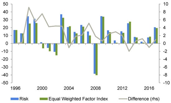
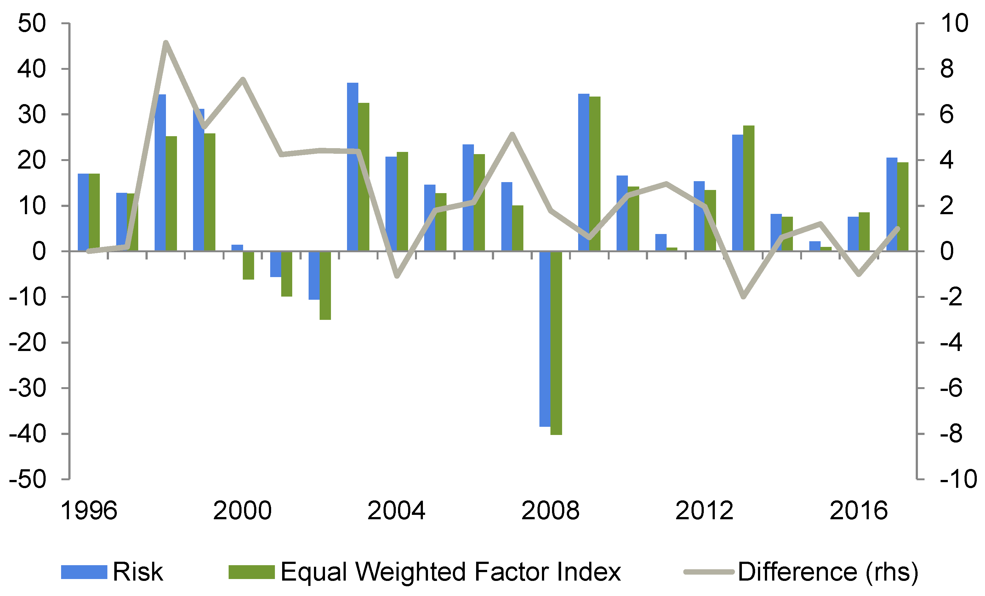
Figure 13.
Calendar year performance of risk strategy. Source: Authors’ own calculation.

Figure 14.
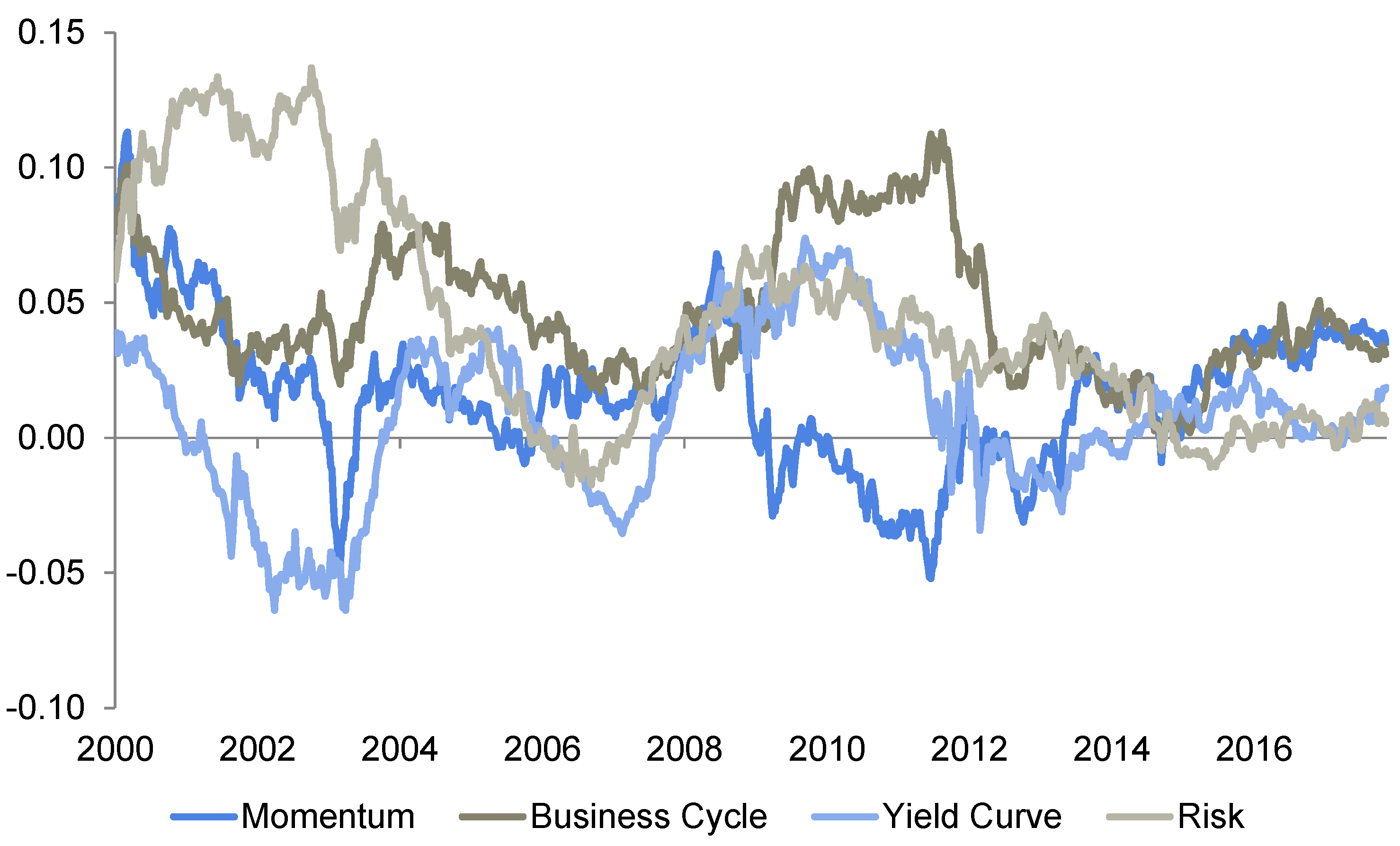
Three-year rolling alpha of risk premia timing strategies. Source: Authors’ own calculation.
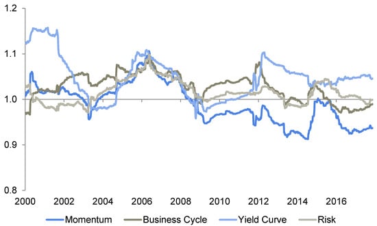
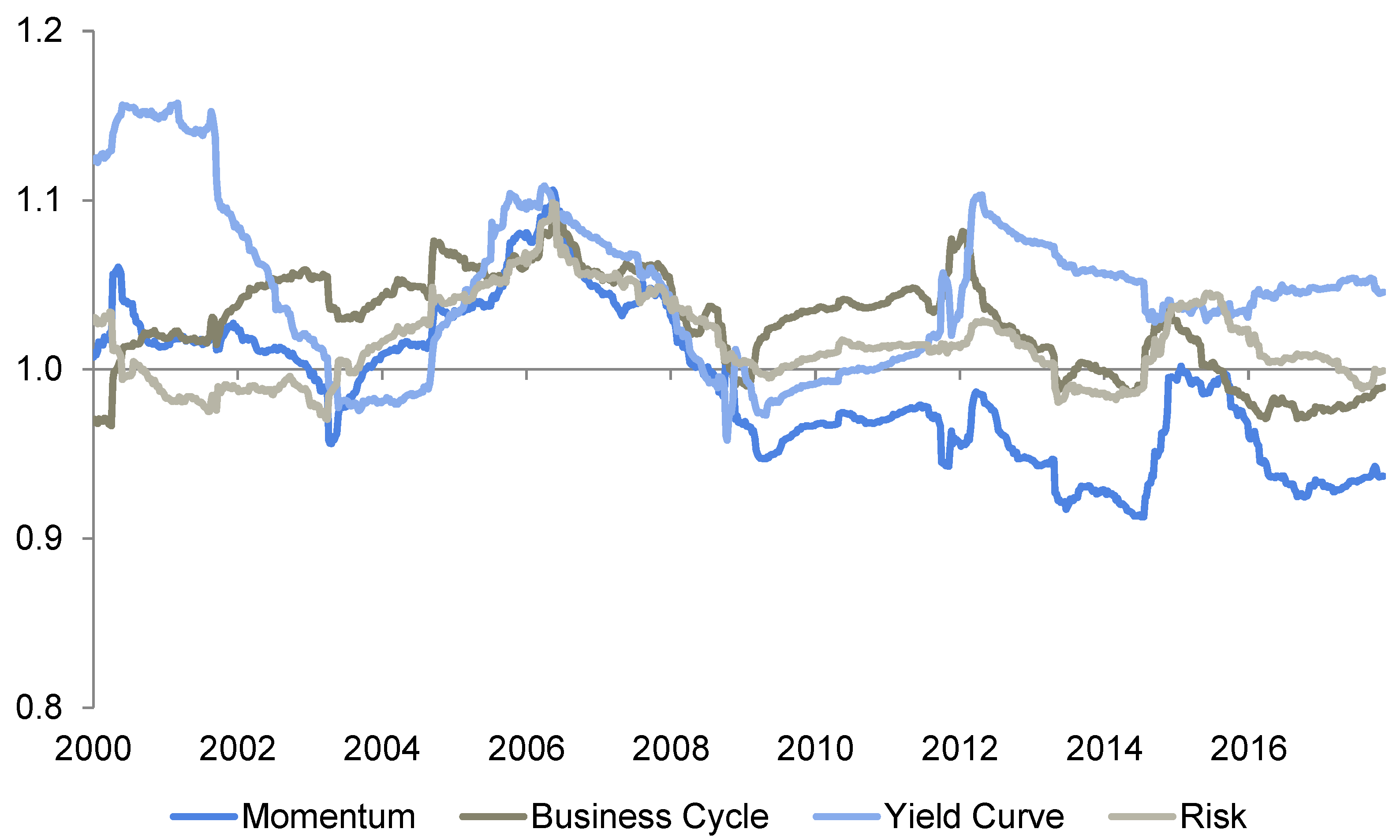
Figure 15.
The three-year rolling beta of risk premia timing strategies. Source: Authors’ own calculation.
5. Conclusions
The sample period is based on monthly data from January 1995 to September 2017. The universe consists of all stocks from the MSCI World index. This paper focuses on six risk premia strategies namely size, value, momentum, carry, quality, and low volatility. The risk and return characteristics of these risk premia have been investigated and factor timing strategies concerning the business cycle, interest rate cycle, and risk environment have been developed accordingly.
The robustness of these style allocation methods has been empirically examined by business cycles. In this regard, it was found that there is a close link between the business cycle and the prevalent risk regime, where economic expansion coincides with decreasing risk aversion and economic downturns lead to increased risk aversion. However, the business cycle strategy exhibits by far the most attractive return–risk relation. The excess beta of the business cycle strategy (greater than one most of the time) indicates that the strategy can successfully adapt to the current development of equity markets. Since equities are trending higher most of the time, the strategy anticipates this behavior by selecting factors with higher beta (which outperform in phases of rising stock markets) on average. It can be concluded that these models can predict future premia and therefore support the timing of certain factors. However, investors must be aware that indicators and models that may have worked in the past might not be accurate predictors for future returns.
The research of this paper is valuable to include extensions. First, the business cycle allocation scheme can be examined for further research and robustness. More precisely, it is the applied business cycle concurrent or ahead of the official business cycles as published by NBER (National Bureau of Economic Research), and how robust is the proposed business cycle model in the area of inflection points. Secondly, the combination of different factors should be examined in each case; the benefits of adding further risk factors such as ESG factors.
Author Contributions
Conceptualization, methodology, software, data curation—A.B.; validation, formal analysis, investigation, resources—A.Z.I.; validation, visualization, project administration—M.B. All authors have read and agreed to the published version of the manuscript.
Funding
This research is funded by LGT Bank AG.
Institutional Review Board Statement
Not applicable.
Informed Consent Statement
Not applicable.
Data Availability Statement
The data can be retrieved from Datastream and Bloomberg databases.
Acknowledgments
We wish to thank the Editor and the anonymous reviewers who helped us to improve our paper.
Conflicts of Interest
No conflicts of interest exist in this manuscript, and the manuscript is approved by all authors for publication. The work described was original research that has not been published previously and is not under consideration for publication elsewhere, in whole or in part. All the authors listed have approved the manuscript that is enclosed.
References
- Ahmerkamp, Jan, and James Grant. 2013. Optimal Carry and Momentum Returns in Futures Markets: A Compensation for Capital Constrained Hedge Funds? Available online: https://papers.ssrn.com/sol3/papers.cfm?abstract_id=2234458 (accessed on 14 May 2018).
- Ang, Andrew, Robert Hodrick, Yuhang Xing, and Xiaoyan Zhang. 2009. High Idiosyncratic Volatility and Low Returns: International and Further U.S. Evidence. Journal of Financial Economics 91: 1–23. [Google Scholar] [CrossRef] [Green Version]
- Arnott, Rob, Noah Beck, and Vitali Kalesnik. 2017. Forecasting Factor and Smart Beta Returns. Available online: https://www.researchaffiliates.com/documents/595-Forecasting-Factor-and-Smart-Beta-Returns.pdf (accessed on 14 June 2018).
- Asness, Clifford, Jacques Friedman, Robert Krail, and John Liew. 2000. Style timing: Value versus growth. Journal of Portfolio Management 26: 50–60. [Google Scholar] [CrossRef]
- Asness, Clifford, Tobias Moskowitz, and Lasse Heje Pedersen. 2013. Value and momentum everywhere. The Journal of Finance 68: 929–85. [Google Scholar] [CrossRef] [Green Version]
- Asness, Clifford, Andrea Frazzini, Robert Israel, and Tobias Moskowitz. 2015. Fact, fiction, and value investing. The Journal of Portfolio Management 42: 34–52. [Google Scholar] [CrossRef]
- Asness, Clifford, Swati Chandra, Antti Ilmanen, and Robert Israel. 2017. Contrarian factor timing is deceptively difficult. The Journal of Portfolio Management 43: 72–87. [Google Scholar] [CrossRef] [Green Version]
- Backhaus, Achim, and Aliya Zhakanova Isiksal. 2016. The impact of momentum factors on multi asset portfolio. Romanian Journal of Economic Forecasting 19: 146–69. [Google Scholar]
- Baker, Malcolm, Brendan Bradley, and Jeffrey Wurgler. 2011. Benchmarks as limits to arbitrage: Understanding the low volatility anomaly. Financial Analysts Journal 67: 40–54. [Google Scholar] [CrossRef] [Green Version]
- Bali, Turan, Robert Engle, and Scott Murray. 2016. Empirical Asset Pricing: The Cross Section of Stock Returns. Hoboken: John Wiley and Sons. [Google Scholar]
- Bansal, Ravi, and Amir Yaron. 2004. Risks for the long run: A potential resolution of asset pricing puzzles. The Journal of Finance 59: 1481–509. [Google Scholar] [CrossRef] [Green Version]
- Bansal, Ravi, Dana Kiku, Ivan Shaliastovich, and Amir Yaron. 2014. Volatility, the macroeconomy, and asset prices. Journal of Finance 69: 2471–511. [Google Scholar] [CrossRef] [Green Version]
- Banz, Rolf. 1981. The relationship between return and market value of common stock. Journal of Financial Economics 9: 3–18. [Google Scholar] [CrossRef] [Green Version]
- Barberis, Nicholas, and Robert Thaler. 2003. A survey of behavioral finance. In Handbook of the Economics of Finance, (1053–1128). Edited by G. M. Constantinides, M. Harris and R. M. Stulz. North Holland: Elsevier. [Google Scholar]
- Barberis, Nicholas, Andrei Shleifer, and Robert Vishny. 1998. A model of investor sentiment. Journal of Financial Economics 49: 307–43. [Google Scholar] [CrossRef]
- Basu, Sanjoy. 1977. Investment Performance of Common Stocks in Relation to the PriceEarnings Ratios: A Test of the Efficient Market Hypothesis. The Journal of Finance 32: 663–82. Available online: http://www.jstor.org/stable/2326304 (accessed on 1 December 2021). [CrossRef]
- Bender, Jennifer, Remy Briand, Dimitris Melas, and Raman Aylur Subramanian. 2013. Foundations of Factor Investing. Available online: https://www.msci.com/documents/1296102/1336482/Foundations_of_Factor_Investing.pdf/004e02ad-6f98–4730-90e0-ea14515ff3dc (accessed on 4 June 2021).
- Bender, Jennifer, Xiaole Sun, Ric Thomas, and Volodymyr Zdorovtsov. 2017. The Promises and Pitfalls of Factor Timing. Available online: https://jacobslevycenter.wharton.upenn.edu/wp-content/uploads/2017/09/Bender-Presentation.pdf (accessed on 5 June 2021).
- Binsbergen, Jules, Michael Brandt, and Ralph Koijen. 2012. On the timing and pricing of dividends. American Economic Review 102: 1596–618. [Google Scholar] [CrossRef] [Green Version]
- Bird, Ron, and Lorenzo Casavecchia. 2008. Conditional Style Rotation Model on Enhanced Value and Growth Portfolios: The European Experience, the Paul Woolley Centre @ UTS Working Paper Series 2. Available online: https://www.uts.edu.au/sites/default/files/wp2.pdf (accessed on 14 June 2018).
- Blitz, David, and Pim van Vliet. 2008. Global tactical cross-asset allocation: Applying value and momentum across asset classes. The Journal of Portfolio Management 35: 23–28. [Google Scholar] [CrossRef] [Green Version]
- Brunnermeier, Markus, Stefan Nagel, and Lasse Heje Pedersen. 2008. Carry trades and currency crashes. NBER Macroeconomics Annual 23: 313–48. [Google Scholar] [CrossRef] [Green Version]
- Campbell, John, and John Cochrane. 1999. By force of habit: A consumption-based explanation of aggregate stock market behavior. Journal of Political Economy 107: 205–51. [Google Scholar] [CrossRef]
- Carhart, Mark. 2012. On persistence in mutual funds findings of the empirical study. The Journal of Finance 52: 57–82. [Google Scholar] [CrossRef]
- Chan, Louis, Jason Karceski, and Josef Lakonishok. 1998. The risk and return from factors. Journal of Financial and Quantitative Analysis 33: 159–88. [Google Scholar] [CrossRef]
- Chan, Louis, Jason Karceski, and Josef Lakonishok. 1999. On portfolio optimization: Forecasting covariances and choosing the risk model. Review of Financial Studies 12: 937–74. [Google Scholar] [CrossRef]
- Clarke, Roger, Harindra De Silva, and Steven Thorley. 2006. Minimum-variance portfolios in the U.S. equity market. The Journal of Portfolio Management 33: 10–24. [Google Scholar] [CrossRef]
- Cochrane, John, and Monika Piazzesi. 2005. Bond risk premia. American Economic Review 95: 138–60. [Google Scholar] [CrossRef]
- Cowan, David, and Sam Wilderman. 2011. Rethinking Risk: What the Beta Puzzle Tells Us About Investing. GMO White Paper. [Google Scholar]
- Dai, Wei. 2017. Interest Rates and Equity Returns Paper. Available online: https://www.waldencapital.co.uk/uploads/files/When_Rates_Go_Up__Do_Stocks_Go_Down__(English).pdf (accessed on 14 June 2021).
- Daniel, Kent, and Tobias Moskowitz. 2013. Momentum Crashes. Swiss Finance Institute Research Paper 13: 61. Available online: https://ssrn.com/abstract=2371227 (accessed on 14 June 2021). [CrossRef]
- De Bondt, Werner, and Richard Thaler. 1985. Does the stock market overreact? The Journal of Finance 40: 793–805. [Google Scholar] [CrossRef]
- De Bondt, Werner, and Richard Thaler. 1987. Further evidence on investor overreaction and stock market seasonality. Journal of Finance 42: 557–81. [Google Scholar] [CrossRef]
- Dimson, Elroy, Paul Marsh, and Mike Staunton. 2016. Credit Suisse Global Investment Returns Sourcebook. Credit Suisse Research Institute. Available online: https://www.london.edu/faculty-and-research/academic-research/c/credit-suisse-global-investment-returns-sourcebook (accessed on 5 June 2021).
- Fama, Eugene, and Kenneth French. 1992. The cross-section of expected stock returns. The Journal of Finance 47: 427–65. [Google Scholar] [CrossRef]
- Frazzini, Andrea, and Lasse Heje Pedersen. 2014. Betting against beta. Journal of Financial Economics 111: 1–25. [Google Scholar] [CrossRef] [Green Version]
- Goldberg, Lisa, Ran Leshem, and Michael Branch. 2015. Factoring Profitability. In Risk-Based and Factor Investing. Edited by E. Jurczenko. Amsterdam: Elsevier, pp. 329–37. [Google Scholar]
- Graham, Benjamin. 1949. Intelligent Investor. New York: Harper and Brothers. [Google Scholar]
- Graham, Benjamin, and David Dodd. 1934. Security Analysis. New York: McGraw-Hill. [Google Scholar]
- Gügi, Patrick. 1996. Einsatz der Portfoliooptimierung im Asset Allocation-Prozess. Working Paper. Zürich: Zürich University. [Google Scholar]
- Harvey, Campbell. 1989. Time-varying conditional covariances in tests of asset pricing models. Journal of Financial Economics 24: 289–317. [Google Scholar] [CrossRef]
- Haugen, Robert, and Nardin Baker. 1991. The Efficient Market Inefficiency of Capitalization-Weighted Stock Portfolios. Journal of Portfolio Management 17: 35–40. [Google Scholar] [CrossRef]
- Hirshleifer, David. 2001. Investor Psychology and Asset Pricing. The Journal of Finance 56: 1533–97. [Google Scholar] [CrossRef] [Green Version]
- Hong, Harrison, and Jeremy Stein. 1999. A unified theory of underreaction, momentum trading, and overreaction in asset markets. The Journal of Finance 54: 2143–84. [Google Scholar] [CrossRef] [Green Version]
- Huji, Joop, and Marno Verbeek. 2009. On the use of multifactor models to evaluate mutual fund performance. Financial Management 38: 75–102. [Google Scholar] [CrossRef] [Green Version]
- Ilmanen, Antti. 2016. Smart investing in an environment of low expected returns. Journal of Investment Consulting 17: 4–12. [Google Scholar]
- Israel, Ronen, and Thomas Maloney. 2014. Understanding style premia. The Journal of Investing 23: 15–22. [Google Scholar] [CrossRef]
- Jagannathan, Ravi, and Tongshu Ma. 2003. Risk reduction in large portfolios: Why imposing the wrong constraints helps. The Journal of Finance 58: 1651–84. [Google Scholar] [CrossRef] [Green Version]
- Jegadeesh, Narasimhan. 1990. Evidence of predictable behaviour of security returns. The Journal of Finance 45: 881–98. [Google Scholar] [CrossRef]
- Jegadeesh, Narasimhan, and Sheridan Titman. 1993. Returns to buying winners and selling losers: Implications for stock market efficiency. The Journal of Finance 48: 65–91. [Google Scholar] [CrossRef]
- Jensen, Gerald, Jeffrey Mercer, and Robert Johnson. 1996. Business conditions, monetary policy, and expected security returns. Journal of Financial Economics 40: 213–37. [Google Scholar] [CrossRef]
- Koijen, Ralph, Hanno Lustig, and Stijn Van. 2017. The cross-section and time series of stock and bond returns. Journal of Monetary Economics 88: 50–69. [Google Scholar] [CrossRef] [Green Version]
- Lehmann, Bruce. 1990. Fads, martingales and market efficiency. Quarterly Journal of Economics 105: 1–28. [Google Scholar] [CrossRef]
- Leledakis, George, Ian Davidson, and Jeremy Smith. 2004. Does Firm Size Predict Stock Returns? Evidence from the London Stock Exchange. Available online: http://dx.doi.org/10.2139/ssrn.492283 (accessed on 4 June 2021).
- Lettau, Martin, Matteo Maggiori, and Michael Weber. 2014. Conditional risk premia in currency markets and other asset classes. Journal of Financial Economics 114: 197–225. [Google Scholar] [CrossRef] [Green Version]
- Lustig, Hanno, and Andrien Verdelhan. 2007. The cross section of foreign currency risk premia and consumption growth risk. American Economic Review 97: 89–117. [Google Scholar] [CrossRef] [Green Version]
- Moskowitz, Tobias, and Mark Grinblatt. 1999. Do industries explain momentum? The Journal of Finance 54: 1249–90. [Google Scholar] [CrossRef]
- Norges Bank. 2015. Financial Stability Report 2015. Available online: https://www.norges-bank.no (accessed on 4 June 2018).
- Ohlson, James. 1980. Financial ratios and the probabilistic prediction of bankruptcy. Journal of Accounting Research 18: 109–31. [Google Scholar] [CrossRef] [Green Version]
- Pastor, Lubos, and Robert Stambaugh. 2003. Liquidity Risk and Expected Stock Returns. Journal of Political Economy 111: 642–85. [Google Scholar] [CrossRef] [Green Version]
- Piotroski, Joseph. 2000. Value Investing: The use of historical financial statement information to separate winners from losers. Journal of Accounting Research 38: 1–41. [Google Scholar] [CrossRef] [Green Version]
- Roncalli, Thierry. 2017. A Primer on Alternative Risk Premia. Available online: http://www.thierry-roncalli.com/download/Alternative_Risk_Premia_WDWK.pdf (accessed on 5 June 2021).
- Schneeweis, Thomas, Garry Crowder, and Hossein Kazemi. 2010. The New Science of Asset Allocation: Risk Management in a Multi-Asset World. New Jersey: Wiley and Sons. [Google Scholar]
- Vayanos, Dimitri, and Paul Woolley. 2013. An institutional theory of momentum and reversal. The Review of Financial Studies 26: 1087–145. [Google Scholar] [CrossRef] [Green Version]
- Winkelmann, Kurt, Raghu Suryanarayanan, Ludger Hentschel, and Katalin Varga. 2013. Macro—Sensitive Portfolio Strategies: Pricing and Analyzing Macro Risk. Available online: https://www.msci.com/documents/10199/f8122b5d-eee4-4b67-b422-f4f2cc7f9b5c (accessed on 5 June 2021).
- Zhakanova Isiksal, Aliya Achim Backhaus, and Dennis Jung. 2019. Value investing across asset classes. Economic research-Ekonomska istraživanja 32: 1407–29. [Google Scholar] [CrossRef] [Green Version]
- Zhang, Lu. 2005. The value premium. The Journal of Finance 60: 67–103. [Google Scholar] [CrossRef]


Publisher’s Note: MDPI stays neutral with regard to jurisdictional claims in published maps and institutional affiliations. |
© 2022 by the authors. Licensee MDPI, Basel, Switzerland. This article is an open access article distributed under the terms and conditions of the Creative Commons Attribution (CC BY) license (https://creativecommons.org/licenses/by/4.0/).