Discretely Distributed Scheduled Jumps and Interest Rate Derivatives: Pricing in the Context of Central Bank Actions

Abstract

Interest rate dynamics are influenced by various economic factors, and central bank meetings play a crucial role concerning this subject matter. This study introduces a novel approach to modeling interest rates, focusing on the impact of central banks’ scheduled interventions and their implications for pricing bonds and path-dependent derivatives. We utilize a modified Skellam probability distribution to address the discrete nature of scheduled interest rate jumps and combine them with affine jump-diffusions (AJDs) in order to realistically represent interest rates. We name this class the AJD–Skellam models. Within this class, we provide closed-form formulas for the characteristic functions of a still broad class of interest rate models. The AJD–Skellam models are well-suited for using the interest rate version of the Fourier-cosine series (COS) method for fast and efficient interest rate derivative pricing. Our methodology incorporates this method. The results obtained in the paper demonstrate enhanced accuracy in capturing market behaviors and in pricing interest rate products compared to traditional diffusion models with random jumps. Furthermore, we highlight the applicability of the model to risk management and its potential for broader financial analysis.

1. Introduction

1.1. Motivation

The dynamics of interest rates in financial markets are influenced by a multitude of factors, ranging from economic indicators and market sentiment to governmental policies. Amidst this intricate web of influences, scheduled events orchestrated by central banks play a pivotal role in shaping interest rate movements (Kuncoro 2020). These events, such as the anticipated central bank meetings, have the potential to instantaneously impact interest rate targets, thereby triggering significant fluctuations in financial instruments.

During the intervals between central bank meetings, which typically last several weeks, the interest rate environment generally exhibits stability with the rates remaining constant. Figure 1 illustrates the trajectory of interest rate targets for the last five years in Brazil and the United States. This stability, observed in major economies, contributes to economic predictability, stabilizes macroeconomic growth rates, and contributes to financial development (Yang and Liu (2016) and Shaibu and Enofe (2021)). However, it also presents complexities concerning market anticipation, investor activities, and the need for central banks to communicate effectively and intervene in a timely manner (Kuncoro 2020). Maintaining unchanged interest rates between meetings is a crucial aspect of the broader monetary policy framework, which requires a delicate balance to promote economic growth, maintain price stability, and strengthen financial market resilience (da Silva and de Mello 2024). In conjunction with this, jumps in interest rates, occurring at predetermined dates, are the natural outcome of central bank meetings, and impact fully the pricing and hedging of complex interest rate derivatives. Such movements, therefore, deserve the utmost attention in modeling.

1.2. Related Literature

Traditional models often incorporate stochastic volatility, correlations, and random jumps to capture the inherent complexities of interest rate dynamics (Bouziane 2008). The literature suggests that jumps play a significant role in interest rate dynamics (Balduzzi et al. (2001), Glasserman and Kou (2003), and Lin et al. (2017)). However, they fail to accurately reflect the precise occurrence of scheduled events such as central bank announcements. These events, marked by predefined dates and specific adjustments in interest rates, deviate from the conventional random-jump framework.

Recognizing this limitation, recent studies have proposed ground-breaking approaches that introduce jumps with scheduled deterministic times into interest rate models. The use of Gaussian distribution for the size of scheduled jumps has been implemented in several studies, such as Heidari and Wu (2009), Kim and Wright (2014), Schloegl et al. (2023), and Fontana et al. (2024). By entering these deterministic jump times triggered by monetary authority meetings into the framework of interest rate models, the aim is to better encapsulate scheduled adjustments in interest rates triggered by central bank meetings. This departure from the traditional continuous-time and/or random jump structures offers a more realistic depiction of the market dynamics associated with these planned events.

No less important is the fact that, at these specific scheduled times, central bank interventions in interest rates are of a discrete nature; that is, they enforce discrete incremental movements to interest rates. Hence, they are ill-suited for modeling with Gaussian distributions or any distribution that imposes random movements in a continuous state space. Such distributions might inaccurately represent the discrete nature of central bank interventions. Piazzesi (2005) introduced a four-dimensional model that integrated the target rate as a scheduled jump process in a discrete state space. However, this model required the numerical solution of the Riccati equations in order to determine the solution for a pair of partial differential equations that separately addressed the time intervals with and without central bank meetings. The application of this model demonstrated its potential for providing valuable insights into the dynamic behavior of the target rate. In addition, Backwell and Hayes (2022) incorporated scheduled jumps in a discrete state space restricted to a five-jump possibility, symmetric around zero.

It is worth mentioning that instead of a sequence of jump times, Heidari and Wu (2009) used a one-jump assumption and relied on bootstrapping to circumvent this restriction. It is important to address the work of Genaro and Avellaneda (2018), where the focus remains on the Interbank Deposit Index (IDI) futures and options, for which there is a closed-form solution for the price of overnight rate products with a Gaussian structure and deterministic jump times. However, the results are limited to a one-factor diffusion Gaussian model and a finite set of possible outcomes in a central bank meeting with a nonparametric structure.

The following results are also noteworthy. Kim and Wright (2014) found that deterministic jump times in interest rate models can produce hump-shaped patterns in volatility and bond risk premiums, which is consistent with empirical findings. This finding suggests that scheduled central bank announcements can significantly influence bond markets, reinforcing the importance of modeling deterministic jump times. Johannes (2004) emphasizes that jumps play an important statistical role in continuous-time short-rate models, generating unexpected news about the macroeconomy. According to Johannes (2004), this aligns with the notion that deterministic jump times can be leveraged to better understand and predict market reactions to macroeconomic news. Glasserman and Kou (2003) discussed how jumps and diffusion risk premia enter the dynamics of simple forward rates, affecting implied volatilities in interest rate derivatives. This underscores the significance of incorporating jump risks into the models used for pricing and hedging interest rate derivatives (Glasserman and Kou 2003). Coffie (2023) studied the analytical properties of the true solution to the generalized delay Ait-Sahalia-type interest rate model with Poisson-driven jumps. It focuses on the finite-time strong convergence theory of the numerical solution under specific conditions, using new truncated Euler–Maruyama techniques.

1.3. Contribution

In this study, we eliminate the continuously distributed size and unexpected time problems by introducing the modified Skellam probability distribution without fixing the diffusion model, which aligns with the actual characteristics of central bank interventions. It presents a notable advancement in modeling scheduled jumps through its ability to simulate discrete movements of incremental changes, for instance of $0.25\%$, during central bank meetings, bringing, in this way, a higher level of fidelity to interest rate models and at the same time, preserving mathematical tractability.

Therefore, the introduction of scheduled deterministic jump times, in conjunction with the discrete modeling of jump sizes via the modified Skellam distribution, offers a more accurate representation of the impact of central bank policies on interest rates, significantly enhancing the accuracy of pricing bonds and interest rate derivatives. Accuracy is indeed sensitive here, because the presence of jumps in interest rates has a substantial impact on bond volatility and the prices of interest rate derivatives. For instance, Beber and Brandt (2009) note that increasing jump intensities and altering the distribution of jump sizes in interest rate models substantially affect the volatility of bond returns at all maturities. Jumps are also important for pricing interest rate options (Johannes 2004).

Incorporating scheduled jumps into interest rate models lies in the quest for increased accuracy in the pricing and hedging of complex interest rate derivatives. By refining the modeling approach to account for these shifts in interest rates due to scheduled events, there is an opportunity to enhance the precision of derivative pricing. This precision, achieved through the characteristic functions derived from these models, facilitates more accurate valuation and risk management of complex interest rate derivatives, such as the Interbank Deposit Index (IDI) options (see, e.g., Carreira and Brostowicz (2016) and Valentim (2022)), 30-Day Fed funds options (Genaro and Avellaneda 2018), and options on SOFR Futures (Xu 2021).

In summary, the introduction to the interest rate models of scheduled jumps with random sizes taking values in a discrete state space, governed by the modified Skellam distribution, aims to bridge the gap between theoretical modeling and the practical realities of financial markets. This novel approach not only enriches the modeling landscape but also offers a more comprehensive understanding of interest rate dynamics, enabling the process of decision-making in finance to be much more trustworthy.

This study focuses on computing the characteristic functions of a class of interest rate models, via which the prices of interest rate derivatives are obtained. We consider a broad class of processes to represent the interest rate over time, namely the so-called affine jump-diffusions (AJDs). As mentioned above, jumps occur at predetermined times with sizes that take values in the discrete state space and are governed by the modified Skellam distribution, thus preserving the essence of central bank determinations regarding interest rate targets.

The class of models developed here, named the AJD–Skellam model, can be viewed as a forward step in reference to Piazzesi (2005); Heidari and Wu (2009); Kim and Wright (2014); Backwell and Hayes (2022); Schloegl et al. (2023), and Fontana et al. (2024), as it presents the following novel features.

• We provide analytical solutions for the characteristic function of a still broad class of models within the AJD–Skellam class of interest rate models, enabling the fast pricing of bonds and derivatives depending on overnight interest rates;
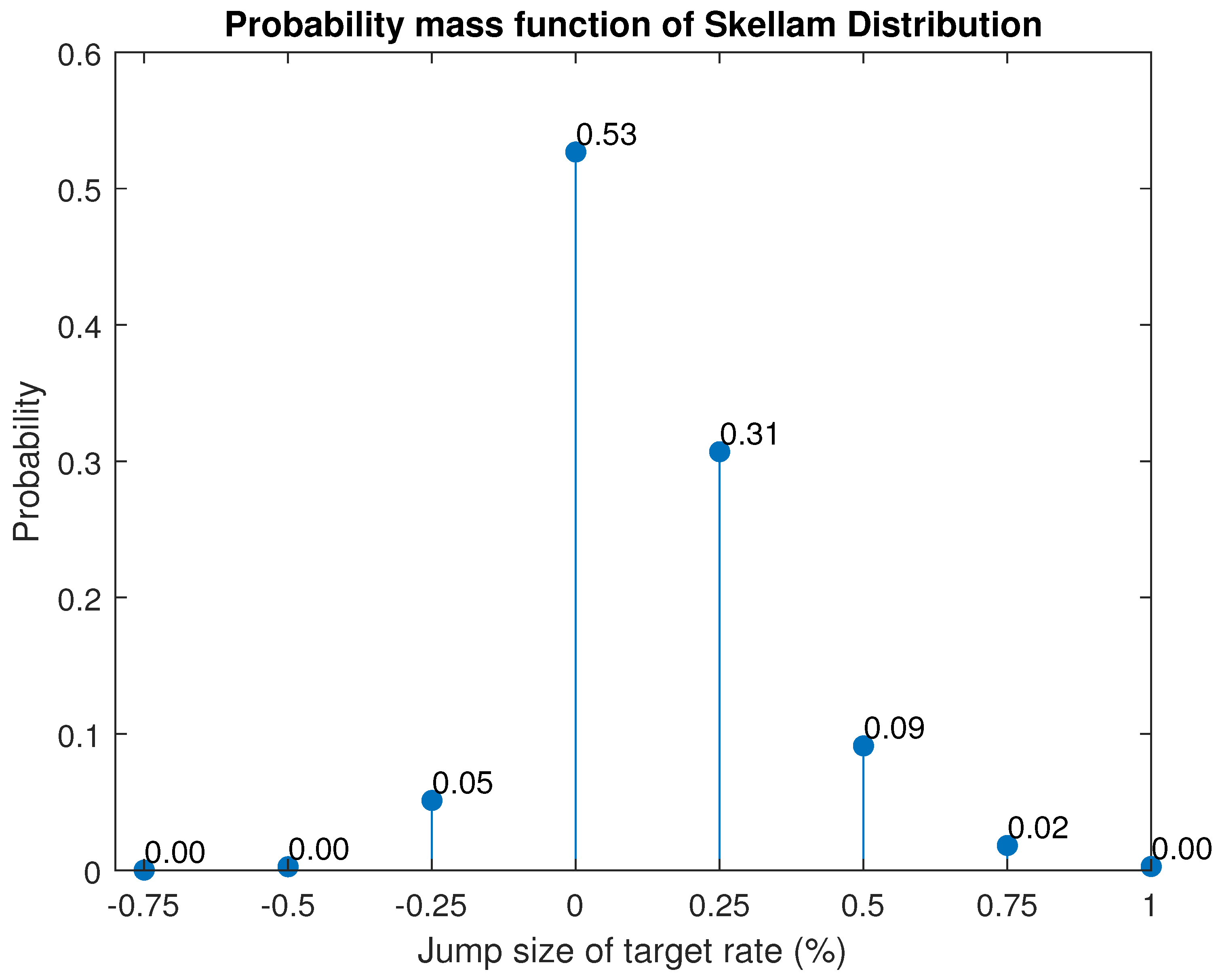
• Scheduled central bank announcements typically move the benchmark rate discretely in time and space. This class of models is consistent with this because the state space of the additive jump entry follows the modified Skellam probability distribution in discrete space. The usual distribution found in the literature for this purpose is Gaussian and, therefore, unrealistic. As far as the authors are aware, except for da Silva et al. (2023), the use of the Skellam distribution or its modifications do not exist in the context of pricing derivatives in financial markets. da Silva et al. (2023) obtained the price of an interest rate derivative of a recent vintage introduced in the Brazilian financial market, namely, the COPOM option (the acronym stands for Monetary Policy Committee);
• The model can easily allow jumps with stochastic volatility, correlations between Brownian motions, and additional random jump times. A closed-form formula exists even if the Vasicek (AJD) model is enhanced, as shown below;
• The exponential affine format of the resulting characteristic function allows us to calculate, numerically at least, via the celebrated Fourier-cosine series (COS) method (see Oosterlee and Grzelak 2019), the price of complex interest rate derivatives, and not bond prices only.
  Remark: The use of the COS method was confined to stock markets until recently, when da Silva et al. (2019) and da Silva et al. (2020) adapted its use to interest rate markets. A key point that permitted the authors to adapt the COS method to the needs of pricing derivatives in interest rate markets was determining that the integral of the interest rate process—and not the interest process per se—was an adequate mathematical object to achieve the pricing results. Hence, this is a supplementary contribution to this study.

1.4. Paper Outline

The remainder of this paper is organized as follows. Section 2 presents the methodology used in this study. Section 2.1 introduces the modified Skellam distribution and exhibits the exponential format of the associated characteristic function. Benefiting from this exponential format, we can derive closed-form expressions of the characteristic function associated with the integrated interest rate process, under the requirement of scheduled deterministic times for the jump rate and Skellam-shaped jump sizes. By the integrated interest rate process, we refer to the integral of the affine jump-diffusion representing the interest rates over time. In Section 2.2, the COS method is recovered. Section 3 provides the following results.

• We present the class of AJD–Skellam models, which connect the interest rate diffusion process with scheduled, discretely distributed jumps;
• The closed-form formula for the characteristic function of one and two-factor models, with both constant and time-dependent Skellam parameters, is provided. The particular case where the diffusion process is given by the Vasicek model is also shown;
• We apply the COS method, through which we calculate the probability density functions associated with the integrated interest rate processes and, ultimately, the derivative prices. Inter alia, the Vasicek model with and without Skellam jumps was addressed, while prices referring to the (zero-coupon) bonds and the IDI call option are shown;
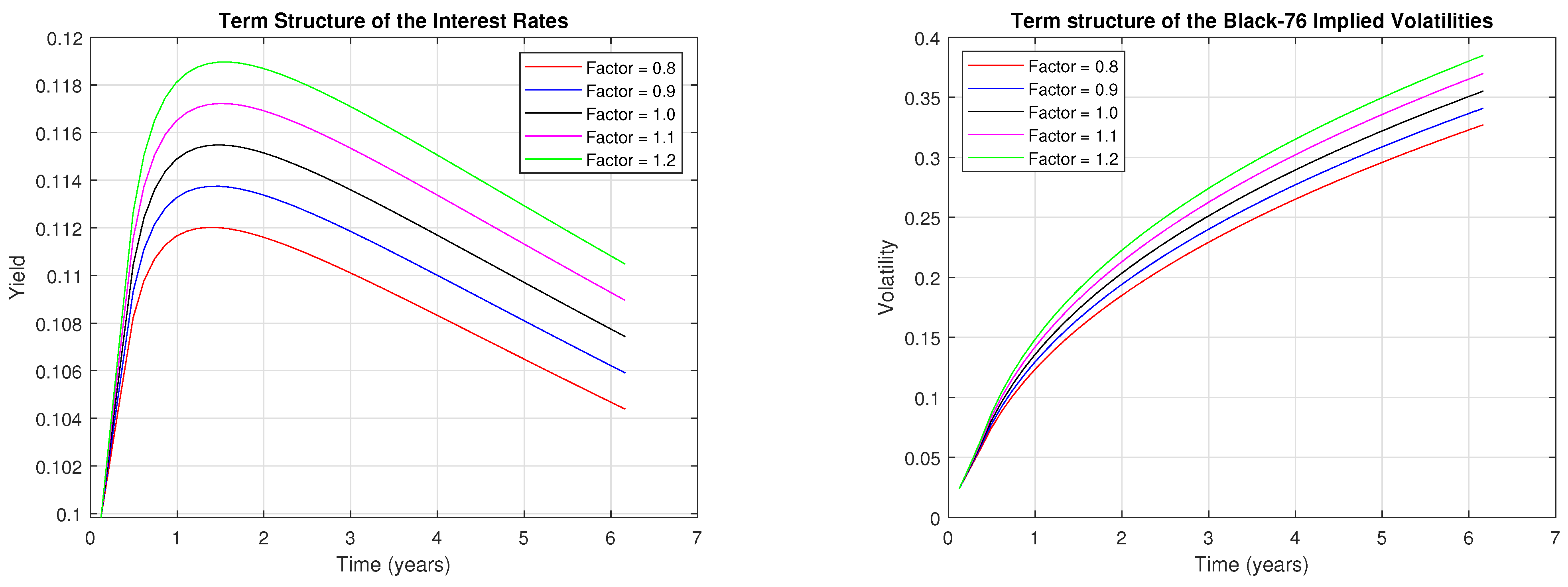
• We exhibit the term structure of interest rates under the Vasicek model equipped with Skellam jumps with time-varying parameters, as well as the Black-76 Implied Volatilities;
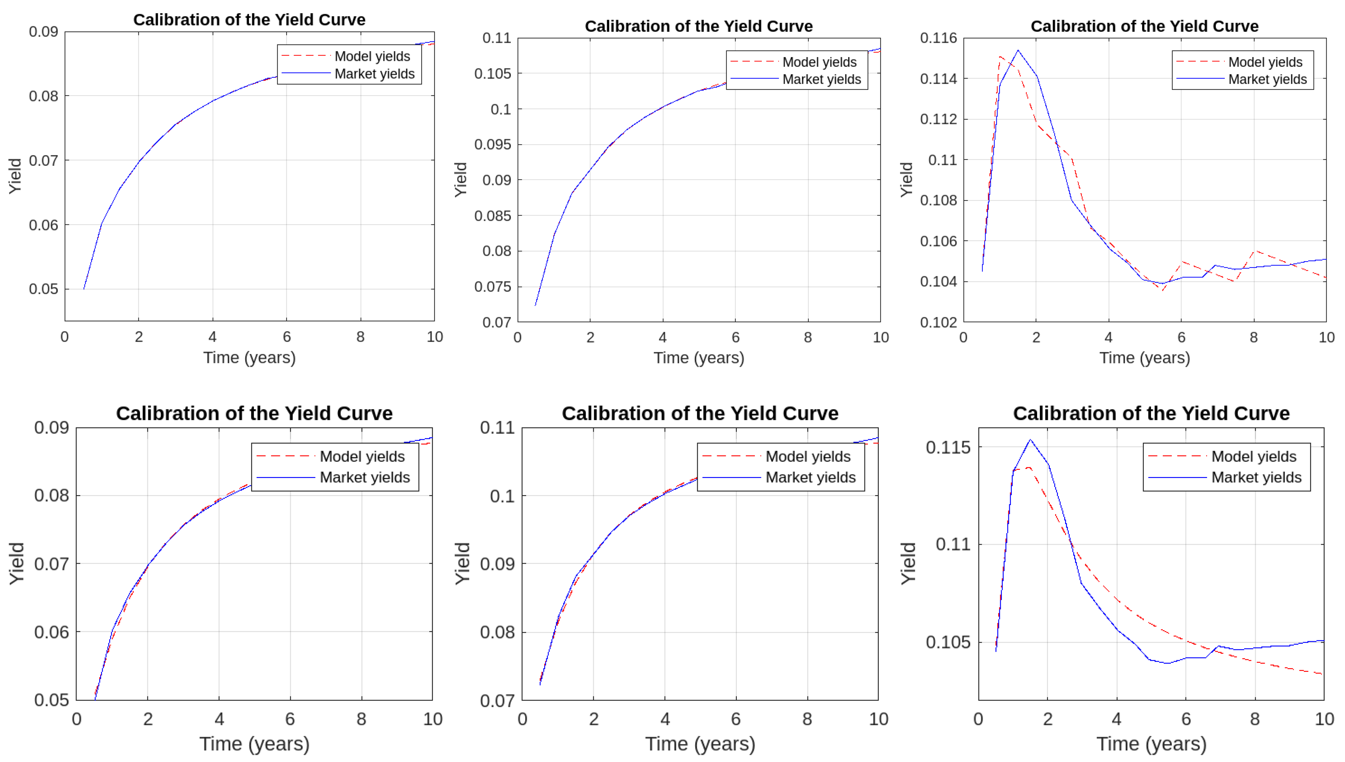
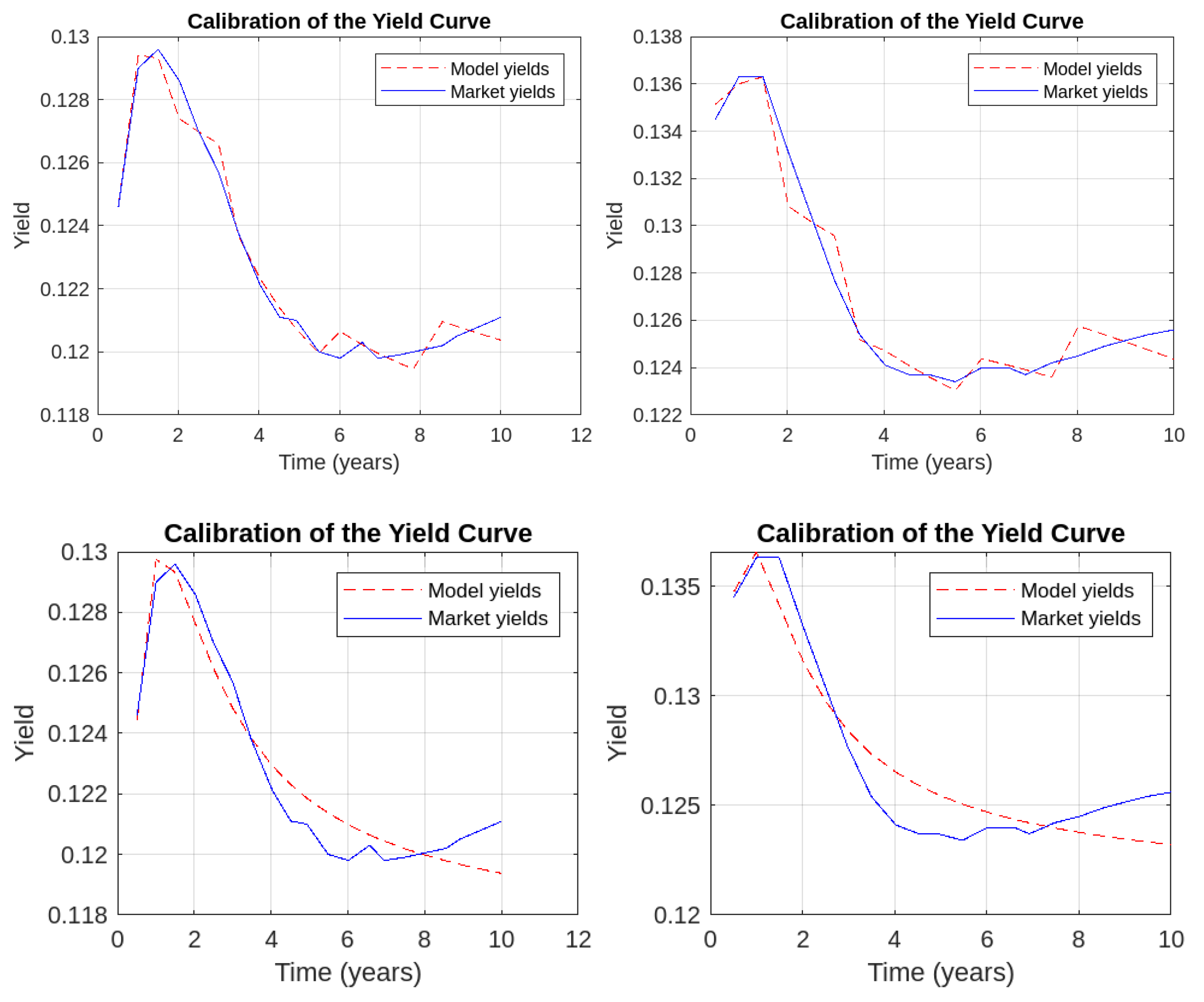
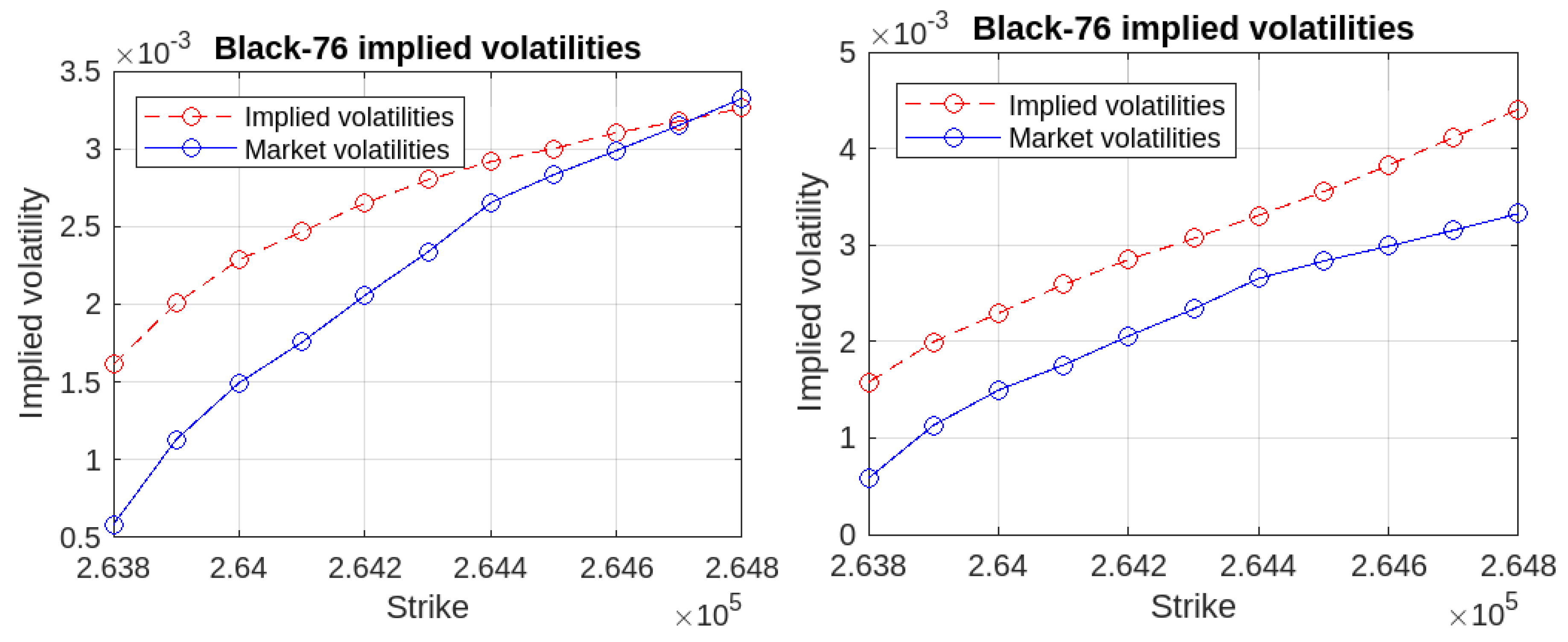
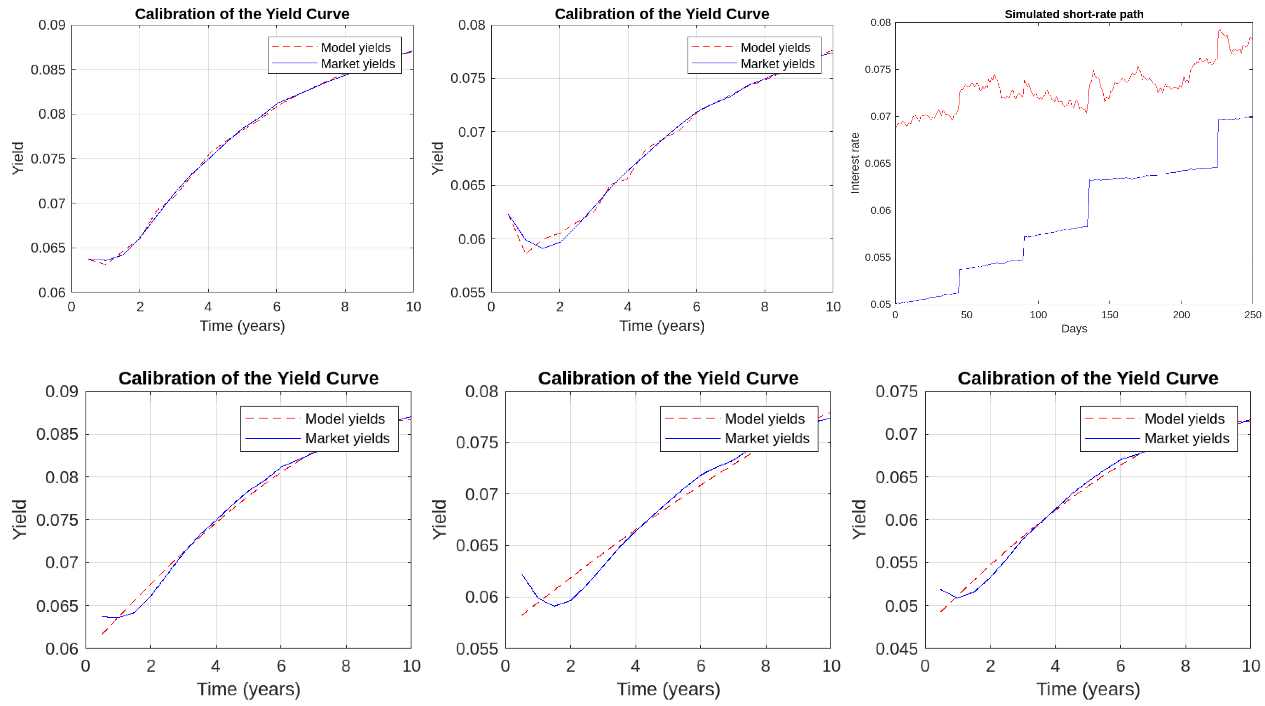
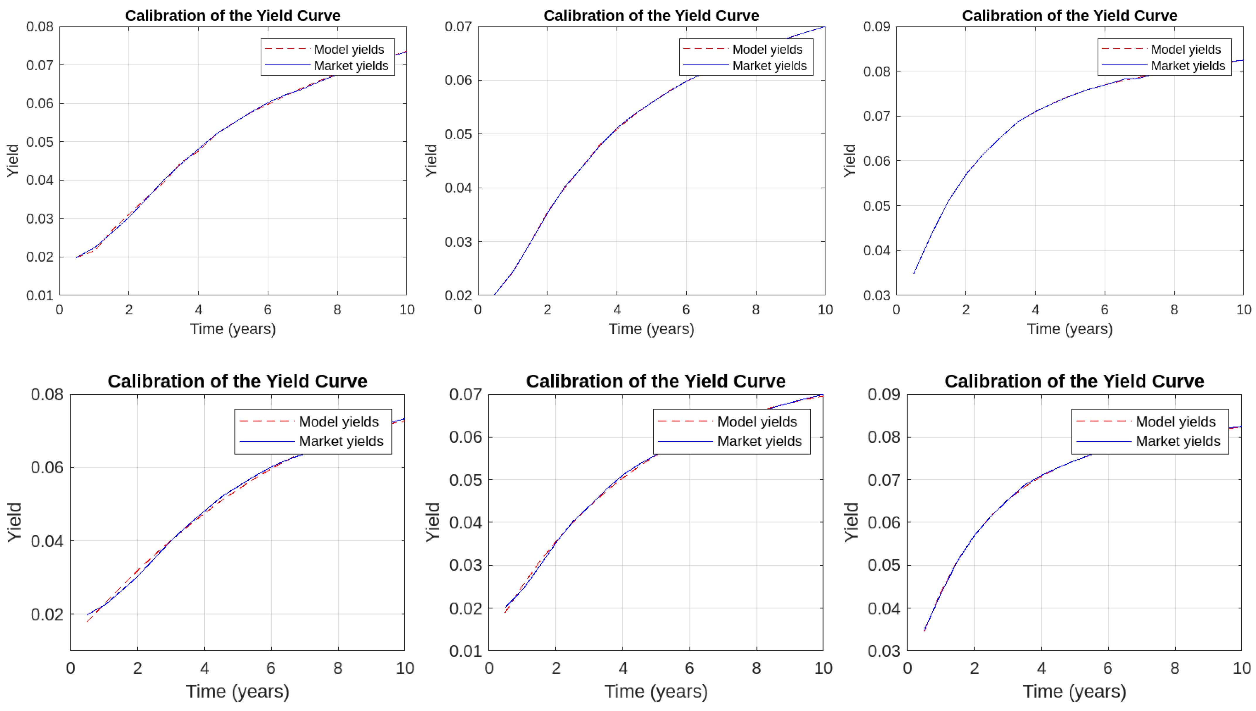
• We show a specific model calibration of term structure of the interest rates and the IDI option implied volatilities. We compared the performance with that of an interest rate model governed by Gaussian jumps;
• Interpretation of the model’s parameters is highlighted.

Section 4 discusses the results and Section 5 concludes the study.

2. Methodology

This section provides some theoretical underpinnings available in the existing literature, which we use to model interest rates and calculate financial derivative contracts. We introduce the probability distribution used to model the size of interest rate jumps following monetary policy decisions and explain the COS method for option pricing. By deriving the characteristic function of our model class in the Results section, we set the stage for accurate derivative pricing, highlighting the novel integration of discrete scheduled jumps within the affine jump-diffusion framework.

2.1. The Skellam Model for Jumps

The Skellam distribution arises as the discrete probability distribution of the difference between two statistically independent random variables $N_1$ and $N_2$, each Poisson distributed with mean values ${\mu }_1$ and ${\mu }_2$, respectively (Johnson et al. 2006). This supports on $\{\dots ,-2,-1,0,1,2,\dots \}$ and the mass probability function is given by

$$p(k;{\mu }_1,{\mu }_2)=\mathbb{P}\{N_1-N_2=k\}=e^{-({\mu }_1+{\mu }_2)}{\left(\frac{{\mu }_1}{{\mu }_2}\right)}^{k/2}{I}_k\left(2\sqrt{{\mu }_1{\mu }_2}\right),$$

(1)

where $I_k(·)$ is the modified Bessel function of the first kind, namely,

$$I_k\left(z\right)={\left(\frac{z}{2}\right)}^k\sum _{i=0}^{\infty }\frac{{\left(\frac{z^2}{4}\right)}^i}{i!\Gamma (k+i+1)},$$

(2)

with

$$\Gamma \left(v\right)=\underset{0}{\overset{\infty }{\int }}{s}^{v-1}{e}^{-s}ds.$$

(3)

The characteristic function of a random variable X with the Skellam distribution is given by

$${\widehat{f}}_X(u;{\mu }_1,{\mu }_2)=\mathbb{E}\left[e^{iuX}\right]=e^{-({\mu }_1+{\mu }_2)+{\mu }_1{e}^{iu}+{\mu }_2{e}^{-iu}}$$

(4)

Hence, a random variable X that induces the Skellam distribution has two desirable qualities: (i) its (Skellam) distribution is discrete, and (ii) its characteristic function has an exponential format.

da Silva et al. (2023) recently introduced the modified Skellam distribution, which is the distribution of $Y=cX+d$, where X is a random variable equipped with the Skellam distribution. Clearly, the domain of Y is

$$\{\dots ,-2c+d,-c+d,d,c+d,2c+d,\dots \}.$$

Therefore, Y is no longer a Skellam type, except for $c=1$ and $d=0$. For instance, it is easy to see that $c=\frac{1}{400}$ and $d=0$ imply the following domain.

$$\{\dots ,-0.50\%,-0.25\%,0,0.25\%,0.50\%,\dots \}.$$

We have that the characteristic function of Y is given by

$$\begin{array}{ccc}\hfill {\widehat{f}}_Y\left(u\right)& =& \mathbb{E}\left[e^{iuY}\right]=e^{idu}\mathbb{E}\left[e^{icuX}\right]\hfill \\ \hfill & =& e^{idu}{\widehat{f}}_X\left(cu\right)=e^{-({\mu }_1+{\mu }_2)+idu+{\mu }_1{e}^{icu}+{\mu }_2{e}^{-icu}}\hfill \end{array}$$

(5)

where, to avoid notational burden, we write ${\widehat{f}}_{·}\left(u\right)$ instead of ${\widehat{f}}_{·}(u;{\mu }_1,{\mu }_2)$. Therefore, the modified Skellam distribution is still discrete and the associated characteristic functions are still in an exponential format.

For later use, we have that

$$\begin{array}{ccc}\hfill M_Y\left(t\right)& =& \mathbb{E}\left[e^{tY}\right]=e^{dt}\mathbb{E}\left[e^{ctX}\right]\hfill \\ \hfill & =& e^{dt}{M}_X\left(ct\right)=e^{-({\mu }_1+{\mu }_2)+dt+{\mu }_1{e}^{ct}+{\mu }_2{e}^{-ct}}\hfill \end{array}$$

(6)

where $M_{·}$ denotes the moment generating functions.

Figure 2 shows an example of the probability mass function of the modified Skellam distribution with parameters $({\mu }_1,{\mu }_2)=(0.6,0.1)$ and, $c=\frac{1}{400}$ and $d=0$.

2.2. The COS Method: Representing Continuous Random Variables and Derivatives Prices via Fourier-Cosine Series

In the domain of derivative pricing, several numerical methods have been explored in the literature. These include the finite difference method, finite element method, Fast Fourier Transform (FFT), and Monte Carlo, each offering unique approaches to valuation challenges (see, for instance, Wilmott (2006) for finite differences, Topper (2005) for finite elements, Carr and Madan (1999) for FFT, and Glasserman (2004) for Monte Carlo). Among these, the COS method introduced by Fang and Oosterlee (2008) stands out for its simplicity and expeditious implementation and computation. This method uniquely requires knowledge of the characteristic function associated with the probability density of an underlying asset. It relies on a series expansion, which converges with a relatively small number of terms, offering a distinct advantage in terms of computational efficiency.

This subsection revises the COS method, which is a pivotal computational tool for derivative pricing within our model framework. This method was selected for its efficiency and accuracy in handling the characteristic function, which is a fundamental component of the analytical structure of our method. By inputting the characteristic function developed in the results section, the COS method enables the precise calculation of derivative prices, illustrating the method’s integral role in bridging theoretical modeling with practical financial applications.

Following Fang and Oosterlee (2008), let

$$\begin{array}{c}\hfill f:[0,\pi ]⟶\mathbb{R}\end{array}$$

be an integrable function. Then the Fourier-cosine series representation of f reads

$$\begin{array}{c}\hfill f\left(\xi \right)=\frac{a_0}{2}+\sum _{j=1}^{\infty }{a}_{j}cos\left(j\xi \right),\xi \in [0,\pi ]\end{array}$$

(7)

where

$$\begin{array}{c}\hfill a_j=\frac{2}{\pi }{\int }_0^{\pi }f\left(\xi \right)cos\left(j\xi \right)d\xi ,j=0,1,2,\dots \end{array}$$

(8)

For functions supported in any arbitrary interval $[a,b]$, a change of variable $\xi =\pi \frac{x-a}{b-a}$ was considered. Then, the Fourier-cosine series representation of f in $[a,b]$ becomes

$$\begin{array}{c}\hfill f\left(x\right)=\frac{a_0}{2}+\sum _{j=1}^{\infty }{a}_{j}cos\left(j\pi \frac{x-a}{b-a}\right),\end{array}$$

(9)

where

$$\begin{array}{c}\hfill a_j=\frac{2}{b-a}{\int }_a^{b}f\left(x\right)cos\left(j\pi \frac{x-a}{b-a}\right)dx,j=0,1,2,\dots \end{array}$$

(10)

We assume that $f\in L^1\left(\mathbb{R}\right)$. Using Euler’s identity, the coefficients of the Fourier-cosine expansion of f are

$$\begin{array}{cc}\hfill a_j& =\frac{2}{b-a}{\int }_a^{b}f\left(x\right)\Re \left[exp\left(ij\pi \frac{x-a}{b-a}\right)\right]dx\hfill \\ \hfill & =\frac{2}{b-a}\Re \left(exp\left(-ij\pi \frac{a}{b-a}\right){\int }_a^{b}f\left(x\right)exp\left(ij\pi \frac{x}{b-a}\right)dx\right).\hfill \end{array}$$

(11)

Let X be a continuous random variable. If f, with domain in $\mathbb{R}$, is the probability density function of X, then

$$\begin{array}{c}\hfill a_j\approx \frac{2}{b-a}\Re \left(exp\left(-ij\pi \frac{a}{b-a}\right)\widehat{f}\left(\frac{j\pi }{b-a}\right)\right)\triangleq A_j,\end{array}$$

(12)

where $\widehat{f}$ is the characteristic function of X, i.e.,

$$\begin{array}{c}\hfill \widehat{f}\left(u\right)={\int }_{\mathbb{R}}exp\left(ixu\right)f\left(x\right)dx.\end{array}$$

(13)

Hence, the approximation consists of using Equation (13) in lieu of

$$\begin{array}{c}\hfill {\int }_a^{b}exp\left(ixu\right)f\left(x\right)dx,\end{array}$$

(14)

which appears in Equation (11) at points $u=\frac{j\pi }{b-a}$. Setting n instead of ∞, provides an approximation of the Fourier-cosine series representation of f, in that

$$\begin{array}{c}\hfill f\left(x\right)\approx \frac{A_0}{2}+\sum _{j=1}^n{A}_{j}cos\left(j\pi \frac{x-a}{b-a}\right),x\in [a,b].\end{array}$$

(15)

Clearly, a greater value of n is preferable. However, as we shall see, the convergence is very fast and a small n will cope extremely well with the approximation.

The integration limits proposed by Fang and Oosterlee (2008) are as follows:

$$\begin{array}{c}\hfill a=c_1-L\sqrt{c_2+\sqrt{c_4}}b=c_1+L\sqrt{c_2+\sqrt{c_4}}\end{array}$$

(16)

with $L=10$. The coefficients $c_k$ are the k-th cumulant of x given by

$$\begin{array}{c}\hfill c_k=\frac{1}{i^k}\frac{d^k}{d{u}^k}{h\left(u\right)|}_{u=0}\end{array}$$

(17)

where the cumulant generating function is given by

$$\begin{array}{c}\hfill h\left(u\right)=ln\mathbb{E}\left[exp\left(iuX\right)\right].\end{array}$$

(18)

It is noteworthy that the domain of f is typically not $[a,b]$. This interval was chosen to capture as much probability as possible from f.

Now, considering the interest rate derivatives market, let the discounted payoff of the path-dependent derivative be shaped as $g\left(Z\right(t,T\left)\right)$, where $g:\mathbb{R}\to \mathbb{R}$ is Borel-measurable, and for fixed t, $Z(t,T):{\mathbb{R}}^{[t,T]}\to \mathbb{R}$ is a measurable function of the interest rate trajectory $\left\{r\right(s),s\in [t,T\left]\right\})$. In addition, let $f(·|r\left(t\right))$, defined in $\mathbb{R}$, be the conditional risk-neutral probability density function of random variable $Z(t,T)$.

Then, the price at time t of the derivative is

$$\begin{array}{cc}\hfill C(t,T)& =\mathbb{E}\left[g\left(Z\right(t,T\left)\right)\left|r\right(t)\right]\hfill \\ \hfill & ={\int }_{\mathbb{R}}g\left(u\right)f\left(u\right|r\left(t\right))du,\hfill \end{array}$$

(19)

where $\mathbb{E}$ is the expected risk-neutral value. Truncating f in interval $[a,b]$ we have

$$\begin{array}{c}\hfill C(t,T)\approx {\int }_a^{b}g\left(u\right)f\left(u\right|r\left(t\right))du.\end{array}$$

(20)

Now, assume that we have access to the characteristic function of $Z(t,T)$, conditional on $r\left(t\right)$. Then, based on Equation (12), the coefficients $A_j$ come to hand, as does, therefore, approximation Equation (15) of the Fourier-cosine series representation of $f\left(u\right|r\left(t\right))$. Using this approximation in Equation (20), and defining

$$\begin{array}{cc}\hfill B_j& ={\int }_a^{b}g\left(x\right)cos\left(j\pi \frac{x-a}{b-a}\right)dx,\mathrm{for}j=0,1,\dots ,n,\hfill \end{array}$$

(21)

the series approximation of the derivative’s price reads as

$$\begin{array}{cc}\hfill C(t,T)& \approx \frac{A_0}{2}{\int }_a^{b}g\left(x\right)dx+\sum _{j=1}^n{A}_j{\int }_a^{b}g\left(x\right)cos\left(j\pi \frac{x-a}{b-a}\right)dx\hfill \\ \hfill & \approx \frac{A_0{B}_0}{2}+\sum _{j=1}^n{A}_j{B}_j.\hfill \end{array}$$

(22)

The success of the COS method was attributed to its efficiency and flexibility. For instance, jumps can be added to a model that generates the underlying interest rate process $\left\{r\right(s),s\in [t,T\left]\right\}$ and, without additional computational effort, we can obtain the corresponding characteristic function.

Moreover, the model and payoff were derived separately and independently. If we change the model, the coefficients derived for the payoff will not change. By contrast, if one changes the derivative, the coefficients derived for the model do not change. That is, the model leads to the $A_j$ coefficients (Equation (12)), the payoff of the derivative leads to the $B_j$ coefficients (Equation (21)), and both lead to a series approximation of the derivative price (Equation (22)).

2.3. Step-by-Step Implementation

Below is a detailed step-by-step explanation of the derivative pricing method implemented in our study.

• The first step is the selection of the model, specifically the stochastic differential Equation (SDE), which governs the dynamics of interest rates between the meetings of the monetary authority. The chosen model should fall within the affine jump-diffusion (AJD) class (Duffie and Singleton 2003);
• Next, we determine the characteristic function (see, e.g., Duffie (2001) and Bouziane (2008)) for the probability distribution of the integrated interest rate under the AJD model. This function is then combined with the term associated with the model of deterministic distributed scheduled jumps, that is, the modified Skellam distribution. As detailed in the following section, if the model is AJD, the coupling of the results naturally follows;
• To compute the price of an interest rate derivative, it is necessary to find the terms $A_j$ and $B_j$ of Equation (22). The terms $A_j$ are associated with the interest rate model, whereas $B_j$ is linked to the payoff of the financial product;
• The characteristic function of the model for the interest rate is incorporated into the terms $A_j$, as given by Equation (12). If the derivative in question is an IDI option, the terms $B_j$ will be presented in the subsequent section. For any other derivative, one should solve Equation (21);
• Equation (22) can be easily implemented in any spreadsheet, given that it is a simple summation. The price of the IDI option is calculated in a fraction of a second;
• To calculate the price of a zero-coupon bond, we substitute $u=i$ into the characteristic function.

This methodology ensures a robust and coherent framework for pricing interest rate derivatives within our broad class of affine jump-diffusion with scheduled discretely distributed jumps.

3. Results

This section presents the original findings resulting from the application of the Modified Skellam distribution model to interest rate derivative pricing, and its implications for financial modeling and economic analysis. Initially, the characteristic function of the affine jump-diffusion enhanced with a scheduled discretely distributed jump class is developed. Recursive closed-form formulas are provided for the general one-factor case, for the Vasicek model case, for a stochastic volatility model, and for the time-dependent jump distribution parameters. The latter result is particularized using the Vasicek model and calibration for bonds and options is performed. The results indicate the effectiveness of the model in capturing the idiosyncrasies of market behavior, particularly the discrete nature of interest rate changes and option pricing dynamics.

3.1. The Characteristic Function of the Integrated Short-Term Rate Satisfying the AJD–Skellam Model

We use the modified Skellam distribution described in Section 2.1 in conjunction with an AJD model to represent the short-term interest rate. As illustrated in Section 1, the model aligns realistically with central bank announcements which cause discrete shifts in interest rates at scheduled times. Benefiting from the exponential format of the characteristic function associated with the Skellam distribution, we obtain in the Theorem 1 a closed-form expression for the characteristic function of the integral of the interest rate process at time t, arbitrarily fixed, from zero to expiration time T. We call this integral process the integrated interest rate process, or the integrated short-term rate process.

This subsection focuses on modeling the dynamics of the instantaneous interest rate, aiming to encapsulate both the diffusive behavior of long-term rates and jumps induced by central bank rate decisions. To achieve this, we mathematically constructed a class of models adept at integrating these critical characteristics.

The model class introduced herein advances beyond existing models in the literature, such as Heidari and Wu (2009), Kim and Wright (2014), and Fontana et al. (2024), by encompassing not only diffusive dynamics but also integrating instantaneous interest rate jumps according to a discrete distribution at predetermined times. Furthermore, this class enables analytical derivation of the characteristic function, facilitating computationally efficient calculations for both bonds and derivative instruments.

We assume an interest rate market with an underlying probability space $(\Omega ,\mathbb{F},\mathbb{P})$ equipped with filtration $\mathbb{F}={\left({\mathcal{F}}_t\right)}_{t\in [0,T]}$, where $\mathbb{P}$ is the risk-neutral measure. Let $r\left(t\right)$ be the instantaneous, continuously compounding interest rate. We further assume that $r\left(t\right)$, $t\in [0,T]$, follows an affine jump-diffusion (AJD) model (Duffie (2008) and Duffie and Singleton (2003)) given by

$$\begin{array}{ccc}\hfill dr\left(t\right)& =& \mu \left(r\right(t),t)dt+\sigma \left(r\right(t),t)dW\left(t\right)+dJ\left(t\right),\hfill \end{array}$$

(23)

where $\mu \left(r\right(t),t)=\kappa (\theta -r(t\left)\right)$ is the mean, $\sigma (r\left(t\right),t)=\sqrt{{\sigma }_0^2+{\sigma }_1^{2}r\left(t\right)}$ is the volatility for given non-negative numbers ${\sigma }_0$ and ${\sigma }_1$ and $W\left(t\right)$ is the standard Wiener process. J is a pure jump process with deterministic jump times ${\tau }_1,{\tau }_2,\dots {\tau }_{\overline{p}}$, ${\tau }_i<{\tau }_{i+1}$, exhausting J in $[0,T]$, as follows:

$$J\left(t\right)=\sum _{n=1}^{\overline{p}}\Delta J\left({\tau }_n\right)11_{\{{\tau }_n\le t\}},0\le t\le T,$$

where $\Delta J\left({\tau }_n\right)=J\left({\tau }_n\right)-J\left({\tau }_n^{-}\right)$ are independent and identically distributed jump amplitudes, following the modified version of the Skellam distribution with parameters ${\mu }_1^n$ and ${\mu }_2^n$, as defined below. Moreover, $\Delta J\left({\tau }_n\right)$ is independent of $W\left(t\right)$, and $J\left({\tau }_n^{-}\right)={lim}_{t\uparrow {\tau }_n}J\left(t\right)$ denotes the left-hand limits. We refer to this model as the AJD–Skellam model.

Let us arbitrarily fix $t\in [0,T]$, and define $n^t\in \{1,\dots \overline{p}\}$ such that ${\tau }_{n^t}=inf\{{\tau }_n,n\in \{1,\dots \overline{p}\}:{\tau }_n>t\}$ and $p^t=\overline{p}-n^t+1$. We denote the jump times in $[t,T]$ as $T_1^t={\tau }_{n^t},T_2^t={\tau }_{n^t+1},\dots T_{p^t}^t={\tau }_{\overline{p}}$. To avoid the notational burden, we shall write in the theorem and corollaries below, $T_1,T_2,\dots T_p$ in lieu of $T_1^t,T_2^t,\dots T_{p^t}^t$.

To avoid notational burden in the theorem and corollaries below, we replace $\widehat{f}(x\left(t\right),t,u)$ with $P(t,T)$.

Theorem 1.

Consider the integrated process $x(t,T)={\int }_t^{T}r\left(s\right)ds$ where $r\left(s\right)$ is an AJD process given by (23) with Modified Skellam distribution with parameters $({\mu }_1,{\mu }_2)$—not time-dependent—modeling the jump sizes at deterministic times $T_j\in (t,T)$ for $j=1,2,\dots ,p$. Then the conditional characteristic function associated with $x(t,T)$ is given by

$$\begin{array}{ccc}\hfill P(t,T)=\widehat{f}(r\left(t\right),t,u)& =& \mathbb{E}\left[exp\left(iux\right(t,T\left)\right)\left|r\right(t)\right]=e^{\alpha (t,T)+\beta (t,T)r\left(t\right)},\hfill \end{array}$$

(24)

where

$$\begin{array}{ccc}\hfill {\beta }_j& =& H(T_j,T_{j+1},{\beta }_{j+1}),j=0,\dots p-1,{\beta }_p=H(T_p,T,0),T_0=t\hfill \end{array}$$

(25)

$$\begin{array}{ccc}\hfill \beta (t,T)& =& H(t,T,0),\hfill \end{array}$$

(26)

$$\begin{array}{ccc}\hfill \alpha (t,T)& =& G(t,T,0)+\sum _{j=1}^p\left[-({\mu }_1+{\mu }_2)+{\mu }_1{e}^{c{\beta }_j}+{\mu }_2{e}^{-c{\beta }_j}\right].\hfill \end{array}$$

(27)

where G and H are the solutions to the integral and ordinary differential equations, respectively.

$$\begin{array}{ccc}\hfill \frac{dG(m,n,\xi )}{dm}& =& \kappa \theta H(m,n,\xi )+\frac{1}{2}{\sigma }_0^{2}H{(m,n,\xi )}^2\hfill \end{array}$$

(28)

$$\begin{array}{ccc}\hfill \frac{dH(m,n,\xi )}{dm}& =& -\kappa H(m,n,\xi )+\frac{{\sigma }_1^2}{2}H{(m,n,\xi )}^2+iu,\hfill \end{array}$$

(29)

with terminal conditions $G(n,n,\xi )=0$ and $H(n,n,\xi )=\xi$.

Proof. 

Assume that between times t and T there are p jumps at $T_1,T_2,\dots ,T_p$.

We denote $P(T_j-,T)$ as its limit from the left, that is, ${lim}_{\delta \downarrow 0}P(T_j-\delta ,T)$. Denoting in the next expression ${\mathbb{E}}_{r\left(u\right)}[.]$ instead of $\mathbb{E}[.|r\left(u\right)]$, we aim to calculate, via the tower rule,

$$\begin{array}{ccc}\hfill {\mathbb{E}}_{r\left(t\right)}\left[e^{iux(t,T)}\right]& =& {\mathbb{E}}_{r\left(t\right)}\left[{\mathbb{E}}_{r(T_1-)}\left[{\mathbb{E}}_{r\left(T_1\right)}[\dots {\mathbb{E}}_{r(T_p-)}\left[{\mathbb{E}}_{r\left(T_p\right)}\left[e^{iux(t,T)}\right]\right]\dots ]\right]\right]\hfill \\ & =& {\mathbb{E}}_{r\left(t\right)}[e^{iux(t,T_{1^{-}})}{\mathbb{E}}_{r\left(T_{1^{-}}\right)}\left[e^{iux(T_{1^{-}},T_1)}{\mathbb{E}}_{r\left(T_1\right)}\right[e^{iux(T_1,T_{2^{-}})}\dots \hfill \\ & & {\mathbb{E}}_{r\left(T_{p^{-}}\right)}\left[e^{iux(T_{p^{-}},T_p)}{\mathbb{E}}_{r\left(T_p\right)}\left[e^{iux(T_p,T)}\right]\right]\dots \left]\right]].\hfill \end{array}$$

(30)

Firstly, notice that

$$\begin{array}{ccc}\hfill P(T_{j^{-}},T)& =& \mathbb{E}\left[e^{iu{\int }_{T_{j^{-}}}^{T_j}r\left(s\right)ds}\mathbb{E}\left[e^{iu{\int }_{T_j}^{T}r\left(s\right)ds}|r\left(T_j\right)\right]|r\left(T_{j-}\right)\right]\hfill \\ & =& \mathbb{E}\left[P(T_j,T)|r\left(T_{j-}\right)\right]\hfill \end{array}$$

(31)

and that, for any no jump interval $[m,n)$, the standard exponential-affine structure for the conditional characteristic function applies, namely,

$$\begin{array}{c}\hfill \mathbb{E}\left[e^{iu{\int }_m^{n}r\left(s\right)ds+\xi r\left(n\right)}|r\left(m\right)\right]=e^{G(m,n,\xi )+H(m,n,\xi )r\left(m\right)},\end{array}$$

(32)

with G and H according to (28) and (29) (see Duffie and Singleton 2003). Therefore, considering the time $T_p$ of the last jump $J\left(T_p\right)$, up to T, we have:

$$\begin{array}{ccc}\hfill P(T_p,T)& =& e^{{\alpha }_p+{\beta }_{p}r\left(T_p\right)},\hfill \end{array}$$

(33)

where ${\alpha }_p=G(T_p,T,0)$ and ${\beta }_p=H(T_p,T,0)$ are the solutions of (28) and (29) with terminal conditions $G(T,T,0)=0$ and $H(T,T,0)=0$. In turn, ${\alpha }_p$ and ${\beta }_p$ serve as the terminal conditions of the sequence displayed below.

From Equation (31), the conditional expectation assigned to jump interval $[T_{p^{-}},T_p]$ is given by

$$\begin{array}{ccc}\hfill P(T_{p^{-}},T)& =& \mathbb{E}\left[e^{{\alpha }_p+{\beta }_p\left[r(T_p-)+J\left(T_p\right)\right]}|r\left(T_{p-}\right)\right]\hfill \\ & =& e^{{\alpha }_p+{\beta }_{p}r\left(T_{p-}\right)}\mathbb{E}\left[e^{{\beta }_{p}J\left(T_p\right)}|r\left(T_{p-}\right)\right]\hfill \\ & =& e^{{\alpha }_p+{\beta }_{p}r\left(T_{p-}\right)}\mathbb{E}\left[e^{{\beta }_{p}J\left(T_p\right)}\right]\hfill \\ & =& e^{{\alpha }_p+{\beta }_{p}r\left(T_{p-}\right)}{e}^{\left[-({\mu }_1+{\mu }_2)+{\mu }_1{e}^{{\beta }_{p}a}+{\mu }_2{e}^{-{\beta }_{p}a}\right]},\hfill \end{array}$$

(34)

where we have used the fact that the jump size $J\left(T_p\right)$ is a Modified Skellam distribution with parameters ${\mu }_1$ and ${\mu }_2$ according to (6) (without loss of generality, we assume $b=0$).

Working backward, the conditional expectation assigned to the no-jump interval $[T_{p-1},T_{p^{-}}]$ is given by

$$\begin{array}{ccc}\hfill P(T_{p-1},T)& =& \mathbb{E}\left[{exp}^{iu{\int }_{T_{p-1}}^{T_{p^{-}}}r\left(s\right)ds}P(T_{p^{-}},T)|r\left(T_{p-1}\right)\right]\hfill \\ & =& \mathbb{E}\left[e^{iu{\int }_{T_{p-1}}^{T_{p^{-}}}r\left(s\right)ds}{e}^{{\alpha }_p+{\beta }_{p}r\left(T_{p^{-}}\right)}{e}^{\left[-({\mu }_1+{\mu }_2)+{\mu }_1{e}^{{\beta }_{p}a}+{\mu }_2{e}^{-{\beta }_{p}a}\right]}|r\left(T_{p-1}\right)\right]\hfill \\ & =& e^{{\alpha }_p-({\mu }_1+{\mu }_2)+{\mu }_1{e}^{{\beta }_{p}a}+{\mu }_2{e}^{-{\beta }_{p}a}}\mathbb{E}\left[e^{iu{\int }_{T_{p-1}}^{T_{p^{-}}}r\left(s\right)ds+{\beta }_{p}r\left(T_{p^{-}}\right)}|r\left(T_{p-1}\right)\right]\hfill \\ & =& e^{{\alpha }_p-({\mu }_1+{\mu }_2)+{\mu }_1{e}^{{\beta }_{p}a}+{\mu }_2{e}^{-{\beta }_{p}a}}{e}^{G(T_{p-1},T_{p^{-}},{\beta }_p)+H(T_{p-1},T_{p^{-}},{\beta }_p)r\left(T_{p-1}\right)},\hfill \end{array}$$

(35)

or else,

$$\begin{array}{ccc}\hfill P(T_{p-1},T)& =& e^{{\alpha }_{p-1}+{\beta }_{p-1}r\left(T_{p-1}\right)},\hfill \end{array}$$

(36)

where

$$\begin{array}{ccc}\hfill {\alpha }_{p-1}& =& {\alpha }_p-({\mu }_1+{\mu }_2)+{\mu }_1{e}^{c{\beta }_p}+{\mu }_2{e}^{-c{\beta }_p}+G(T_{p-1},T_{p^{-}},{\beta }_p),\hfill \end{array}$$

(37)

$$\begin{array}{ccc}\hfill {\beta }_{p-1}& =& H(T_{p-1},T_p,{\beta }_p)\hfill \end{array}$$

(38)

and G and H are the solutions of (28) and (29), respectively, with the terminal conditions $G(T_p,T_p,{\beta }_p)=0$ and $H(T_p,T_p,{\beta }_p)={\beta }_p$.

Continuing backward, the conditional expectation assigned to the jump interval $[T_{p-1^{-}},T_{p-1}]$ is given by

$$\begin{array}{ccc}\hfill P(T_{p-1^{-}},T)& =& \mathbb{E}\left[e^{{\alpha }_{p-1}+{\beta }_{p-1}[r\left(T_{p-1^{-}}\right)+J\left(T_{p-1}\right)]}|r\left(T_{p-1^{-}}\right)\right]\hfill \\ & =& e^{{\alpha }_{p-1}+{\beta }_{p-1}r\left(T_{p-1^{-}}\right)}\mathbb{E}\left[e^{{\beta }_{p-1}J\left(T_{p-1}\right)}|r\left(T_{p-1^{-}}\right)\right]\hfill \\ & =& e^{{\alpha }_{p-1}+{\beta }_{p-1}r\left(T_{p-1^{-}}\right)}\mathbb{E}\left[e^{{\beta }_{p-1}J\left(T_{p-1}\right)}\right]\hfill \\ & =& e^{{\alpha }_{p-1}+{\beta }_{p-1}r\left(T_{p-1^{-}}\right)}{e}^{\left[-({\mu }_1+{\mu }_2)+{\mu }_1{e}^{c{\beta }_{p-1}}+{\mu }_2{e}^{-c{\beta }_{p-1}}\right]}.\hfill \end{array}$$

(39)

As before, the expectation assigned to the no-jump interval $[T_{p-2},T_{p-1^{-}}]$ is given by

$$\begin{array}{ccc}\hfill P(T_{p-2},T)& =& \mathbb{E}\left[{exp}^{iu{\int }_{T_{p-2}}^{T_{p-1^{-}}}r\left(s\right)ds}P(T_{p-1^{-}},T)|r\left(T_{p-2}\right)\right]\hfill \\ & =& \mathbb{E}\left[{exp}^{iu{\int }_{T_{p-2}}^{T_{p-1^{-}}}r\left(s\right)ds}{e}^{{\alpha }_{p-1}+{\beta }_{p-1}r\left(T_{p-1^{-}}\right)}{e}^{\left[-({\mu }_1+{\mu }_2)+{\mu }_1{e}^{c{\beta }_{p-1}}+{\mu }_2{e}^{-c{\beta }_{p-1}}\right]}|r\left(T_{p-2}\right)\right]\hfill \\ & =& e^{{\alpha }_{p-1}-({\mu }_1+{\mu }_2)+{\mu }_1{e}^{c{\beta }_{p-1}}+{\mu }_2{e}^{-c{\beta }_{p-1}}}\mathbb{E}\left[{exp}^{iu{\int }_{T_{p-2}}^{T_{p-1^{-}}}r\left(s\right)ds}{e}^{{\beta }_{p-1}r\left(T_{p-1^{-}}\right)}|r\left(T_{p-2}\right)\right]\hfill \\ & =& e^{{\alpha }_{p-1}-({\mu }_1+{\mu }_2)+{\mu }_1{e}^{c{\beta }_{p-1}}+{\mu }_2{e}^{-c{\beta }_{p-1}}}{e}^{G(T_{p-2},T_{p-1^{-}},{\beta }_{p-1})+H(T_{p-2},T_{p-1^{-}},{\beta }_{p-1})r\left(T_{p-2}\right)}.\hfill \end{array}$$

(40)

So,

$$\begin{array}{ccc}\hfill P(T_{p-2},T)& =& e^{{\alpha }_{p-2}+{\beta }_{p-2}r\left(T_{p-2}\right)},\hfill \end{array}$$

(41)

where

$$\begin{array}{ccc}\hfill {\alpha }_{p-2}& =& {\alpha }_{p-1}-({\mu }_1+{\mu }_2)+{\mu }_1{e}^{c{\beta }_{p-1}}+{\mu }_2{e}^{-c{\beta }_{p-1}}+G(T_{p-2},T_{p-1},{\beta }_{p-1}),\hfill \end{array}$$

(42)

$$\begin{array}{ccc}\hfill {\beta }_{p-2}& =& H(T_{p-2},T_{p-1},{\beta }_{p-1})\hfill \end{array}$$

(43)

and G and H are the solutions of (28) and (29), respectively, with terminal conditions $G(T_{p-1},T_{p-1}$,${\beta }_{p-1})=0$ and $H(T_{p-1},T_{p-1},{\beta }_{p-1})={\beta }_{p-1}$.

This establishes the recursions (44) and (45) at times $T_{p-1},T_{p-2},\dots T_0$, to obtain $\alpha ={\alpha }_0$ and $\beta ={\beta }_0$ and, therefore, $P(t,T)$ as given in (24):

$$\begin{array}{cc}\hfill {\alpha }_{p-j}& ={\alpha }_{p-j+1}-({\mu }_1+{\mu }_2)+{\mu }_1{e}^{c{\beta }_{p-j+1}}+{\mu }_2{e}^{-c{\beta }_{p-j+1}}+G(T_{p-j},T_{p-j+1},{\beta }_{p-j+1}),\hfill \end{array}$$

(44)

$$\begin{array}{cc}\hfill {\beta }_{p-j}& =H(T_{p-j},T_{p-j+1},{\beta }_{p-j+1})\hfill \end{array}$$

(45)

for $j=1,\dots p$, and the sequence terminal conditions ${\beta }_p=H(T_p,T,0)$ and ${\alpha }_p=G(T_p,T,0)$. For each j, $G(T_{p-j},T_{p-j+1},{\beta }_{p-j+1})$ and $H(T_{p-j},T_{p-j+1},{\beta }_{p-j+1})$ are the solutions of (28) and (29) at $T_{p-j}$, with terminal conditions $G(T_{p-j+1},T_{p-j+1},{\beta }_{p-j+1})=0$ and $H(T_{p-j+1},T_{p-j+1},{\beta }_{p-j+1})={\beta }_{p-j+1}$.

Thus, Equation (45) proves (25). In addition, denoting $t=T_0$, $\alpha ={\alpha }_0$ and $\beta ={\beta }_0$, we may use (44) and (45) to obtain (24), setting $P(t,T)=P(T_0,T)=e^{{\alpha }_0+{\beta }_{0}r\left(T_0\right)}$. Now, we can further develop (44) and (45) to obtain (26) and (27). Indeed, expression (44) is a telescopic sum and, remembering that ${\alpha }_p=G(T_p,T,0)$, the sum of $G(T_{p-j},T_{p-j+1},{\beta }_{p-j+1})$ over j gives us $G(t,T,0)$. This yields Equation (27). It should be noted that the ordinary differential Equation (ODE) assigned to the intervals $[T_{p-j},T_{p-j+1}]$ evolves backward, starting from the terminal value ${\beta }_{p-j+1}$ and arriving at $T_{p-j}$ with value $H(T_{p-j},T_{p-j+1},{\beta }_{p-j+1})$. However, this is precisely the value ${\beta }_{p-j}$—the terminal value of the ordinary differential equation assigned to the interval $[T_{p-j-1},T_{p-j}]$. Therefore, the ODEs are concatenated, in that the terminal value of one differential equation is the starting value of another. The right-hand side of (45) can be expressed by the solution of the ODE over the entire interval $[t,T]$, as given in Equation (26). □

If the diffusion terms of model (23) are those of the Vasicek model enhanced with the modified Skellam jump distribution, then the closed-form solution for the characteristic function is obtained as follows:

Corollary 1.

Consider the integrated process $x(t,T)={\int }_t^{T}r\left(s\right)ds$, where process $r\left(s\right)$ is given by the Vasicek model (Vasicek 1977) given by Equation (23) with ${\sigma }_1=0$ and a modified Skellam distribution with parameters $({\mu }_1,{\mu }_2)$—not time-dependent, governing the jump sizes at deterministic times $T_i\in (t,T)$ for $i=1,2,\dots ,p$. Then, the characteristic function associated with $x(t,T)$ is given by

$$\begin{array}{ccc}\hfill P(t,T)=\widehat{f}(r\left(t\right),t,u)& =& \mathbb{E}\left[exp\left(iux\right(t,T\left)\right)\left|r\right(t)\right]=e^{\alpha (t,T)+\beta (t,T)r\left(t\right)},\hfill \end{array}$$

(46)

where

$$\begin{array}{ccc}\hfill \beta (t,T)& =& -\left(\frac{iu}{\kappa }\right)(e^{-\kappa (T-t)}-1).\hfill \end{array}$$

(47)

$$\begin{array}{ccc}\hfill {\beta }_j& =& -\left(\frac{iu}{\kappa }\right)(e^{-\kappa (T_j-T_{j-1})}-1).\hfill \end{array}$$

(48)

$$\begin{array}{ccc}\hfill \alpha (t,T)& =& -\left(\theta +\frac{iu{\sigma }^2}{2{\kappa }^2}\right)\left(\beta \left(t\right)-iut\right)-\frac{{\sigma }^2}{4\kappa }{\beta }^2\left(t\right)+\hfill \\ & & \sum _{j=1}^p\left(-({\mu }_1+{\mu }_2)+{\mu }_1{e}^{c{\beta }_j}+{\mu }_2{e}^{-c{\beta }_j}\right).\hfill \end{array}$$

(49)

Corollary 2, which follows, enters with stochastic volatility while preserving the jump part according to the Modified Skellan distribution. It is noteworthy that, mutatis mutandis, its proof follows that of Theorem 1, despite the generalization that Corollary 2 offers.

Corollary 2.

Consider the integrated process $x(t,T)={\int }_t^{T}r\left(s\right)ds$, where the process $r\left(s\right)$ is governed by the AJD model given by (A1) with modified Skellam distribution with parameters $({\mu }_1,{\mu }_2)$—not time-dependent, governing the jump sizes at deterministic times $T_i\in (t,T)$ for $i=1,2,\dots ,p$. This stochastic volatility model allows for correlation and random jumps. Then, the characteristic function associated with x is given by

$$\begin{array}{ccc}\hfill P(t,T)=\widehat{f}(r\left(t\right),v\left(t\right),t,u)& =& \mathbb{E}\left[exp\left(iux\right(t,T\left)\right)\left|r\right(t)\right]=e^{\alpha (t,T)+{\beta }_1(t,T)r\left(t\right)+{\beta }_2(t,T)v\left(t\right)},\hfill \end{array}$$

(50)

where

$$\begin{array}{ccc}\hfill {\beta }_{1j}& =& H_1(T_j,T_{j+1},{\beta }_{1j+1}),j=0,\dots p-1,{\beta }_{1p}=H_1(T_p,T,0),\hfill \end{array}$$

(51)

$$\begin{array}{ccc}\hfill {\beta }_1(t,T)& =& H_1(t,T,0),\hfill \end{array}$$

(52)

$$\begin{array}{ccc}\hfill {\beta }_{2j}& =& H_2(T_j,T_{j+1},{\beta }_{2j+1}),j=0,\dots p-1,{\beta }_{2p}=H_2(T_p,T,0),\hfill \end{array}$$

(53)

$$\begin{array}{ccc}\hfill {\beta }_2(t,T)& =& H_2(t,T,0),\hfill \end{array}$$

(54)

$$\begin{array}{ccc}\hfill \alpha (t,T)& =& G(t,T,0)+\sum _{j=1}^p\left(-({\mu }_1+{\mu }_2)+{\mu }_1{e}^{c{\beta }_{1j}}+{\mu }_2{e}^{-c{\beta }_{1j}}\right),\hfill \end{array}$$

(55)

where G and H are the respective solutions of the integral and ordinary differential equations

$$\begin{array}{ccc}\hfill \frac{dG(m,n,\xi )}{dm}& =& {\kappa }_r{\theta }_r{H}_1(m,n,\xi )+{\kappa }_v{\theta }_v{H}_2(m,n,0)\hfill \\ & & +{\lambda }_0^r\left[\mathbb{E}\left(e^{{\beta }_1(t,T)J_r}\right)-1\right]+{\lambda }_0^v\left[\mathbb{E}\left(e^{{\beta }_2(t,T)J_v}\right)-1\right]\hfill \\ \hfill \frac{d{H}_1(m,n,\xi )}{dm}& =& -{\kappa }_r{H}_1(m,n,\xi )+{\lambda }_1^r\left[\mathbb{E}\left(e^{{\beta }_1(t,T)J_r}\right)-1\right]+iu,\hfill \\ \hfill \frac{d{H}_2(m,n,\xi )}{dm}& =& -{\kappa }_v{H}_2(m,n,\xi )+\frac{{\sigma }_v^2}{2}{H}_2{(m,n,0)}^2+\frac{{\sigma }_r^2}{2}{H}_1{(m,n,\xi )}^2\hfill \\ & & +\rho {\sigma }_r{\sigma }_v{H}_1(m,n,\xi )H_2(m,n,0)+{\lambda }_1^v\left[\mathbb{E}\left(e^{{\beta }_2(t,T)J_v}\right)-1\right],\hfill \end{array}$$

with terminal conditions $G(n,n,\xi )=0$, $H_1(n,n,\xi )=\xi$ and $H_2(n,n,\xi )=0$.

Proof. 

The Riccati equations for the exponential-affine coefficients of the general affine jump-diffusion model are shown in Theorem A1 in Appendix B. Following the same steps of the proof of Theorem 1, now also for ${\beta }_{2i}$, the Corollary is proved. □

By using Corollary 2, we can manage the important realistic features of interest rate dynamics. In addition to stochastic volatility, we include deterministic jump times in the short-rate model and it is still possible to enrich the model with jumps in volatility. These jumps evolve according to the Poisson rule with stochastic intensities and may have exponential, normal, or gamma-distributed jump sizes.

Finally, the model can be equipped with time-dependent Skellam parameters, corresponding to the different jump probability scenarios as the interest rate process evolves.

Corollary 3.

Consider the integrated process $x(t,T)={\int }_t^{T}r\left(s\right)ds$ where the process r is governed by an AJD model with modified Skellam distribution with time-dependent parameters $({\mu }_1^j,{\mu }_2^j)$ modeling the jump sizes at deterministic times $T_j\in (t,T)$ for $j=1,2,\dots ,p$. Then the characteristic function associated with $x(t,T)$ is given by

$$\begin{array}{ccc}\hfill P(t,T)=\widehat{f}(r\left(t\right),t,u)& =& \mathbb{E}\left[exp\left(iux\right(t,T\left)\right)\left|r\right(t)\right]=e^{\alpha (t,T)+\beta (t,T)r\left(t\right)},\hfill \end{array}$$

(56)

where

$$\begin{array}{ccc}\hfill {\beta }_j& =& H(T_j,T_{j+1},{\beta }_{j+1}),j=0,\dots p-1,{\beta }_p=H(T_p,T,0),\hfill \end{array}$$

(57)

$$\begin{array}{ccc}\hfill \beta (t,T)& =& H(t,T,0)\hfill \end{array}$$

(58)

$$\begin{array}{ccc}\hfill \alpha (t,T)& =& G(t,T,0)+\sum _{j=1}^p\left[-({\mu }_1^j+{\mu }_2^j)+{\mu }_1^j{e}^{c{\beta }_j}+{\mu }_2^j{e}^{-c{\beta }_j}\right],\hfill \end{array}$$

(59)

with G and H being as given in (28) and (29).

Proof. 

Mutatis mutandis, the proof is that of Theorem 1. □

3.2. Numerical Results

This subsection presents some simulated results.

Figure 3 shows the probability density functions of the integrated process calculated using Equation (15), where the characteristic function is calculated using the result of Theorem (1). Here, $r\left(t\right)$ is given by the Vasicek model (Vasicek 1977) with $\kappa =0.1265$, $\theta =0.0802$, and $\sigma =0.0218$ with and without Skellam jumps.1 We also set $c=\frac{1}{400}$, $d=0$, ${\mu }_1=0.6$, ${\mu }_1=0.1$, $r\left(t\right)=0.1$, and $T=2$ years. Scheduled jumps may occur every 45 days.

We note that scheduled jumps shift the probability distribution of the terminal integrated interest rate.

Figure 4 shows an illustrative example of bond prices for the Vasicek model with Skellam jumps. Bond prices are given by Equation (46) substituting $u=i$. Bond prices are altered as a consequence of the shift in the probability distribution of the terminal integrated interest rate. In this example, when the possibility of jumps shifts the density function to the right, bond prices decrease.

Interest rate jumps are particularly important in assessing the risk of derivatives. We conducted our experiments using a path-dependent interest rate option traded in the Brazilian market: the IDI option.

The IDI is a Brazilian interest rate index used as a benchmark for interbank deposit rates in Brazil. This index accumulates according to the overnight interest rate. IDI options, traded at B3 (formerly BM&FBOVESPA), are cash-settled derivative instruments that provide the holder with the right, but not the obligation, to buy or sell the IDI at a predetermined price on or before a specified date. These options are typically used for hedging or speculative purposes, allowing investors to manage interest rate risk.

To calculate the price of the IDI option subscribed by the AJD model with scheduled jumps given by Equation (23), we used the COS method, as described by da Silva et al. (2019). First, we need (i) to compute the characteristic function of the $[t,T]$-integral of the interest rate, which is given in Section 3.1, and (ii) to enter with the payoff of the IDI call option in the cosine series as follows.

Let the interest rate index be given by

$$\begin{array}{c}\hfill y\left(T\right)=y\left(t\right)exp\left({\int }_t^{T}r\left(s\right)ds\right),\end{array}$$

(60)

where r is the instantaneous short-term interest rate and $y\left(t\right)$ is the value of the index at time t. Then, the payoff of an overnight interest rate call option, such as the IDI option, maturing at T is

$$\begin{array}{c}\hfill max\left(y\right(T)-K,0),\end{array}$$

(61)

where K is the strike price (Carreira and Brostowicz 2016). Therefore, the price at time t of this option is

$$\begin{array}{ccc}\hfill C(t,T)& =& \mathbb{E}\left[exp\left(-{\int }_t^{T}r\left(s\right)ds\right)max(y\left(T\right)-K,0)|{\mathcal{F}}_t\right].\hfill \end{array}$$

(62)

In turn, the pricing formula given by Equation (62) reads as

$$\begin{array}{cc}\hfill C(t,T)& =\mathbb{E}\left[exp\left(-{\int }_t^{T}r\left(s\right)ds\right)max\left(y\left(t\right)exp\left({\int }_t^{T}r\left(s\right)ds\right)-K,0\right)|r\left(t\right)\right]\hfill \\ \hfill & =\mathbb{E}\left[max\left(y\left(t\right)-Kexp\left(-{\int }_t^{T}r\left(s\right)ds\right),0\right)|r\left(t\right)\right].\hfill \end{array}$$

(63)

The payoff function g, defined and taking values on the real numbers, consistently expressed with respect to (19) and with the second expression of (63), is, therefore,

$$u\to g\left(u\right)=max(y\left(t\right)-K{e}^{-u},0).$$

This, in turn, gives the values of $B_j$ associated with the payoff. This is based on the following theorem.

Theorem 2.

The $B_j$ coefficients shown in (21) for the vanilla IDI call options are given by

$$\begin{array}{cc}\hfill B_0& ={\int }_{-ln\left(\frac{y\left(t\right)}{K}\right)}^{b}y\left(t\right)-K{\mathrm{e}}^{-x}dx=y\left(t\right)\left(ln\left({\displaystyle \frac{y\left(t\right)}{K}}\right)+b-1\right)+{\mathrm{e}}^{-b}K,\hfill \end{array}$$

(64)

and

$$\begin{array}{c}{B}_j={\int }_{-ln\left(\frac{y\left(t\right)}{K}\right)}^b\left(y\left(t\right)-K{\mathrm{e}}^{-x}\right)cos\left({\displaystyle \frac{\pi j\left(x-a\right)}{b-a}}\right)dx=\hfill \\ {\displaystyle \frac{\left(b-a\right){\mathrm{e}}^{-b}\left(\left(b^2-2ab+a^2\right){\mathrm{e}}^{b}y\left(t\right)sin\left(\frac{\pi jln\left(\frac{y\left(t\right)}{K}\right)+\pi aj}{b-a}\right)+\left(\pi a-\pi b\right){\mathrm{e}}^{b}jy\left(t\right)cos\left(\frac{\pi jln\left(\frac{y\left(t\right)}{K}\right)+\pi aj}{b-a}\right)\right)}{\pi j\left({\pi }^2{j}^2+b^2-2ab+a^2\right)}}+\\ \hfill {\displaystyle \frac{\left(b-a\right){\mathrm{e}}^{-b}\left(\left({\pi }^2{\mathrm{e}}^b{j}^2+\left(b^2-2ab+a^2\right){\mathrm{e}}^b\right)sin\left(\pi j\right)y\left(t\right)+\left(\left(\pi b-\pi a\right)jcos\left(\pi j\right)-{\pi }^2{j}^{2}sin\left(\pi j\right)\right)K\right)}{\pi j\left({\pi }^2{j}^2+b^2-2ab+a^2\right)}}.\end{array}$$

(65)

Proof. 

Integrating the vanillas’ payoff, as given in Equation (63) according to Equation (21), gives us Equations (64) and (65). □

The same steps shown in Theorem 2 can be followed to find the $B_j$ coefficients of 30-Day Fed funds options and Options on SOFR Futures. The difference lies in the fact that the latter options depend on the future rate rather than on the spot index making the payoff function slightly different.

Figure 5 shows the IDI option prices for the above parameters, with a strike price of $K=\mathrm{117,351}$, considering that the at-the-money option is associated with a yield of $8\%$. We note that around the at-the-money prices, the discrepancies surround $50\%$.

As shown in Corollary 3, the parameters of the modified Skellam distribution may vary over time. We suppose that in the next 50 central bank meetings, there is a $2\times 50$ matrix of Skellam parameters. The first three positions of the matrix for ${\mu }_1$ and ${\mu }_2$ are equal to $[3.1;0.1]$, imposing high probabilities of a hike in interest rates in the subsequent three meetings. The next 10 positions of the matrix for ${\mu }_1$ and ${\mu }_2$ are equal to $[0.1;0.1]$, imposing a probability of $84\%$ for no-movement for the target rate and $8\%$ for a jump of $\pm 0.25\%$. The following 17 positions of the matrix for ${\mu }_1$ and ${\mu }_2$ are $[0.01;0.01]$, imposing a probability of $98\%$ for no movement for the target rate and $1\%$ of a jump of $\pm 0.25\%$. The last 20 values are equal to $[0.001;0.001]$, imposing a probability of $100\%$ for a no movement for the target rate. The left panel of Figure 6 shows the term structures of interest rates associated with the Vasicek model and Skellam jumps with time-varying parameters. To analyze the sensitivity of the term structure of the interest rates and implied volatilities to the model, the jump parameters ${\mu }_1$ and ${\mu }_2$ are multiplied by certain factors, as illustrated in the figure legend.

The Modified Skellam distribution in conjunction with a short-rate model offers a more nuanced understanding of interest rate changes, particularly reflecting the discrete shifts often observed following central bank announcements. This is crucial for policymakers and market participants in terms of economic forecasting and strategy formulation.

The term structure of the Black-76 (Black 1976) implied volatilities is given for IDI call options. The structure shown in the right panel of Figure 6 is in accordance with the market-observed implied volatilities for interest rate path-dependent options. We note that the higher the probability of a positive jump, the higher are both the yields and implied volatilities.

3.3. Calibration

This subsection presents the results of calibrating the model using Skellam jumps. We compare the simplest model of our class, namely the Vasicek model with Skellam jumps, featuring time-varying parameters as described in Corollary 3, to a Vasicek model with random-timing jumps following a Gaussian distribution for jump sizes.

For the second model, we assume that the jump size J is normally distributed with mean m and variance ${\mathsf{\Sigma }}^2$ with a density function given by

$$\begin{array}{c}\hfill p(j;m,\mathsf{\Sigma })=\frac{1}{\mathsf{\Sigma }\sqrt{2\pi }}{e}^{-\frac{{(j-m)}^2}{2{\mathsf{\Sigma }}^2}}\forall j\in \mathbb{R},\end{array}$$

(66)

so that the associated characteristic function is given by

$$\begin{array}{ccc}\hfill \widehat{f}(r\left(t\right),t,u)& =& \mathbb{E}\left[exp\left(iux(t,T)\right)|r\left(t\right)\right]=exp\left(\alpha (t,T)+\beta (t,T)r\left(t\right)\right),\hfill \end{array}$$

(67)

where

$$\begin{array}{ccc}\hfill \alpha \left(t\right)& =& -\left(\theta +\frac{iu{\sigma }^2}{2{\kappa }^2}\right)\left(\beta (t,T)-iu(T-t)\right)-\frac{{\sigma }^2}{4\kappa }{\beta }^2(t,T)\hfill \\ & & -\lambda (T-t)+\lambda {\int }_t^T{e}^{\beta (l,T)m+\frac{{\left(\beta (l,T)\mathsf{\Sigma }\right)}^2}{2}}dl,\hfill \end{array}$$

(68)

$$\begin{array}{ccc}\hfill \beta \left(t\right)& =& -\left(\frac{iu}{\kappa }\right)(e^{-\kappa (T-t)}-1),\hfill \end{array}$$

(69)

and intensity $\lambda \ge 0$. Approximation formulas for the last term of Equation (68) are given in Bouziane (2008). This proof can be achieved following the same steps as in Theorem A1.

Calibration was conducted over 14 months (from 03/2019 to 04/2020) in a period marked by abrupt changes in the Brazilian interest rate curve.

Appendix A displays the comparative figures between the models. Figure A1, during the inverted humped shape of the curve, shows the Gaussian jump model struggling for a good fit in comparison with the Skellam jump model. In the scenarios shown in Figure A2 and Figure A3, where the curve exhibited a normal (positively shaped) behavior, both models performed excellently. However, as the curve underwent an abrupt inversion with the onset of the COVID-19 crisis (Figure A4 and Figure A5), the Skellam jump model proved to be superior, demonstrating a better fit.

Proper calibration of a financial model is manifested not only by an adequate fit but also by the parameter values’ intuitive and coherent representation of interest rate behaviors.

Table 1. Calibration results of Skellam jump model.

	1	2	3	4	5	6	7	8	9	10	11	12	13	14
$\theta$	0.10	0.09	0.07	0.08	0.104	0.11	0.102	0.08	0.093	0.09	0.11	0.09	0.11	0.11
$\kappa$	0.27	0.20	0.37	0.26	0.23	0.20	0.29	0.41	0.78	0.91	1.05	0.40	0.37	0.40
$\sigma$	1.3 × ${10}^{-5}$	3 × ${10}^{-13}$	4.9 × ${10}^{-7}$	3.4 × ${10}^{-7}$	2.1 × ${10}^{-5}$	2.7 × ${10}^{-6}$	0.002	0.000	0.099	0	9.4 × ${10}^{-7}$	1.1 × ${10}^{-5}$	1.6 × ${10}^{-5}$	2.8 × ${10}^{-8}$
$r_0$	0.059	0.055	0.050	0.040	0.026	0.016	0.008	0.010	0.019	0.043	0.062	0.116	0.129	0.134

presents the parameters for the diffusive part of the Vasicek–Skellam jump model, whereas

Table 2. Calibration results for the Gaussian jump model.

	1	2	3	4	5	6	7	8	9	10	11	12	13	14
$\theta$	2.65	2.65	2.74	2.76	2.79	2.90	2.99	0.24	0.17	0.13	0.14	0.28	0.24	0.25
$\kappa$	0.004	0.002	0.003	0.005	0.006	0.008	0.009	0.127	0.355	0.685	0.743	1.69	1.56	2.00
$\sigma$	5.0 × ${10}^{-6}$	4.5 × ${10}^{-5}$	9.2 × ${10}^{-7}$	8.6 × ${10}^{-7}$	4.6 × ${10}^{-13}$	0.003	0.032	0.074	0.145	0.165	0.176	1.00	0.763	1.00
$r_0$	0.059	0.056	0.047	0.039	0.029	0.014	0.012	0.012	0.022	0.038	0.061	0.055	0.094	0.102

displays the same parameters calibrated with the Vasicek–Gaussian jump model.

The Vasicek–Skellam jump model produces values that are entirely consistent with the observed behavior of interest rates. The long-term mean $\theta$ is approximately 10%, the volatility $\sigma$ is near zero, and the estimated initial rates $r_0$ are in agreement with the prevailing interest rate curve. Conversely, the Vasicek–Gaussian jump model frequently yields values that are incoherent. As seen in Table 2, the long-term mean $\theta$ reaches levels of approximately 200%, and both $\kappa$ and $\sigma$ exhibit extreme variability over time, with $r_0$ displaying values that are not particularly coherent. Additionally, the parameters of the second model exhibit a very high degree of instability, further questioning the robustness and reliability of the model.

Finally, we calibrated the IDI option with 54 business days until maturity. Given that short-term IDI options typically exhibit implied volatility on the order of ${10}^{-3}$, the calibration quality is not good, which is expected when considering one-factor models. However, a short-term option was deliberately chosen to simplify the discussion on the interpretation of the calibrated parameters for each monetary authority meeting. Because the parameters are time-variant, each meeting will have a distinct probability distribution.

Figure 7 illustrates the calibration of implied volatility using the Black-76 model for both the one-factor Vasicek–Skellam jump model and the one-factor Vasicek–Gaussian jump model. Three business days following the calibration, a central bank monetary policy meeting will occur, with the next scheduled for 36 business days, totaling two meetings during the option’s life span. The options were calibrated using the values from 26 October 2018, a period chosen due to the stable benchmark interest rate, which was followed by a sharp decline in the subsequent months. The purpose is to evaluate whether this information could already be contained in the prices and captured by the model.

The Gaussian jump model estimated an initial rate of $r_0=3.7\%$, whereas the target rate was at 6.5%. By contrast, the Vasicek–Skellam model estimated an initial rate of $r_0=5.7\%$. The Vasicek–Gaussian model indicated a long-term mean $\theta$ of 12.5%, whereas the Vasicek–Skellam model found $\theta =4.7\%$, which aligns with the future trajectory of the interest rates. The parameters $\kappa$ (0.5 and 1.67, respectively) and $\sigma$ (0.03 and 0.04, respectively), did not show significant surprises in either model, but the most notable discrepancy lies in the jump parameters. The Vasicek–Gaussian model projected an average jump displacement for an interest rate of +4.9% with a standard deviation of 0.0097. A single 500-basis-point movement seems nearly unimaginable during normal periods. The Vasicek–Skellam model found parameters for the first jump of ${\mu }_1^1=0.0102$ and ${\mu }_2^1=0.6431$, and for the second jump of ${\mu }_1^2=0.051$ and ${\mu }_2^2=0.6425$. The probabilities associated with these parameters are shown in Figure 8.

Remarkably, the Vasicek–Skellam model estimated stable probabilities that were coherent with the economic scenario at the time and even anticipated the chance of a decrease in interest rates, which indeed occurred months later, using only the information embedded in short-term options.

We emphasize that the two-factor models of our class, such as those presented in Appendix B, can improve the calibration of the implied volatilities.

Calibration was performed using the modified sequential quadratic programming method described by Kienitz and Wetterau (2012). We used the root-mean-squared error between the model and market prices in all experiments.

4. Discussion

We introduce a novel approach to modeling interest rate dynamics that incorporates deterministic jump times and the modified Skellam probability distribution, with the objective of improving the accuracy of pricing interest rate derivatives and enhancing our understanding of interest rate dynamics.

Classical jump-diffusion models, such as the Fong–Vasicek model or other models presented in Bouziane (2008), using stochastic volatility and random jumps, struggle to accurately reflect scheduled events (see Figure 1). As argued by Piazzesi (2005), “…observations suggest that models of the yield curve should take into account monetary policy actions by the Federal Reserve”. The common distributions used in deterministic jump time models that appear in the work of Heidari and Wu (2009), such as Gaussian distributions, may inaccurately represent the discrete nature of scheduled interest rate jumps. Our results, which incorporate deterministic jump times and the modified Skellam probability distribution in general affine jump-diffusion models, offer a more realistic depiction of interest rate dynamics associated with scheduled events and enhance the accuracy of pricing interest rate derivatives.

Notably, our approach differs from traditional models, such as those of Vasicek (1977) and Almeida and Vicente (2012), or the more general models of Bouziane (2008), as it accounts for scheduled events that occur and impact interest rate products. Our model also differs from that of Heidari and Wu (2009) because we account for the discrete nature of interest rate jumps. Furthermore, we accommodate scheduled jumps with stochastic volatility and correlation, providing analytical or quasi-analytical solutions for the characteristic function used to calculate the price of complex interest rate derivatives using the COS method of Fang and Oosterlee (2008). In addition, we show that it is possible to enrich the model with random jumps in the volatility process. These jumps evolve according to the Poisson rule with stochastic intensities and may have exponential, normal, or gamma-distributed jump sizes to preserve the solutions. Recent studies, such as Liu et al. (2019) and Fukasawa (2011), confirm that stochastic volatility and jumps result in skewed probability distributions that match the observed market behavior.

The modified Skellam probability distribution introduced by da Silva et al. (2023) provides a better representation of the discrete nature of interest rate jumps, leading to more accurate pricing of interest rate derivatives. We show examples of the resulting probability density function of the AJD–Skellam model, term structure of interest rates, and IDI option prices. Furthermore, we show that the term structure of implied volatilities is consistent with the behavior of market data. Our calibration results show that the simplest model enhanced with Skellam jumps provides coherent interpretable parameters. This reliability in parameter interpretation enables the model to be confidently utilized in joint calibration across various similar products, such as bonds, futures, and options on futures.

We believe that our approach offers a wide range of models and bridges theoretical modeling and financial market realities, improving our understanding of interest rate dynamics and facilitating more trustworthy financial decision-making.

Future research could explore whether central bank meetings impact exchange rates, earnings announcements affect share prices, and job reports impact future prices of some commodities. Thus, the applicability of our approach to other financial markets, such as equity, currency, and commodities, is a possible extension.

Although the Vasicek model has shown considerable efficacy, we anticipate that two-factor models enhanced with Skellam jumps will offer even better calibration, especially in accurately capturing the implied volatility of options. Furthermore, short-rate models with stochastic long-term mean $\theta$ enhanced with Skellam jumps, can reflect the diffusive behavior of forward rates even when short-term rate jumps, as pointed out by Gellert and Schloegl (2021). For example, we propose to let Equation (23) be given by the two-factor interest rate model

$$\begin{array}{ccc}\hfill dr\left(t\right)& =& \kappa (\theta \left(t\right)-r\left(t\right))dt+\sigma d{W}_r\left(t\right)+dJ\left(t\right),\hfill \\ \hfill d\theta \left(t\right)& =& v(m-\theta \left(t\right))dt+sd{W}_{\theta }\left(t\right),\hfill \end{array}$$

(70)

where $\kappa >0$ is the speed of mean reversion of $r\left(t\right)$, $\theta \left(t\right)$ is the stochastic long-term mean of the short rate, $v>0$ is the speed of mean reversion of the long-term mean $\theta \left(t\right)$ towards $m\in \mathbb{R}$, $\sigma$ is the volatility of the short term rate, $s>0$ is the volatility of the stochastic long-term mean, $W\left(t\right)$ are standard Wiener processes, and $J\left(t\right)$ is the Skellam jump model. Utilizing the model expressed by Equation (70) and adhering to the procedures outlined in Corollary 2, we have devised a pricing model given by the corresponding characteristic function that permits the deduction of forward rates implied by the short-rate model.

Figure 9 illustrates the jumping dynamics of the instantaneous interest rate (in blue) and the 30-year forward rate diffusive behavior (in red) using the Vasicek model for the short rate $r\left(t\right)$ with Skellam jumps and a stochastic long-term rate model for $\theta \left(t\right)$. Parameters of the diffusion model used were: $r_0=0.05$, $\kappa =0.12$, $\sigma =0.0005$, $T=1$, $\theta =0.1$, $v=0.05$, $s=0.015$, and $m=0.08$, where $\kappa$ and v are the speed of mean-reversion of the interest rate and the long-term mean model, respectively, $\sigma$ and v are the volatilities, and m is the long-term mean of the process $\theta$. The Skellam model was simulated with parameters ${\mu }_1=2.5$ and ${\mu }_2=0.1$. We show that a particular case of our class of models can mirror the observed market behavior of forward rates.

Finally, this study contributes to the field of interest rate modeling and derivatives pricing by introducing a novel approach that accounts for scheduled events and the discrete nature of interest rate jumps, offering a more accurate general model for pricing interest rate derivatives and enhancing our understanding of interest rate dynamics.

5. Conclusions

This study successfully delivered an analytical solution for the characteristic function of a broad class of interest rate models that incorporate discrete jumps at deterministic times. Using this approach, we can accomplish the following.

• Provide an extensive analytical framework for a significant class of interest rate models that effectively integrate discrete, scheduled jumps. This represents a substantial advancement in financial modeling, particularly in understanding and predicting the impact of central bank interventions on interest rates;
• Calculate derivative prices using the COS method. The application of this method in our model class demonstrated robustness and precision, highlighting its utility in financial computations involving complex interest rate models;
• Demonstrate the efficiency of a single-factor model within this class for calibrating the interest rate curve. Although this single-factor model has shown considerable efficacy, we anticipate that two-factor models will offer even better calibration, especially for accurately capturing the implied volatility of options;
• Appropriate interpret the model parameters.

The outcomes of this research significantly contribute to the field of quantitative finance by offering a new computational tool for pricing interest rate derivatives in the context of central bank interventions. Future work, particularly exploring two-factor models, promises further improvements in calibration accuracy and model robustness.

References

1. Almeida, Caio, and José Valentim Machado Vicente. 2012. Term structure movements implicit in Asian option prices. Quantitative Finance 12: 119–34. [Google Scholar] [CrossRef]
2. Backwell, Alex, and Joshua Hayes. 2022. Expected and unexpected jumps in the overnight rate: Consistent management of the libor transition. Journal of Banking & Finance 145: 106669. [Google Scholar] [CrossRef]
3. Balduzzi, Pierluigi, Edwin J. Elton, and T. Clifton Green. 2001. Economic news and bond prices: Evidence from the u.s. treasury market. Journal of Financial and Quantitative Analysis 36: 523–43. [Google Scholar] [CrossRef]
4. Beber, Alessandro, and Michael W. Brandt. 2009. When it cannot get better or worse: The asymmetric impact of good and bad news on bond returns in expansions and recessions. Review of Finance 14: 119–55. [Google Scholar] [CrossRef]
5. Black, Fischer. 1976. The pricing of commodity contracts. Journal of Financial Economics 3: 167–79. [Google Scholar] [CrossRef]
6. Bouziane, Markus. 2008. Pricing Interest-Rate Derivatives: A Fourier-Transform Based Approach. Berlin: Springer. [Google Scholar]
7. Carr, Peter, and Dilip Madan. 1999. Option valuation using the fast fourier transform. Journal of Computational Finance 2: 61–73. [Google Scholar] [CrossRef]
8. Carreira, M.C.S., and R.J. Brostowicz. 2016. Brazilian Derivatives and Securities: Pricing and Risk Management of FX and Interest-Rate Portfolios for Local and Global Markets. London: Palgrave Macmillan UK. [Google Scholar]
9. Coffie, Emmanuel. 2023. Delay ait-sahalia-type interest rate model with jumps and its strong approximation. Statistics & Risk Modeling 40: 67–89. [Google Scholar] [CrossRef]
10. da Silva, Allan Jonathan, Jack Baczynski, and J. F. Silva Bragança. 2019. Path-dependent interest rate option pricing with jumps and stochastic intensities. Lecture Notes in Computer Science 11540: 710–16. [Google Scholar]
11. da Silva, Allan Jonathan, Jack Baczynski, and José Valentim Machado Vicente. 2016. A new finite method for pricing and hedging fixed income derivatives: Comparative analysis and the case of an Asian option. Journal of Computational and Applied Mathematics 297: 98–116. [Google Scholar] [CrossRef]
12. da Silva, Allan Jonathan, Jack Baczynski, and José Valentim Machado Vicente. 2020. Efficient Solutions for Pricing and Hedging Interest Rate Asian Options. Working Paper Series; Rio de Janeiro: Banco Central do Brasil. [Google Scholar]
13. da Silva, Allan Jonathan, Jack Baczynski, and José Valentim Machado Vicente. 2023. Recovering probability functions with fourier series. Pesquisa Operacional 43: 1–18. [Google Scholar] [CrossRef]
14. da Silva, Allan Jonathan, and Leonardo Fagundes de Mello. 2024. On the interest rate derivatives pricing with discrete probability distribution and calibration with genetic algorithm. International Journal of Economics and Finance 16: 42–56. [Google Scholar] [CrossRef]
15. Duffie, D. 2001. Dynamic Asset Pricing Theory. Princeton: Princeton University Press. [Google Scholar]
16. Duffie, Darrell. 2008. Financial Modeling with Affine Processes. Stanford: Stanford University. Lausanne: University of Lausanne. [Google Scholar]
17. Duffie, Darrel, and Kenneth J. Singleton. 2003. Credit Risk: Pricing, Measurement, and Management. Princeton: Princeton University Press. [Google Scholar]
18. Fang, F., and C. W. Oosterlee. 2008. A novel pricing method for European options based on Fourier-cosine series expansions. SIAM Journal on Scientific Computing 31: 826–48. [Google Scholar] [CrossRef]
19. Fontana, Claudio, Zorana Grbac, and Thorsten Schmidt. 2024. Term structure modeling with overnight rates beyond stochastic continuity. Mathematical Finance 34: 151–89. [Google Scholar] [CrossRef]
20. Fukasawa, M. 2011. Asymptotic analysis for stochastic volatility: Martingale expansion. Finance and Stochastics 15: 635–54. [Google Scholar] [CrossRef]
21. Gellert, Karol, and Erik Schloegl. 2021. Short Rate Dynamics: A Fed Funds and SOFR Perspective. Available online: https://ssrn.com/abstract=3763589 (accessed on 28 December 2023).
22. Genaro, Alan De, and Marco Avellaneda. 2018. Pricing interest rate derivatives under monetary policy changes. International Journal of Theoretical and Applied Finance 21: 1850037. [Google Scholar] [CrossRef]
23. Glasserman, P. 2004. Applications of mathematics: Stochastic modelling and applied probability. In Monte Carlo Methods in Financial Engineering. New York: Springer. [Google Scholar]
24. Glasserman, Paul, and Steven Kou. 2003. The term structure of simple forward rates with jump risk. Mathematical Finance 13: 383–410. [Google Scholar] [CrossRef]
25. Heidari, Massoud, and Liuren Wu. 2009. Market Anticipation of Fed Policy Changes and the Term Structure of Interest Rates. Review of Finance 14: 313–42. [Google Scholar] [CrossRef]
26. Johannes, Michael S. 2004. The statistical and economic role of jumps in continuous-time interest rate models. Journal of Finance 59: 227–60. [Google Scholar] [CrossRef]
27. Johnson, N. L., A. W. Kemp, and S. Kotz. 2006. Univariate Discrete Distributions, 3rd ed. Wiley Series in Probability and Statistics. New York: Wiley. [Google Scholar]
28. Kienitz, Joerg, and Daniel Wetterau. 2012. Financial Modelling: Theory, Implementation and Practice with MATLAB Source. The Wiley Finance Series; New York: Wiley. [Google Scholar]
29. Kim, Don H., and Jonathan H. Wright. 2014. Jumps in Bond Yields at Known Times. Finance and economics discussion series; Cambridge: National Bureau of Economic Research. [Google Scholar]
30. Kuncoro, Haryo. 2020. Central bank communication and policy interest rate. International Journal of Financial Research. [Google Scholar] [CrossRef]
31. Lin, Shih-Kuei, Shin-Yun Wang, Carl R. Chen, and Lian-Wen Xu. 2017. Pricing range accrual interest rate swap employing libor market models with jump risks. The North American Journal of Economics and Finance 42: 359–73. [Google Scholar] [CrossRef]
32. Liu, Shican, Yanli Zhou, Yonghong Wu, and Xiangyu Ge. 2019. Option pricing under the jump diffusion and multifactor stochastic processes. Journal of Function Spaces 2019: 1–12. [Google Scholar] [CrossRef]
33. Oosterlee, Cornelis W., and Lech A. Grzelak. 2019. Mathematical Modeling and Computation in Finance. Singapore: World Scientific. [Google Scholar]
34. Piazzesi, Monika. 2005. Bond yields and the federal reserve. Journal of Political Economy 113: 311–44. [Google Scholar] [CrossRef]
35. Schloegl, Erik, Jacob Bjerre Skov, and David Skovmand. 2023. Term structure modeling of sofr: Evaluating the importance of scheduled jumps. Available online: https://ssrn.com/abstract=4431839 (accessed on 28 December 2023).
36. Shaibu, I., and E. E. Enofe. 2021. Monetary policy instruments and economic growth in nigeria: An empirical evaluation. International Journal of Academic Research in Business and Social Sciences 11: 864–80. [Google Scholar] [CrossRef] [PubMed]
37. Topper, J. 2005. Financial Engineering with Finite Elements. The Wiley Finance Series; New York: Wiley. [Google Scholar]
38. Valentim, José. 2022. Renda Fixa Aplicada ao Mercado Brasileiro. Rio de Janeiro: IMPA. [Google Scholar]
39. Vasicek, Oldrich. 1977. An equilibrium characterization of the term structure. Journal of Financial Economics 5: 177–88. [Google Scholar] [CrossRef]
40. Wilmott, Paul. 2006. Paul Wilmott on Quantitative Finance, 2nd ed. Chichester: John Wiley & Sons. [Google Scholar]
41. Xu, Mingyang. 2021. Sofr Derivative Pricing Using a Short Rate Model. Available online: https://ssrn.com/abstract=4007604 (accessed on 28 December 2023).
42. Yang, Gongyan, and Hongzhong Liu. 2016. Financial development, interest rate liberalization, and macroeconomic volatility. Emerging Markets Finance and Trade 52: 1001–991. [Google Scholar] [CrossRef]
Figure 1. Interest rates targets (2018–2023). (a) Brazil. (b) United States. Source: Trading Economics.
Economies 12 00073 g001
Figure 2. Modified Skellam distribution.
Economies 12 00073 g002
Figure 3. Probability density function of the integrated Vasicek model with Skellam Jumps.
Economies 12 00073 g003
Figure 4. Bond pricing with Vasicek model and Skellam Jumps.
Economies 12 00073 g004
Figure 5. IDI option pricing.
Economies 12 00073 g005
Figure 6. (Left): Term structure of the interest rates. (Right): Term structure of the Black-76 Implied Volatilities.
Economies 12 00073 g006
Figure 7. IDI Option calibration: Vasicek–Skellam (left panel) versus Vasicek–Gaussian (right panel) jumps IDI option implied volatility calibration.
Economies 12 00073 g007
Figure 8. Implied jumps probabilities from IDI Option calibration: first central bank meeting (left panel) and second central bank meeting (right panel).
Economies 12 00073 g008
Figure 9. Forward rate dynamics implied by the stochastic long-term mean model. (blue) instantaneous interest rate path. (red) 30-year forward rate.
Economies 12 00073 g009