Differences in Total Factor Productivity and the Pattern of International Trade

Abstract

In this work, we develop a trade model that explains the pattern of trade between countries based on differences in total factor productivity (TFP) while also accounting for differences in relative factor endowments. The novelty stems from the introduction of production functions derived by combining the Ricardian and Heckscher–Ohlin–Samuelson (H-O-S) theories, with TFP differences serving as the basis of comparative advantage. To this end, a testable hypothesis is derived. For the empirical measurement of the TFP in each industry and country, a constant elasticity of substitution (CES)-type production function was employed, and the TFP was calculated as the Solow residual from the production function’s fixed term. To offer a better understanding, the model was tested for the bilateral trade between Germany and Russia, and Germany and the Czech Republic. It was found that TFP differences can be used as a basis for explaining comparative advantages and, consequently, the bilateral pattern of trade between two countries.

1. Introduction

Total factor productivity (TFP) represents the portion of the output that cannot be described by the number of inputs utilised in production or the effectiveness with which those inputs are utilised. The TFP is a crucial component in both long-term and short-term changes in economic growth (Tsounis and Steedman 2021). According to Akkaya and Güvercin (2018) and Kim and Loayza (2019), TFP encompasses the effects of economies of scale on the productivity of capital, natural resources, and labour as well as advancements in the allocation of productive factors and factor-disembodied technical innovation, which also constitute its three parts. TFP’s elements and, therefore TFP, differ from nation to nation; Lopez-Carlos (2009) and Porter (2003).

Since (Abramovitz 1956) and (Solow 1956) made their initial measurement attempts, TFP has been cited as one of the key factors influencing economic growth. Early studies, such as those by (Metcalfe 1997; Grossman and Helpman 1991; Aghion and Howitt 1992; Coe and Helpman 1995; Coe et al. 2009), have demonstrated that TFP is influenced by both domestic and foreign research and development (R&D), human capital, business cycles, infrastructure, the openness of the economy, and foreign direct investment (FDI) and FDI from one’s own country abroad. It was also discovered in the literature that the effect of R&D on TFP varies. Institutions play a role, although they differ for large and small nations (Acemoglu et al. 2006). Similarly, (Kim et al. 2016) divided the factors influencing productivity development into five categories: (1) education, i.e., the ability of the workforce to absorb the knowledge of new technologies; (2) market efficiency, i.e., efficient and flexible allocation of resources by sector and enterprise; (3) innovation and creation of new technologies; (4) infrastructure, especially transport, telecommunications, energy, water, sewage, and sanitation; and (5) institutions, i.e., regulation, judiciary, police, protection of property rights, and fundamental civil rights, to ensure social and economic stability.

However, in addition to being a driver of growth, TFP also shows how efficiently inputs are used and, therefore, affects the cost of production in the various sectors of the economy. Given that the TFP of the same sector differs across countries, it is also obvious that it should affect the comparative advantages of a country and, therefore, its pattern of international trade.

The Ricardian and Heckscher–Ohlin models are the foundation of international trade theory but revisiting them is essential due to the rapid technological advancements and changing global economic dynamics. These advancements have altered the nature of comparative advantage by affecting productivity, innovation, and production processes. Traditional models may not fully capture the complexities of modern production networks. New trade models that incorporate heterogeneous firms provide insights into how productivity variations within industries shape comparative advantage and trade outcomes.

Examining the interaction between firm-level productivity and comparative advantage enriches our understanding of trade dynamics beyond traditional models. In our case, integrating TFP differences in the model allows for a more distinct understanding of the sources of comparative advantage, while also recognising the dynamic character of comparative advantage and accommodating changes in technological capabilities and factor endowment. All sources affecting TFP, including external economies of scale, natural resources, and labour, as well as advancements in the allocation of productive factors and factor-disembodied technical innovation, along with relative factor endowments, are implicitly considered to affect comparative advantages. The approach offers a more realistic framework for policymakers and researchers to analyse trade patterns and make informed decisions.

In this work we develop a trade model that predicts the pattern of trade between countries based on TFP differences across countries, accounting for differences in relative factor endowments. In this sense, it introduces production functions that are derived by mixing the Ricardian and Heckscher–Ohlin–Samuelson (H-O-S) theories, with TFP differences serving as the basis of comparative advantages; moreover, a testable hypothesis is derived. The structure of this paper is as follows: Section 2 presents the literature review for TFP measurement. In Section 3, the trade model is presented, the pattern of trade between countries is explored, and a testable condition for the validity of the model to predict the pattern of trade is presented. Section 4 provides empirical evidence, and Section 5 concludes the paper.

This paper’s contributions to the literature are as follows: (a) it develops a trade model based on the combination of the classical and H-O-S theories of trade using sectoral TFP differences among countries to predict the bilateral pattern of trade. Further, (b) a test is suggested for the empirical validity of the model, and finally, (c) the empirical test is performed in the actual trade flows between Germany and two of its trade patterns, namely, Russia and the Czech Republic.

2. Literature Review on TFP Measurement

Total factor productivity measurements are critical in analysing and understanding the dynamics of international trade. In the context of international trade, TFP measurements aid in determining the overall productivity growth of various countries and regions, shedding light on their competitiveness and comparative advantages. TFP measurements provide insights into the determinants of economic growth and allow for cross-country comparisons of productivity levels. Throughout the years, numerous attempts to measure or estimate TFP have been made. In this section, a selection of those with an international trade focus will be presented.

Lipsey and Carlaw (2004) presented a novel approach to measuring TFP, which quantifies the contributions of technological advances to economic growth. More precisely, the authors acknowledge the fundamental difficulty of effectively capturing technological change, particularly the unobservable features that are frequently neglected in typical TFP assessments. To address this issue, a model that seeks to account for both observable and unobservable technological advancement was developed. The originality of this method lies in the inclusion of elements such as physical capital investments, labour force composition, and human capital accumulation to account for TFP growth. Furthermore, by distinguishing between embodied and disembodied technological change, the model presents a more distinct understanding of technological advancements. This distinction is critical because it enables a full assessment of how technology affects productivity differently in different sectors of the economy. However, there are certain drawbacks to this strategy. Incorporating additional components and distinguishing between different forms of technological development might make the model more complex and difficult to apply in practice.

In the context of the OECD countries, (Mendi 2007) investigated the effects of disembodied technology trade on TFP. The study explores how cross-country technological knowledge exchange might affect a country’s economic performance and technological growth. In terms of empirical analysis, this study seeks to investigate the relationship between disembodied technology trade and TFP by identifying and measuring the flow of disembodied technology in OECD countries and assessing how this trade interacts with changes in TFP. The findings suggest that trade in disembodied technology has a considerable impact on TFP growth, especially in the G7 countries. This result is significant since it calls into question the notion that physical capital goods trade is the major driver of economic growth.

The complexities of estimating TFP growth in the context of the Chinese economy were analysed by (Heshmati and Kumbhakar 2011). More particularly, the work was concerned with technical change requirements and estimation using observable internal and external causes of technological change. TFP growth was estimated and decomposed into technological change, economies of scale, and technology index components. To investigate the relationship between technical change and TFP growth in various Chinese regions, the translog production function and the technological index were computed using data from 30 provinces between 1993 and 2003. The authors’ analysis underlined the need to precisely calculate TFP growth to assess the economic success of China’s provinces. They highlight the difficulties in attributing TFP development purely to technological improvement, as well as other factors, such as human capital and information and communication technology, the flow of foreign direct investment, and state-initiated reform programs.

Brandt et al. (2012) report a comprehensive collection of firm-level TFP estimates for China’s manufacturing sector, spanning China’s WTO accession. The study’s central focus is on determining whether reported productivity growth in Chinese manufacturing firms is genuine, i.e., due to creative destruction, which represents real improvements in efficiency, or potentially artificial, i.e., due to creative accounting, which includes factors such as data manipulation. The authors examine whether reported TFP gains truly indicate increasing operational efficiency or if they are impacted by factors using firm-level data from 1988 to 2007. According to the findings, different sectors of Chinese manufacturing demonstrate distinct patterns of productivity increase. Specifically, some industries report productivity gains as a result of technology breakthroughs, while others appear to be influenced by accounting practices. However, this explanation appears to be highly variable across firms.

Based on the Italian manufacturing sector, Antonelli and Scellato (2013) studied firm-level complexity, social interactions, and TFP. According to the authors, the level of complexity within a corporation, particularly in terms of social interactions and information flows, has a substantial effect on technical change. They contend that firms involved in more complicated knowledge are more likely to benefit from technological breakthroughs as a result of the spillover effect. In terms of data, the authors used firm-level TFP from 1996 to 2005 for a sample of 7020 Italian manufacturing firms. This enables them to highlight the distinctive role of regional, interregional, and localised intra-industrial knowledge interactions as distinct and major causes of changes in firm-level TFP, alongside internal research and innovation initiatives.

A cross-country panel firm-level database was employed by (Gal 2013) to investigate the measurement of TFP at the individual firm level using data from the OECD-ORBIS database. The paper indicated that not all productivity indicators for all nations can be calculated using readily available data, and alternative solutions to this problem can be suggested by applying imputations for specific variables. Furthermore, the paper assessed the accuracy of these imputations across a set of nations where the available data in the ORBIS include a wide range of TFP measures. In terms of the empirical results, the estimation-based approaches produced TFP estimates that were very close to each other, whereas the index numbers were lower. The study assessed productivity using alternative methodologies for countries with consistent data coverage as a contribution to the literature on productivity assessments.

In the context of the Korean manufacturing sector, Oh et al. (2014) estimated TFP growth, technological change, and related measures using firm-level panel data from 7462 Korean manufacturing firms from 1987 to 2007. The authors estimated two different formulations of technological change measured by time trends and the general index approach. Several extensions of each strategy were also assessed, along with their advantages and limitations. The study compared the parametric TFP growth measure to the nonparametric Solow residual in addition to estimating and deconstructing TFP growth. The findings were mixed, with no noticeable differences in temporal patterns of technical change based on company size and similar overall average rates of TFP growth across all models.

Satpathy et al. (2017) investigated the measurement of TFP and attempted to discover firm-specific determinants influencing productivity in Indian manufacturing firms from 1997 to 2013. The authors particularly used the Levinsohn and Petrin (L-P) method to assess TFP and the fully modified ordinary least squares (FMOLS) approach to study firm-specific determinants of TFP. The authors discovered that disembodied and embodied technologies play a significant role in determining TFP across subindustries and all firms. According to the findings, the key sources of productivity for Indian manufacturing firms are technology, size, and rivalry in the form of raw material imports. This conclusion is consistent with the findings in the literature that technology is critical for increasing corporate productivity.

In this work, for the empirical estimation of TFP, a constant elasticity of substitution (CES)-type production function, with labour and capital as its primary inputs, will be used for measuring the TFP in each sector, and the TFP will be estimated as the famous Solow residual from the fixed term of the production function, accounting for all causes of the TFP, as discussed in the introduction section.

3. The TFP-Based Trade Model

International trade models are as old as the science of economics and have their origins in the early writings of (Smith 1776; Ricardo 1817), with the former formulating the first model of international trade based on comparative production costs, the so-called comparative advantages. A major handicap of the classical theory is that it is based on the classical labour theory of value, assuming the existence of one primary factor of production, an assumption that is unrealistic in the present world. Another critical assumption of Ricardo’s theory is that production technologies in the same industry differ across countries, and this assumption is the basis for comparative advantages. On the other hand, the Heckscher–Ohlin–Samuelson (H-O-S) (Heckscher 1919; Ohlin 1933; Samuelson 1948, 1949, 1953, 1954) theory of trade considers the same production technologies for the same industries across countries and derives comparative advantages on relative factor abundances between countries.

This work adapts the assumptions of the Ricardian theory regarding production technologies and the number of factors involved in production by mixing the Ricardian and Heckscher–Ohlin–Samuelson (H-O-S) theories of trade to derive an approach that explains the bilateral pattern of trade between countries based on TFP differences and accounts for differences in relative factor endowments across countries.

The Ricardian model emphasises the crucial role of comparative differences in production functions, but it considers only one factor of production, usually labour. However, in the H-O-S model, it is essential for the production functions of the same activity to be the same in all countries. A possible extension of the Ricardian one-factor model is to consider a production function that would be different between countries for an identical activity, but its only difference would be a multiplicative scalar. Consequently, the technology in activity I will be characterised by a production function of the following form:

$$Q_i^j={\gamma }_i^j f_i\left(L_i^j,K_i^j\right);$$

(1)

in Equation (1), where Q denotes output, i denotes activity i, j denotes country, j, L, K denote the two primary factors of production, and γ is a scalar (serving as the measure of sector’s i TFP).1

In his study on the H-O-S theory, Minhas (1962) came close to describing a production function of the above form, where he fitted homohypallagic production functions to the data for certain comparable industries in Japan and the United States when he stated that “the isoquants in different countries, except for a pure scale change, look alike, and the marginal rates of substitution are unchanged at given capital: labour ratios” (Minhas 1962). However, Minhas does not see the production function of the above form as a combination of the Ricardian theory and the H-O-S theory but rather focuses on the implications of such ‘neutral’ differences in production functions for the H-O-S theorem. There is a plethora of studies on the Ricardian trade model and H-O-S theory. A selection of recent survey studies on both models includes works by (Minford et al. 2021; Depoortere and Ravix 2015; Saravanamutthu 2019; Vlados 2019; Chacholiades 2017; Napoles 2018).

Throughout the rest of the analysis, apart from the assumptions of the ‘standard’ H-O-S model,2 the following assumptions are made:

• The production functions for activity i in all countries are of the form $Q_i={\gamma }_i{f}_i\left(L_i,K_i\right)$, where the only difference between countries is the multiplicative ${\gamma }_i$.
• To simplify the analysis, it is also assumed that there are two countries, country $H$ (home) and country $F$ (foreign). In each country, there are only two activities producing two final commodities, commodity 1 and commodity 2.

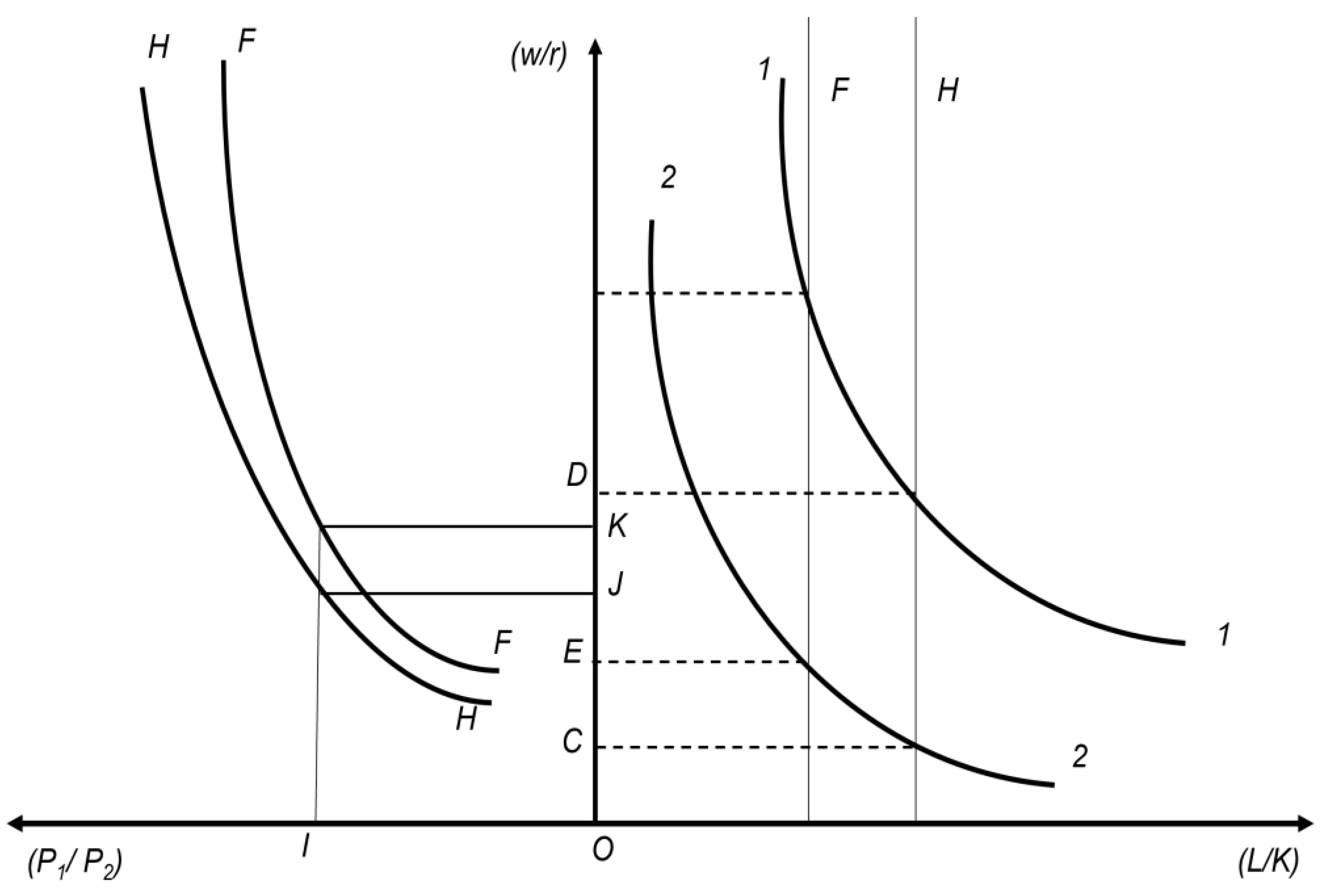
Under the above assumptions, the commodity trade equalises commodity prices. It is of interest to derive, under the above assumptions, the relationships among relative commodity prices, relative factor prices, and factor proportions.

This can be seen in Figure 1. The right-hand side of the figure is the same as that in the H-O-S case since the production functions of the two countries are identical, apart from the multiplicative scalar $\gamma$. When the ratio $\frac{\mathsf{\pi }}{\left(w/r\right)}$ (where $\mathsf{\pi }$ is the factor intensity, w and r are the prices of labour and capital, respectively, and P1 and P2 are the prices of commodities 1 and 2, respectively), $\gamma \mathrm{s}$ cancels out because ${\mathsf{\pi }}_i=\frac{{\gamma }_i{\alpha }_{iL}}{{\gamma }_i{\alpha }_{iK}}=\frac{{\alpha }_{iL}}{{\alpha }_{iK}}$ (from the assumption of homogeneity in production functions). Additionally, $w_i={\gamma }_i\frac{\partial f_i}{\partial L_i}$ and $r_i={\gamma }_i\frac{\partial f_i}{\partial K_i}$. Consequently, when calculating the ratio $\left(\frac{w}{r}\right)$, $\gamma$s cancels out. Therefore, $\frac{\mathsf{\pi }}{\left(w/r\right)}$ is independent of $\gamma$s.

As shown, Figure 1 assumes that commodity 1 is more labour-intensive than commodity 2. The two curves do not cross since it was assumed that there are no factor intensity reversals.

The relationship between the relative prices of commodities and relative factor prices will now be examined, starting with the prices of goods 1 and 2:

$$P_1{\gamma }_1=w{\alpha }_{1L}+r{\alpha }_{1K}$$

(2)

And

$$P_2 {\gamma }_2 = w{\alpha }_{2L} +r{\alpha }_{2K}$$

(3)

where w is the wage rate, r denotes the interest rate, and $\alpha$s are the input coefficients of production (they indicate the production factor units necessary to produce one unit of final output). From Equations (2) and (3), the price ratio of the two commodities can be derived as follows:

$$\frac{P_1}{P_2}=\frac{{\gamma }_2\left(w{\alpha }_{1L}+r{\alpha }_{1K}\right)}{{\gamma }_1\left(w{\alpha }_{2L}+r{\alpha }_{2K}\right)}=\frac{{\gamma }_2}{{\gamma }_1}\frac{\frac{w}{r}{\alpha }_{1L}+{\alpha }_{1K}}{\frac{w}{r}{\alpha }_{2L}+{\alpha }_{2K}}$$

(4)

Differentiating $\left(\frac{P_1}{P_2}\right)$ in (4) with respect to $\left(\frac{w}{r}\right)$, after several calculations, the following is derived:

$$\frac{d\left(\frac{P_1}{P_2}\right)}{d\left(\frac{w}{r}\right)}=\frac{{\gamma }_2}{{\gamma }_1}\frac{{\alpha }_{1K}}{{\alpha }_{2K}}\frac{{\mathsf{\pi }}_1-{\mathsf{\pi }}_2}{{\left(\frac{w}{r}{\mathsf{\pi }}_2+1\right)}^2}$$

(5)

where ${\mathsf{\pi }}_1=\frac{{\alpha }_{1L}}{{\alpha }_{1K}}$ and ${\mathsf{\pi }}_2=\frac{{\alpha }_{2L}}{{\alpha }_{2K}}$.

Relationship (5)3 is always greater than zero since, by assumption, commodity 1 is more labour-intensive than commodity 2 (${\mathsf{\pi }}_1>{\mathsf{\pi }}_2$), and all other terms in (5) are positive. Therefore, the commodity price ratio $\left(\frac{P_1}{P_2}\right)$ is a strictly increasing function of the factor–price ratio $\left(\frac{w}{r}\right)$.

However, the relationship between relative commodity prices and relative factor prices is not independent of $\gamma$s. Since $\gamma$s differs between countries, it is expected that, unlike in the case of the H-O-S theory, the relation between $\left(\frac{P_1}{P_2}\right)$ and $\left(\frac{w}{r}\right)$ in the two countries is represented by different curves. Therefore, the left-hand side of Figure 1 will generally be different from that in the H-O-S theory and will depend on the value of the $\gamma$s.

Three cases can be distinguished in this simple two-country, two-commodity, two-factor model:

• $\frac{{\gamma }_1^H}{{\gamma }_2^H}<\frac{{\gamma }_1^F}{{\gamma }_2^F}$, where the superscripts H and F denote the home country and the foreign country, respectively. This case is shown in Figure 1. From relationship (4), we have the following:

$${\left(\frac{P_1}{P_2}\right)}^H=\frac{{\gamma }_2^H}{{\gamma }_1^H}\frac{\frac{w}{r}{\alpha }_{1L}+{\alpha }_{1K}}{\frac{w}{r}{\alpha }_{2L}+{\alpha }_{2K}}$$

(6)

for country H and

$${\left(\frac{P_1}{P_2}\right)}^F=\frac{{\gamma }_2^F}{{\gamma }_1^F}\frac{\frac{w}{r}{\alpha }_{1L}+{\alpha }_{1K}}{\frac{w}{r}{\alpha }_{2L}+{\alpha }_{2K}}$$

(7)

for country F. Now,

$$\frac{{\gamma }_1^H}{{\gamma }_2^H}<\frac{{\gamma }_1^F}{{\gamma }_2^F}\iff \frac{{\gamma }_2^H}{{\gamma }_1^H}>\frac{{\gamma }_2^F}{{\gamma }_1^F},$$

where, at the same relative factor–price ratio, country H’s commodity price ratio ${\left(\frac{P_1}{P_2}\right)}^H$ will be greater than that of country F’s ${\left(\frac{P_1}{P_2}\right)}^F$ (since the $\alpha$ coefficients are the same for the two countries by assumption), or, because commodity prices equalise after the introduction of trade, at the same commodity price ratio, country F’s relative factor–price ratio is greater than that of country H. From relationship (5), in the case where $\frac{{\gamma }_1^H}{{\gamma }_2^H}<\frac{{\gamma }_1^F}{{\gamma }_2^F}$, the following is derived:

$${\left(\frac{d\left(\frac{P_1}{P_2}\right)}{d\left(\frac{w}{r}\right)}\right)}^H>{\left(\frac{d\left(\frac{P_1}{P_2}\right)}{d\left(\frac{w}{r}\right)}\right)}^F$$

which implies that the curve denoting the relationship between $\left(\frac{P_1}{P_2}\right)$ and $\left(\frac{w}{r}\right)$, as shown in Figure 1, for country F, will be steeper than that for country H. In Figure 1, the curve FF denotes the relationship between the commodity price ratio and factor price ratio in country F and the curve HH in country H. The two curves (HH and FF) do not intersect because relationships (6) and (7) ensure that for the same commodity price ratio, the factor price ratio in country F will always be higher, in a fixed proportion, than that in country H.

• $\frac{{\gamma }_1^H}{{\gamma }_2^H}>\frac{{\gamma }_1^F}{{\gamma }_2^F}$; this is the same as in the first case, with the only difference being that in Figure 1, the curve FF will now represent country H, and the curve HH will represent country F.
• $\frac{{\gamma }_1^H}{{\gamma }_2^H}=\frac{{\gamma }_1^F}{{\gamma }_2^F}$; in this case, HH and FF on the left-hand side of Figure 1 will coincide, and the figure will be the same as that of the H-O-S theory case. In this case, Samuelson’s factor price equalization theorem (Samuelson 1949) holds; Samuelson (1948, 1949).

3.1. The Pattern of Trade with Identical Relative Factor Endowments

We will now examine what can be predicted for the pattern of trade between the countries if production functions are of the form described by (1). Let us consider two countries, H and F, under the assumptions set forth in Section 2. To determine the production possibility frontiers of the two economies, we can examine country H at two different time points, introducing the characteristic differences of country F at the second time point. Therefore, assume that the production functions of the two activities at time t are $Q_1={\gamma }_1{f}_1\left(K_1,L_1\right)$ and $Q_2={\gamma }_2{f}_2\left(K_2,L_2\right)$, ${\gamma }_1={\gamma }_2$, and that commodity 1 is the labour-intensive commodity. At time $t+1$, there is a change in the production function, and ${\gamma }_2$ becomes greater than ${\gamma }_1$. The effects in industry 2 would have been the same as those in industry 2 had they experienced Hicks’ neutral technical progress.

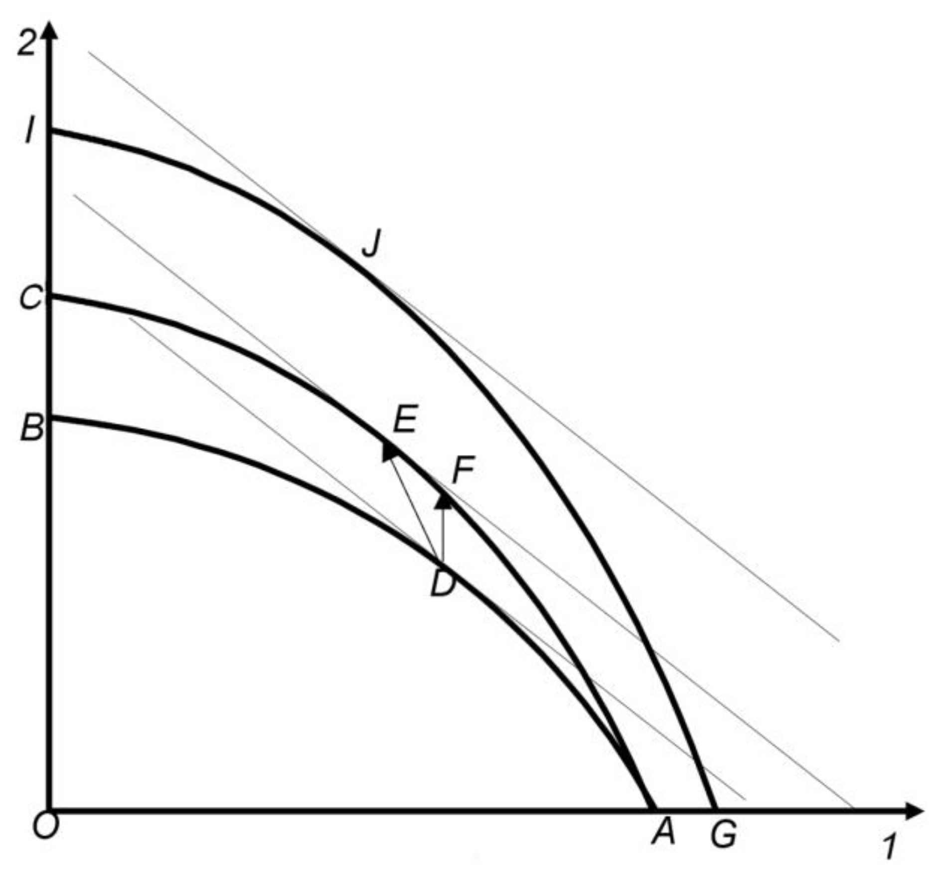
With the experience of such technical progress, industry 2’s isoquants will be renumbered, with each isoquant corresponding to a higher output after the change than before. The production possibility frontier will shift outward, as illustrated in Figure 2. Curve AB is the country’s production possibility frontier at time t, and curve AC is the production possibility frontier after the change at time $t+1$.

If the commodity–price ratio is given by the slope of the country’s pre-trade production possibility frontier at point D, then the price ratio will be assumed to remain the same after the change, with the new production point being point E. At point E, the output of commodity 1 has fallen absolutely, and the output of 2 has increased.

On the other hand, if the factor–price ratio is kept constant at the pre-change level, the production point would shift from D to F. However, at F, the slope of the production possibility frontier is steeper than the slope at D; therefore, at any given factor price, commodity 2 becomes relatively cheaper after the change in industry 2.

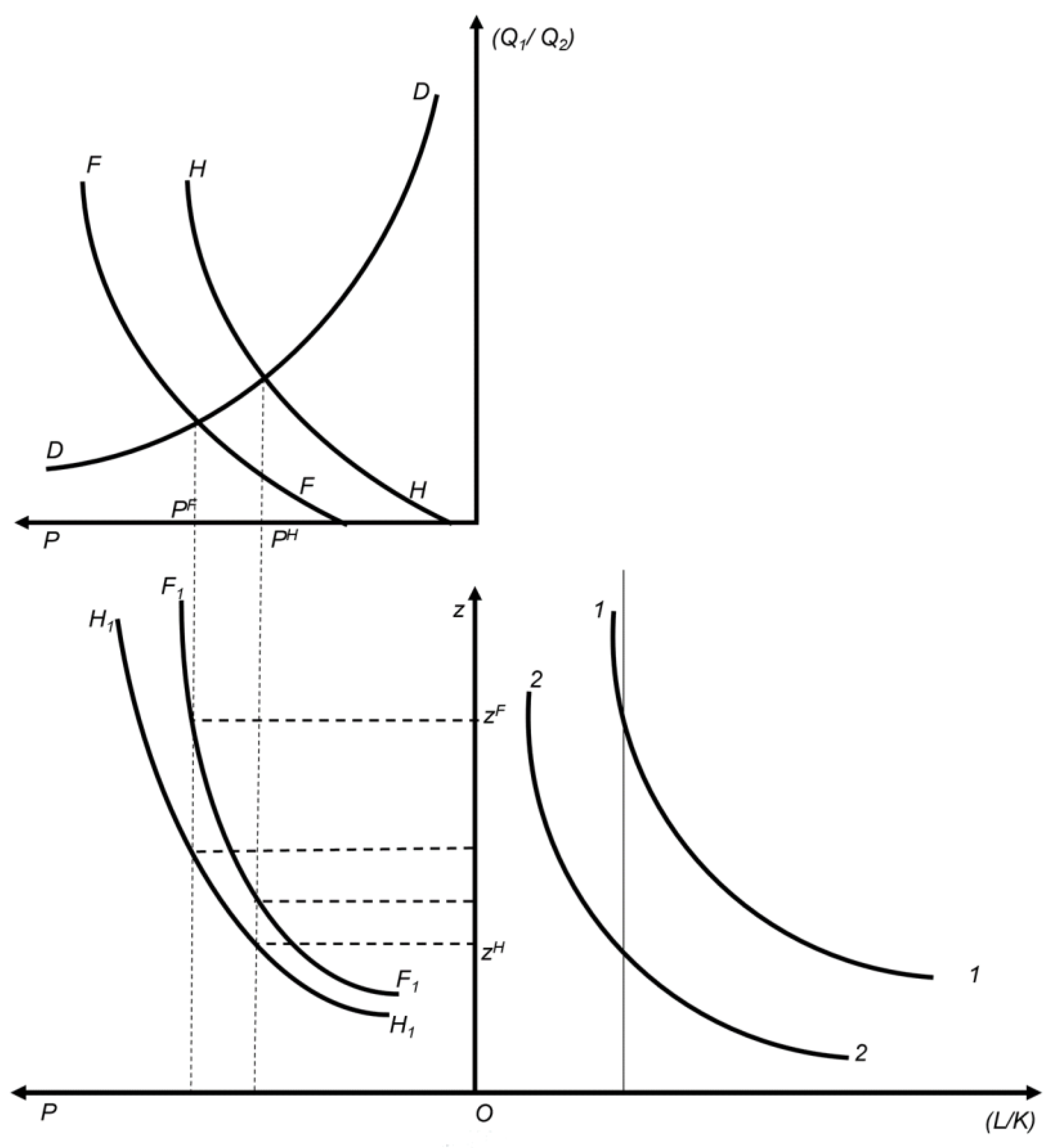
From the above analysis, the relative supply curves of the country before and after the change in industry 2 can be derived (the relative supply curve shows how relative output, with full employment of both factors, varies with relative commodity prices). Before the change, the relative supply curve is depicted by the HH curve (Figure 3). In the above discussion, it has been shown that after the change, the output of commodity 1 will fall, and the output of 2 will increase if the relative commodity prices remain the same (at the same $\left(\frac{P_1}{P_2}\right)$, the ratio will correspond to a lower $\left(\frac{Q_1}{Q_2}\right)$ ratio); alternatively, if prices are allowed to change commodity 2, they will become cheaper relative to commodity 1 (to the same $\left(\frac{Q_1}{Q_2}\right)$, the ratio will correspond to a higher $\left(\frac{P_1}{P_2}\right)$ ratio). This means that the relative supply curve must move to the left of curve HH in Figure 3.

Instead of considering the same economy at two different time points, we consider two different countries, $H$ and $F$, where country $F$ has the characteristics of country $H$ at time $t+1$ (after the change); then, the relative supply curves of the two countries are depicted by the curves HH and FF in Figure 3. At this point, the only difference between the two economies is their described difference in production functions. The two economies are assumed to have identical overall factor-to-endowment ratios, as presented in Figure 3.

If the relative demand curve, DD, which represents the proportion of commodities consumed as a function of relative price, is introduced in this figure, and under the assumption that the relative demand curve is the same for the two countries (the typical assumption for demand in the neoclassical trade model), the pre-trade price ratios in the two countries can be found. In Figure 3, the equilibrium pre-trade price ratio for country $H$ is $P^H$, and that for country F is $P^F$.

Trade can only occur at a price ratio lying in the interval $P^H{P}^F$, because at any other price ratio, the two countries will have an excess supply of the same commodity (at a price ratio greater than $P^F$, there will be an excess supply of commodity 1 at prices lower than $P^H$ and there will be an excess supply of commodity 2). Clearly, at a price ratio lying in the interval $P^H{P}^F$, country H will export commodity 1, and country F will export commodity 2.

3.2. The Pattern of Trade with Different Relative Factor Endowments

The above-described model is a simple way of introducing a second factor of production into the classical model. Thus far, it has been assumed that the relative factor endowments of the two countries are identical. The pattern of trade in this model will be examined now by assuming that the relative factor endowments of the two countries are different, and this can be done by studying the validity of the H-O-S theorem in this model. The two countries are assumed to have identical factor-to-endowment ratios. We will now examine whether the price form of the H-O-S theorem4 is valid. If we assume that $\frac{{\gamma }_1^H}{{\gamma }_2^H}<\frac{{\gamma }_1^F}{{\gamma }_2^F}$, which is the case in Figure 3, then the country with the lower pre-trade commodity price ratio is also the country with the lower pre-trade factor–price ratio $\left(\frac{w}{r}\right)$ since the corresponding factor–price ratio of commodity price ratio $P^H$ is $z^H$ and that of $P^F$ is $z^F$. In this case, $z^H$ will always be smaller than $z^F$, and the price form of the H-O-S theorem will be valid.

Suppose now that the two counties do not have identical factor–endowment ratios and that H is more labour-abundant than country F. In this case, the pattern of trade, as indicated by the $\gamma$s, changes (i.e., their TFP differences), and Figure 3 is altered accordingly. We can examine the new pattern of trade with the help of the Rybczynski theorem (Rybczynski 1955): first, it will be assumed that the two countries have identical factor endowment ratios; then, it will be assumed that one country becomes relatively more abundant in one factor than the other by increasing that factor. Suppose that, in Figure 2, which describes country H before and after the change in $\gamma$s, after the change, the country’s capital endowment is increased; therefore, the country becomes more capital-abundant relative to its previous position.

According to the Rybczynski theorem, this will cause the production possibility frontier to move to the position GI. The production of commodity 2 will increase, and the production of commodity 1 will decrease under the assumption that the same rates of substitution in production before and after the increase in the factor are maintained. Commodity prices are also assumed to remain constant. The new production point will be point J on curve GI in Figure 2.

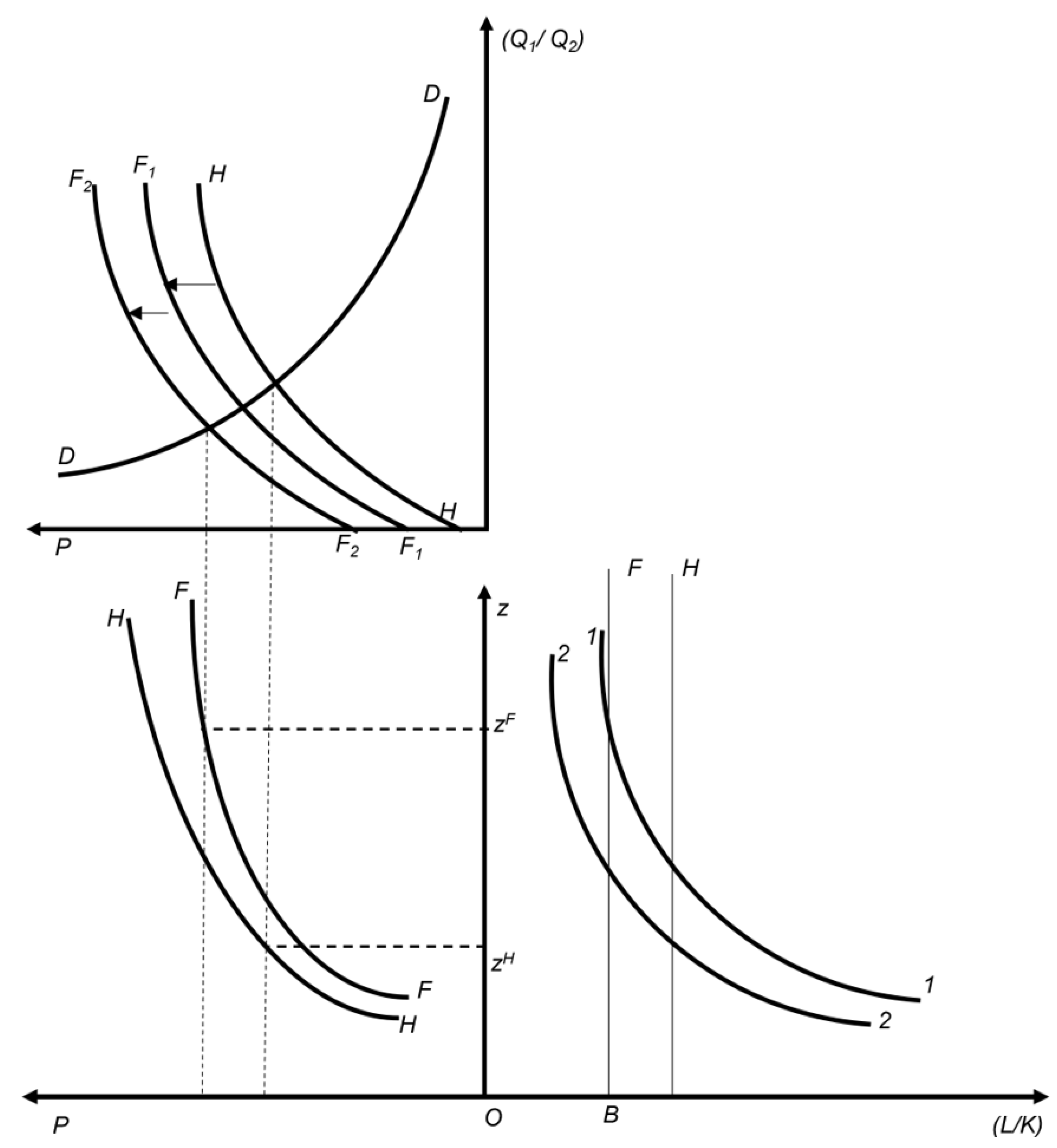
Figure 3 will also be modified after the change in capital endowment (this is shown in Figure 4). On the right-hand side of Figure 4, the new factor endowment ratio is represented by the distance OB. Additionally, the relative supply curve moves further to the left to the position $F_2{F}_2$, reinforcing the effect of the change in $\gamma$s.

In this particular case, both the quantity and the price form of the H-O-S theorem are valid because country H, which is a labour-abundant country, exports commodity 1 (which is a labour-intensive commodity), and country F, which is a capital-abundant country, exports commodity 2 (which is a capital-intensive commodity). Additionally, country H, which has a lower pre-trade commodity price ratio, has a lower pre-trade factor–price ratio. However, in general, the H-O-S is not generally valid in either of its forms because the ‘differential’ $\gamma$ effect and the ‘Rybczynski’ effect on the relative supply curve may reinforce each other, causing the relative supply curve to move in one direction only (in which case the H-O-S theorem will be valid in both its forms); alternatively, they may offset each other, moving the relative supply curve in opposite directions.

Additionally, because of the ‘Rybczynski’ effect, the ranking of commodities according to their $\gamma$ ratio in two countries will not always be in accordance with the ranking of commodities according to their autarky price ratios in two countries, and the Ricardian hypothesis will not be logically valid. Therefore, the ranking of commodities according to their $\gamma$ ratios is not sufficient for predicting the pattern of trade; rather, their ranking according to their factor intensities and the ranking of countries according to their relative factor endowments must be examined. In the two-country, two-commodity, two-factor model, if $\frac{{\alpha }_{1L}}{{\alpha }_{1K}}>\frac{{\alpha }_{2L}}{{\alpha }_{2K}}$ and $\frac{\overline{L^H}}{\overline{K^H}}<\frac{\overline{L^F}}{\overline{K^F}}$, then when $\frac{{\gamma }_1^H}{{\gamma }_2^H}<\frac{{\gamma }_1^F}{{\gamma }_2^F}$ (or $\frac{{\gamma }_1^H}{{\gamma }_1^F}<\frac{{\gamma }_2^H}{{\gamma }_2^F}$), country H will export commodity 1 and import commodity 2, while country F will export 2 and import 1.5 The pattern of trade is indeterminate if one or more inequalities are not satisfied.

Therefore, the pattern of trade between two countries, when the production functions are different among countries for an identical activity (i.e., according to the fundamental assumption of the classical trade model), but the only difference would be a multiplicative scalar of the testable hypothesis, is constructed as follows:

$${\gamma }_i^H/{\gamma }_i^F<{\gamma }_j^H/{\gamma }_j^F;$$

(8)

$$i=1,\dots ,m j=m+1,\dots ,n$$

where commodities $i=1,\dots ,m$ are country H’s exports and commodities $i=m+1,\dots ,n$ are its imports when the countries have identical factor–endowment ratios. The ratio of the $\gamma$s also predicts the pattern of trade between two countries when the two countries have different factor-to-endowment ratios; however, in this case, a further condition is needed: the above ranking is the opposite of their ranking according to their factor intensities (the $\gamma$s should be constructed in such a way that those of the labour-abundant country are placed on the numerator, those of the capital-abundant country are placed on the denominator, and those the capital input coefficients of production are placed on the numerator when constructing the factor intensities).

Concludingly, the theory of the proposed model of trade predicts the pattern of trade between two countries by the gamma ratios when these are correlated with the labour–capital ratios. This derives from and tests the empirical validity of the model; the pattern of trade between two countries is predicted by the ratios of the gamma parameters of each sector for each country (rank test between the export–import ratio and the gamma ratio) when the gamma ratios are correlated with the labour–capital ratios (rank test between the gamma ratios and the labour–capital ratios).

4. Empirical Evidence

In this chapter, the model developed in Section 3 is tested using real-world data. The relationship between the $\gamma$- and α-ratios and between the $\gamma$-ratios and the import-to-exports (X/M) ratio will be examined to test the validity of the model to explain trade flows in the real world, in the bilateral relationship among Germany (the home country) and Russia and the Czech Republic (the foreign countries).

Over the past two decades, Germany has emerged as Russia’s primary trading partner, particularly in sectors like energy and manufacturing. Understanding this relation is crucial for evaluating Europe’s energy security, given Russia’s pivotal role as a major energy supplier to Germany. In particular, 2014 is noteworthy due to Russia’s annexation of Crimea, which shaped global perceptions and impacted international relations. Thus, prompted by this annexation, we aim to investigate the responsiveness of this model under conditions characterised by trade impediments.

The geographical proximity between the Czech Republic and Germany plays a pivotal role in shaping economic ties due to the reduced transportation costs and the absence of trade impediments. The Czech Republic has experienced significant economic transformation since joining the EU in 2004, after the Soviet era; thus, understanding their trade is essential for comprehending the evolving economic landscape in Central Europe.

Therefore, the relationship of these countries with Germany constitutes an example to comprehend the international trade nexus in Eastern parts of Europe. The two case studies are used to demonstrate the ability of our trade model to explain trade flows in the real world. However, we expect the model to provide better results with the Germany–Czech Republic trade relations rather than the Germany–Russia case since trade impediments were, in effect, on the latter, which do not allow trade to equalise commodity prices.

To test this model, the variables associated with the trade patterns, as indicated in Section 3 above, must first be specified. The first step is to calculate the factor intensities (α_i) for each country. For the purposes of the analysis, the ISIC classification of 24 production sectors was used. The 24 production sectors were classified into four broad categories: agricultural, energy, manufacturing, and services.

Table 1. Description of variables and sources.

Variables	Description	Sources
Output (Y)	Gross output at basic prices	WIOD SEA files
Labour1 (L1)	Number of employees engaged	WIOD SEA files
Labour2 (L2)	Compensation of employees	WIOD SEA files
Capital (K)	Net capital stock	Authors’ calculations and WIOD SEA files

Source: Authors’ construction and WIOD database. L¹ represent the “Number of employees engaged and L² represent the “Compensation of employees”. Both measures of Labour are used for robustness.

provides a detailed list of the data used and sources regarding labour, capital, and output series for each sector available from the (Timmer et al. 2015) database for 20146.

To calculate factor intensities, the labour and capital per unit of output were calculated, i.e., ${\alpha }_{i,K}=\frac{K}{Y}$ and ${\alpha }_{i,L}=\frac{L^i}{Y}$; i = 1, 27 for each country and each sector. Next, we need to determine the countries’ relative abundance in factor endowments, i.e., which country is labour-abundant, and which is capital-abundant, to derive the $\frac{\overline{L^H}}{\overline{K^H}}\mathrm{and} \frac{\overline{L^F}}{\overline{K^F}}$ ratios. To conduct this, the sectoral total of “Total hours worked by employees” aggregated for all sectors was divided by the sectoral total of “Net capital stock” aggregated for all sectors. This resulted in a higher labour-to-capital ratio for Russia and the Czech Republic than for Germany, indicating that these countries are labour-abundant, while Germany is a capital-abundant country.

A CES-type production function can be used to describe (1), with labour and capital as its primary inputs, of the following form:

$$Q_i^j={\gamma }_i^j{\left(a_{i K}^j{K}_i^{j \sigma }+a_{i L}^j{L}_i^{j \sigma }\right)}^{\raisebox{1ex}{$1$}\!\left/ \!\raisebox{-1ex}{$\sigma $}\right.}; i=1,\dots ,24, j=H, F$$

(9)

where Q denotes output, i denotes activity i, j denotes country, j, L, K denotes the two primary factors of production, and γ is a scalar.

In (9), $\gamma$ is the multiplicative scalar, measuring the sectoral TFP, which allows production functions to be different between two countries for the same sector; $a_K$ and $a_L$ are the input coefficients of capital and labour, respectively; and σ is the substitution elasticity parameter in the production function that has been estimated for each sector separately. Note that the $\alpha$s of the same sector are different between countries because relative factor prices and, consequently, factor intensities, are different (see Section 3 and Figure 1). Furthermore, from the basic assumption of the model (Equation (1)), production technologies are the same across countries differing only to the multiplicative scalar, γ; therefore, the σs and the elasticities of substitution for the same sector across countries are the same.

Before proceeding with the calculation of the $\gamma$s, the estimation of the elasticity parameters and the calculation of the elasticities of substitution must be performed. Equation (9) is estimated for each sector separately using the nonlinear least squares approach (see Bertsatos and Tsounis 2023). For the nonlinear estimation, an initial value of 0.5 was assumed for the iterative algorithm.

Table 2. Substitution elasticity parameters and elasticity of factor substitution by sector.

Sector	σ	Elasticity of Substitution
Agricultural
Agriculture, forestry, and fishing	0.070 *	0.935
Mining and quarrying of non-energy-producing products	0.306 *	0.766
Energy
Mining and extraction of energy-producing products	0.210 *	0.826
Coke and refined petroleum products	0.124 *	0.890
Electricity, gas, water supply, sewerage, waste, and remediation services	0.115 *	0.897
Manufacturing
Food products, beverages, and tobacco	0.159 *	0.863
Textiles, wearing apparel, leather, and related products	0.142 *	0.876
Wood and products of wood and cork	0.029 *	0.972
Paper products, printing chemicals, and pharmaceutical products	0.038 *	0.963
Chemicals and pharmaceutical products	0.145 *	0.873
Rubber and plastic products	0.097 *	0.912
Other non-metallic mineral products	0.119 *	0.894
Basic metals	0.058 *	0.945
Computer, electronic, and optical products	0.164 *	0.859
Machinery and equipment, NEC.	0.134 *	0.882
Motor vehicles, trailers, and semitrailers	0.160 *	0.862
Other manufacturing; repair and installation of machinery and equipment	0.219 *	0.820
Construction	0.266 *	0.790
Services
Wholesale and retail trade; repair of motor vehicles	0.042 *	0.960
Transportation and storage	0.021 *	0.979
Telecommunications	0.022 *	0.978
Financial and insurance activities	0.099 *	0.910
Public admin. and defence; compulsory social security	0.101 *	0.908
Arts, entertainment, recreation, and other service activities	0.199 *	0.834

Source: Authors’ estimates/note: * denotes statistical significance at least at the 5% level.

reports the estimated substitution parameters along with the elasticities of substitution of the CES production function. The elasticities of substitution determine how easy or how difficult it is for a sector to adjust its production in response to factor prices. By estimating the elasticity parameter σ, the elasticities of substitution are easy to calculate by $\frac{1}{1+\sigma }$. For the convenience of the reader,

Table A1. Symbols and definitions.

Symbol	Definition
$Q_i^j$	Output of activity i for country j
${\gamma }_i^j$	Multiplicative scalar (sector’s i TFP for country j)
$L_i^j$	Labour input for activity i and country j
$K_i^j$	Capital input for activity i and country j
${\pi }_i$	Factor intensity for commodity i
w	Price of labour
r	Price of capital
P1	Price of commodity 1
P2	Price of commodity 2
${\alpha }_{iL}$	Input coefficient of labour for commodity i
${\alpha }_{iK}$	Input coefficient of capital for commodity i
H	Indicator for the home country (Germany in the Section 4)
F	Indicator for a foreign country (Russia or the Czech Republic in the Section 4)
$P^H$	Equilibrium pre-trade price ratio for country H
$P^F$	Equilibrium pre-trade price ratio for country F
$z^H$	Factor–price ratio for country H
$z^F$	Factor–price ratio for country F
$\overline{L^H}$	Labour endowment of the home country
$\overline{K^H}$	Capital endowment of the home country
$\overline{L^F}$	Labour endowment of the foreign country
$\overline{K^F}$	Capital endowment of the foreign country
σ	Substitution elasticity parameter

Source: Authors’ construction.

in the Appendix A specifically explains the variables used in the empirical implementation.

When the substitution parameters are less than one-half, the substitution elasticity values are high. Small value elasticities of substitution indicate that a large amount of labour is required to substitute one unit of capital while maintaining constant production. On the contrary, when substitution elasticities are close to one, it is easier to substitute labour with capital and vice versa.

By fitting the elasticities of substitution for each sector in Equation (9), the $\gamma$s were calculated as scale parameters. Next, the $\gamma$-ratios are calculated as the ratio of a sector’s gamma of the labour-abundant country (Czech Republic or Russia) to the corresponding sector’s gamma of the capital-abundant country (Germany). Finally, the export-to-import ratio of Russia and the Czech Republic to Germany must be calculated.

The data for imports and exports were obtained from the Eurostat (Eurostat 2023) database. To construct this ratio, Russia’s and the Czech Republic’s exports to Germany are placed in the numerator, while Germany’s imports from Russia and the Czech Republic are placed in the denominator.

Since all the variables needed are specified, a rank test can be performed to establish the rank correlation between the ranking of industries according to their exports or imports and their ranking according to their TFP ratio (the $\gamma$ ratio), as in (8), who first ensured that the ranking of sectors according to the $\gamma$ ratio is similar to the ranking according to the factor intensities ($\gamma$s are constructed in such a way that those of the labour-abundant country are placed on the numerator, those of the capital-abundant country are placed on the denominator, and the capital input coefficients of production are placed on the numerator when constructing the factor intensities).8 For the rank test, the Spearman rank correlation coefficient is used to first assess the feasibility of the use of the rank test for the direction of trade (rank test between $\gamma$- and the α-ratio); then, if this test provides valid results, the strength and direction of the trade pattern between the $\gamma$-ratio and the import-to-export ratio for bilateral trade relationships between each country with Germany as their trading partner are assessed.

The coefficients of the Spearman rank correlation in each set between the two variables and the ranking of sectors are reported in

Table 3. Spearman rank correlation test between $\gamma$-ratios and the α-ratios for each country.

Russia-Germany					Czech Republic-Germany
Sectors	Ratio		Ratio		Ratio		Rank
	γ	α	γ	α	γ	α	γ	α
Agriculture
Agriculture, forestry, and fishing	3.960	19.036	19	21	30.545	0.099	4	22
Mining and quarrying of non-energy-producing products	6.848	13.092	21	20	567.59	0.614	22	23
Energy
Mining and extraction of energy-producing products	19,630.6	38.763	24	23	240.92	1.818	14	24
Coke and refined petroleum products	0.751	2.714	12	8	21,992.4	0.033	24	7
Electricity, gas, water supply, sewerage, waste, and remediation services	303.38	43.458	23	24	37.031	0.032	5	6
Manufacturing
Food products, beverages, and tobacco	1.306	1.919	13	2	273.97	0.031	17	5
Textiles, wearing apparel, leather, and related products	0.294	6.646	7	15	74.20	0.041	9	13
Wood and products of wood and cork	0.152	2.873	3	10	231.04	0.034	13	8
Paper products and printing	0.302	2.163	8	4	122.171	0.020	10	2
Chemicals and pharmaceutical products	2.329	5.535	15	13	271.03	0.079	16	20
Rubber and plastic products	1.757	2.742	14	9	336.23	0.050	19	17
Other non-metallic mineral products	0.409	2.413	9	6	56.91	0.027	8	4
Basic metals	0.480	3.299	10	11	411.18	0.038	21	11
Computer, electronics, and optical equipment	4.356	11.0	20	18	260.86	0.051	15	19
Machinery and equipment, NEC.	0.142	5.234	2	12	198.22	0.051	12	18
Motor vehicles, trailers, and semi-trailers	0.292	5.66	6	14	1214.21	0.083	23	21
Other manufacturing; repair and installation of machinery and equipment	3.571	1.631	18	1	167.33	0.042	11	14
Construction	0.286	2.129	5	3	373.25	0.020	20	3
Services
Wholesale and retail trade; repair of motor vehicles	3.201	8.163	17	17	44.80	0.034	7	9
Transportation and storage	0.009	2.496	1	7	11.61	0.040	3	12
Telecommunications	0.649	12.72	11	19	37.64	0.046	6	15
Financial and insurance activities	3.020	7.857	16	16	286.27	0.046	18	16
Public admin. and defence; compulsory social security	219.3	30.80	22	22	0.606	0.034	1	10
Arts, entertainment, recreation, and other service activities	0.251	2.258	4	5	4.776	0.015	2	1
Spearman Rank Correlation Test
Spearman rank coefficient (rs)	0.62				0.401
Number of observations (n)	24				24
T-statistic	3.706				2.051
Degrees of freedom (DF)	22				22
p-value	0.001 ***				0.049 **

Source: Authors’ calculations; *** and **, indicates p < 0.001 and p < 0.05 respectively.

and

Table 4. Spearman rank correlation test between $\gamma$-ratios and X/M ratios for each country.

Russia-Germany					Czech Republic-Germany
Sectors	Ratio		Ratio		Ratio		Rank
	γ	X/M	γ	X/M	γ	X/M	γ	X/M
Agriculture
Agriculture, forestry, and fishing	3.961	0.462	19	12	30.54	3.80	4	22
Mining and quarrying of non-energy-producing products	6.848	4.523	21	18	567.59	0.753	22	9
Energy
Mining and extraction of energy-producing products	19,630.6	56,726.1	24	24	240.92	154.75	14	24
Coke and refined petroleum products	0.751	12.662	12	21	21,992.4	0.544	24	4
Electricity, gas, water supply, sewerage, waste, and remediation services	303.3	2934.4	23	23	37.031	1.273	5	14
Manufacturing
Food products, beverages, and tobacco	1.306	0.112	13	5	273.97	0.033	17	2
Textiles, wearing apparel, leather, and related products	0.295	0.102	7	4	74.20	0.990	9	11
Wood and products of wood and cork	0.152	2.549	3	17	231.04	2.843	13	21
Paper products and printing	0.302	0.260	8	11	122.17	0.598	10	5
Chemicals and pharmaceutical products	2.329	0.126	15	7	271.03	0.624	16	6
Rubber and plastic products	1.757	0.147	14	8	336.23	1.045	19	12
Other non-metallic mineral products	0.409	0.161	9	9	56.91	1.484	8	15
Basic metals	0.480	4.586	10	19	411.18	0.633	21	7
Computer, electronics, and optical equipment	4.356	13.106	20	22	260.86	1.878	15	16
Machinery and equipment, NEC.	0.143	0.073	2	3	198.22	0.941	12	10
Motor vehicles, trailers, and semi-trailers	0.293	0.049	6	2	1214.21	1.965	23	17
Other manufacturing; repair and installation of machinery and equipment	3.571	0.028	18	1	167.33	2.649	11	20
Construction	0.286	0.189	5	10	373.25	0.011	20	1
Services
Wholesale and retail trade; repair of motor vehicles	3.201	1.313	17	15	44.80	2.089	7	18
Transportation and storage	0.010	1.821	1	16	11.61	2.412	3	19
Telecommunications	0.650	1.186	11	14	37.64	1.120	6	13
Financial and insurance activities	3.021	0.116	16	6	286.27	0.488	18	3
Public admin. and defence; compulsory social security	219.3	0.542	22	13	0.606	4.600	1	23
Arts, entertainment, recreation, and other service activities	0.251	5.001	4	20	4.776	0.731	2	8
Spearman Rank Correlation Test
Spearman rank coefficient (rs)	0.301				0.495
Number of observations (n)	24				24
T-statistic	1.479				2.676
Degrees of freedom (DF)	22				22
p-value	0.047 **				0.013 **

Source: Authors’ calculations; ** indicates p < 0.05.

for each country, respectively. The correlation is positive and statistically significant for both cases.

As mentioned in Section 3 above, the ranking of commodities according to their $\gamma$-ratio is not sufficient for predicting the pattern of trade. Thus, the rankings according to factor intensity and rankings according to relative factor endowment must be examined.

According to the null hypothesis (H0) in the Spearman rank correlation test, there is no monotonic relationship between the two sets of variables examined, while the alternative hypothesis (H1) suggests that there is a significant monotonic relationship. For the case of the Czech Republic and Germany, Table 3 shows that the value of the Spearman rank correlation coefficient is equal to 0.401, indicating a moderate to high positive correlation between $\gamma$- and the α-ratio. Finally, for the case of Russia, the results show that the Spearman correlation coefficient is equal to 0.62, indicating a high correlation between $\gamma$- and the α-ratio. The results of the factor intensities to the $\gamma$-ratio rank test, i.e., the necessary condition, validate that we proceed with the trade pattern rank test for each country case.

In Table 4, the correlation coefficients between $\gamma$- and the export-to-import ratio are presented. The correlation coefficient for the case of the Czech Republic and Germany was equal to 0.495 and statistically significant at the 5% level. On the other hand, the correlation coefficient for Russia is equal to 0.301 and it is statistically significant at the 5% level. We conclude that TFP differences can be used as a basis for explaining comparative advantages and, therefore, the pattern of trade exhibited between two countries.

In the context of the Czech Republic and Germany, the Spearman correlation coefficient explains a larger share of trade dynamics compared to the case with Russia, indicative of reduced transportation costs attributed to the geographical proximity of the two countries and the absence of trade impediments that allow commodity–price equalisation. Conversely, the correlation coefficient observed between Russia and Germany registers as lower, primarily attributable to the EU sanctions imposed on Russia for the annexation of Crimea in 2014.

5. Conclusions and Policy Implications

In this paper, we have shown that in the case where production functions are described by relationship (1), and under the assumption that the two countries have identical factor–endowment ratios, differences in TFP at the industry level between countries can be used to predict the pattern of trade. Furthermore, we found that if countries have different factor-to-endowment ratios, a further condition is required, i.e., the industry TFP ratios (i.e., $\gamma$ ratios) must predict the pattern of trade according to their ranking by factor intensities.

More specifically, the Spearman rank correlation coefficient was used to test the relationship between the $\gamma$- and α-ratios, as well as the $\gamma$-ratios and the import-to-export ratio. Additionally, two Spearman rank correlation coefficients were calculated. The first test was used to assess the feasibility of using the rank test for the direction of trade (rank test between $\gamma$- and the α-ratio); as soon as this test yielded valid results, the strength of the trade pattern between the $\gamma$-ratio and the import-to-export ratio could be measured for the bilateral trade relationship between Russia and the Czech Republic, with Germany as their trading partner. The results of the first rank test between $\gamma$- and α-ratios indicated a statistically significant and positive relationship of 0.62 for Russia–Germany and 0.401 for the Czech Republic–Germany. This result validated our decision to proceed with the trade pattern rank test. The correlation coefficient between the $\gamma$- and export-to-import ratios was found to be of the correct sign, equal to 0.301 for Russia–Germany and, 0.495 for the Czech Republic–Germany, implying that the model can predict the direction of trade patterns between the two countries.

The TFP can be used as an analytical tool for assessing and describing the comparative advantage between countries. By quantifying the efficiency with which inputs are transformed into outputs in a country, TFP allows for the identification of relative productivity levels. A higher TFP indicates a comparative advantage in transforming primary manufacturing inputs into goods and services. This measurement aids in identifying the sectors or industries in which the country has a comparative edge. Based on the study’s results, countries can use sectoral TFP estimates to analyse comparative advantages for bilateral trade relations and direct resources to these industries, thereby increasing trade gains. TFP differences, on the other hand, can be used by policymakers to learn more about how countries can enhance their economic growth by better understanding global economic dynamics and trade patterns. Therefore, a thorough analysis of TFP differences between countries can highlight areas of specialisation, which in turn guide trade strategies and inform policy decisions.

The limitations of the trade model presented in this paper, as with every model of economic theory, stem from the assumptions adopted. In our case, it is assumed that trade equalises commodity prices; therefore, there are no trade impediments or transportation costs. Additionally, while the presented model implicitly accounts for the existence of external economies of scale (their effects are incorporated into the γ parameter of the production functions), it does not account for the existence of internal economies of scale that are present when there is monopoly power in a sector.

Further work can be pursued by two paths: first, by attempting to incorporate trade impediments and transportation costs (they both affect the commodity–price equalisation assumption) and second, by conducting an empirical analysis by fitting the new production functions to real-world data from additional countries and testing whether the pattern of trade is compatible with the one predicted by the model.