The Euro Area 12: A Comparative Assessment of Its Member States in the Period 1998–2022

Abstract

The primary objectives of this research are to compare the economic performance of the Member States (MS) in the Euro Area 12 (EA-12) of the European Union (EU) that served as net contributors and net recipients of its budget during the period 1998–2022. The comparison focuses on aspects related to economic growth and the business cycle, exploring the presence of hysteresis. To achieve these objectives, a novel approach is employed, which integrates the analysis of both growth and cycles. This approach involves using the Seemingly Unrelated Regression Equations (SURE) model to estimate a translog production frontier and assess the impact of lagging output gaps on the potential output or capacity for each of the MS considered. The data used to estimate each frontier and analyze growth decomposition consist of quarterly data filtered using the Kalman filter. The results reveal that lagging output gaps, occurring one or two quarters prior, significantly affect the potential output or capacity of the EA-12 MS, thereby supporting the existence of hysteresis. However, the impacts appear to be minimal. Furthermore, the research concludes that changes in total factor productivity (TFP), mainly due to technical change, play a more crucial role in the growth of MS that are net contributors to the EU budget. Conversely, total factor accumulation (TFA), mainly physical capital accumulation, has a more pronounced impact on the growth of MS net recipients from the EU budget. Interestingly, the heterogeneity observed among the EA-12 MS extends beyond the simple division between net contributors and net recipients of the EU budget. This heterogeneity raises questions about the European Central Bank’s (ECB) ability to stabilize the economies of these various MS solely through conventional monetary policy.

1. Introduction

The objectives of this article are two-fold: (i) to analyze the growth of potential output per worker, as well as the changes in the output gap per worker in the EA-12 MS net contributors and net recipients of the European Union (EU) budget, and (ii) to explore the existence of hysteresis or long-lasting effects of shocks within the specified member states (MS). To this end, we employ an innovative empirical approach that integrates the analysis of both growth and cycles.

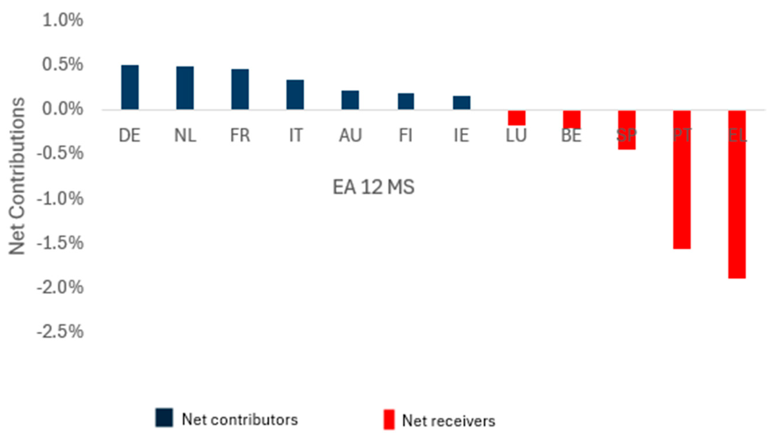
Figure 1 illustrates which of the EA-12 Member States were, on average, net contributors and net recipients of the EU budget, with net contributions expressed as a percentage of their Gross Domestic Product (GDP) during the analyzed period. In order of contribution, Germany, the Netherlands, France, Italy, Austria, Finland, and Ireland were net contributors, while Luxembourg, Belgium, Spain, Portugal, and Greece were net recipients. This order will be considered in the analysis carried out. Its significance lies in the fact that, since the 2008 Global Financial Crisis (GFC), MS that have contributed the most to the EU budget—notably Germany and the Netherlands—have begun to question their net contributions and have elevated this issue to the forefront of the European debate.

We used the SURE model to estimate a translog production frontier (Christensen et al. 1973) and an equation that captures the impacts of lagging output gaps on potential output, for each of the economies under analysis, in the period from 1998 to 2022, in first differences, with quarterly data filtered through the Kalman filter. The Seemingly Unrelated Regression Equations (SURE) model was utilized in the estimation, because the 12 MS belong to the EA-12 and, thus, we expect the error terms to be correlated across equations.

The empirical approach adopted enables us not only to decompose actual and potential output growth per worker into their latent components, but also to accommodate Cerra and Saxena’s new stylized fact of the business cycle (Cerra and Saxena 2008, 2017; Cerra et al. 2023). The new stylized fact posits that, on average, all types of recessions lead to permanent output losses. This results in a downward shift in the GDP trend and permanently reduces the country’s potential output or productive capacity. Such findings imply the existence of hysteresis or lasting impacts of temporary shocks on the trajectory of the economy. Dosi et al. (2018) and Cerra et al. (2023) have undertaken extensive research on hysteresis, its dynamics, and its implications for economic growth and business cycles.

Dosi et al.’s (2018) research illuminates the intricate interplay among firms, workers, and macroeconomic variables. They emphasized the critical importance of understanding hysteresis for designing effective economic policies. In their interpretation, hysteresis arises from the heterogeneous and nonlinear responses of a system characterized by multiple equilibria or path-dependent trajectories. The authors identified coordination failures and persistent effects of aggregate demand on productivity as the primary sources of long-term jumps across multiple growth trajectories. By revealing the intricate dynamics among various macroeconomic variables, they challenged the conventional view that rigid labor markets exacerbate hysteresis. Instead, they highlighted that sustaining aggregate demand during severe downturns can mitigate hysteretic dynamics.

In their literature review, Cerra et al. (2023) identified the development of an alternative business cycle model over the past 25 years. In this model, GDP is history-dependent, and all shocks can have permanent or scarring effects on output—a phenomenon referred to as hysteresis. In the presence of endogenous growth, hysteresis naturally emerges in many business cycle models. To mitigate the scarring effects of shocks, the authors asserted that aggressive and swift action during recessions becomes the optimal policy. However, during expansions, the cost of acting too early due to fears of inflationary pressure can be detrimental, potentially hindering positive developments in the labor market or reducing the economy’s growth potential.

Since 2008, the EU and Euro Area (EA) have been experiencing significant shocks, including the 2008 GFC, the 2020 COVID-19 pandemic, the 2022 Russia–Ukraine war escalation, and the 2023 Israel–Hamas war. Barro and Ursúa (2008) ranked macroeconomic disasters since 1870. If the crisis induced by the 2020 COVID-19 pandemic and the policy response to it were anything like what happened with the 1918 Spanish Flu pandemic, referred to by the authors, the world economy would have experienced one of the worst recessions to date. However, this time was different in the EU and the EA, particularly in terms of the policy reaction to the 2020 COVID-19 pandemic. The EU and EA were still recovering from the 2008 GFC when the 2022 Russian invasion of Ukraine occurred. This hit Germany particularly hard, considering the country’s energy dependence on Russia, and brought by itself inflation to the EU and the EA. That is, this war and the financial speculation related to it have, at least in part, contributed to the latest inflation crisis in the EU and EA. The Israel–Hamas conflict in the Middle East also holds the potential to trigger inflation in the EU and the EA.

This article unfolds as follows. Following this introductory section, Section 2 addresses the ongoing neoclassical debate on hysteresis. It is followed by Section 3, which discusses the effects and expected effects found in the literature of the main shocks suffered by the EA in the period under analysis. Section 4 presents the empirical model and data, while Section 5 yields and discusses the results. Finally, Section 6 concludes the article.

2. The Ongoing Neoclassical Debate Regarding Hysteresis

The disagreement among neoclassical macroeconomists is not new. The New Neoclassical Synthesis (NNS, Goodfriend and King 1997) assumes that demand-side shocks, namely monetary policy, lead to temporary short-term fluctuations in actual GDP around its long-term trend, the effects of which on growth dissipate after some time. The long-term trend is seen as the economy’s production capacity over time, corresponding to the potential or frontier output, which can only be changed by supply-side factors (Lucas 2003). Consequently, the autonomous nature of variations in the trend should not be mistaken for movements along the short-term supply curve itself, as the latter are simply outcomes of present or past changes in aggregate demand (Gordon 1984). However, Campbell and Mankiw (1987), along with Blanchard and Quah (1989), questioned this perspective.

Campbell and Mankiw (1987) investigated the dynamics of economic fluctuations, with a specific focus on differentiating between the permanent and transitory components of real Gross National Product (GNP) fluctuations. Based on post-war quarterly data, the authors found it challenging to refute the notion that real GNP behaves like a persistent random walk with drift. This suggests that shocks to output have a significant and lasting impact, rather than being purely transitory.

Blanchard and Quah (1989) explored the intricate relationship between economic fluctuations, focusing on aggregate demand and supply shocks. They distinguished between supply disturbances (with a permanent effect on output) and demand disturbances (with a transitory effect). The authors acknowledged that quantifying the individual contributions of these disturbances remains challenging. Moreover, their research underscores the critical importance of comprehending the intricate interplay between demand and supply for effective economic policymaking and skillfully managing fluctuations.

The New Keynesian variant of Dynamic Stochastic General Equilibrium (DSGE) models of the business cycle, which has served as the cornerstone for many central banks’ analyses, assumes that temporary shocks, whether affecting demand or supply, do not impact the productive capacity of the economy. Notable examples of these models include works by Clarida et al. (1998), Blanchard and Galí (2007), and Avouyi-Dovi and Sahuc (2016). The 2008 GFC and the 2020 COVID-19 pandemic have raised questions about their empirical validity and highlighted the presence of hysteresis.

The concept of hysteresis has played a central role in contemporary economic discourse. At its core, hysteresis challenges traditional economic logic, as emphasized by Blanchard and Summers (1986), who examined the persistent effects of economic shocks on the trajectory of unemployment. They highlighted that such equilibria may be unstable and fragile, pointing to the complexities inherent in unemployment dynamics.

Expanding upon these perspectives, empirical research by Ball and Onken (2022) provides evidence of hysteresis dynamics across a diverse set of Organization for Economic Cooperation and Development (OECD) countries. Their findings revealed that deviations from the natural rate of unemployment have lasting effects, with decreases in unemployment exhibiting larger long-term impacts. This empirical validation echoes Ball’s (2009) argument that hysteresis fundamentally shapes the long-term behavior of unemployment, particularly in response to shifts in aggregate demand. Moreover, the comprehensive analysis by Cerra et al. (2023) underscores the broader interplay between economic growth, business cycles, and hysteresis effects. Advocating for a unified analytical framework, their research emphasized the need to integrate the persistent impact of shocks on GDP levels into economic models. By highlighting the critical role of active monetary and fiscal policies in mitigating the enduring scars of economic downturns, while leveraging expansions to yield lasting positive effects, Cerra et al.’s (2023) findings provide valuable insights for policymakers grappling with economic stabilization efforts.

Beyond the realm of unemployment, Blanchard et al. (2015) delved into how prolonged recessions can fundamentally alter the trajectory of an economy. This analysis emphasized the imperative of integrating hysteresis effects into macroeconomic frameworks to better understand and address economic fluctuations.

Similarly, Vines and Wills (2018) contributed to the discussion by examining structural factors contributing to hysteresis. Through their research, they proposed targeted policy interventions aimed at mitigating hysteresis’s adverse effects on long-term economic performance. Their recommendations underscore the need for a comprehensive reevaluation of core economic models, incorporating heterogeneity to foster economic stability and growth.

Moreover, Ball (2014) delved into the implications of hysteresis within the context of monetary and fiscal policies, illustrating how such policies can influence long-term economic dynamics. The persistence of economic downturns, caused by hysteresis effects, can lead to enduring challenges, such as elevated unemployment rates or reduced productive capacity. Various monetary and fiscal policy tools, such as interest rate adjustments or government spending initiatives, can impact these long-term economic dynamics. For instance, monetary policies or targeted fiscal stimulus measures help mitigate the effects of hysteresis by stimulating demand and promoting economic recovery. Overall, Ball’s (2014) research sheds light on the role of monetary and fiscal policies in addressing the long-term consequences of hysteresis-induced economic downturns.

Ioannides and Pissarides (2015) delved into the intricacies of the Greek crisis, labor market dynamics, and the impact of hysteresis on employment levels. They contended that Greece’s economic challenges arise from both supply-side and demand-side factors, issues that have persisted since Greece’s accession to the EU in 1981. Throughout the Greek crisis, the sharp decline in demand has been particularly pronounced, exacerbated by austerity measures and wage reductions. These not only compound the demand-side difficulties faced by the Greek economy but also aggravate its underlying structural supply challenges. Additionally, the timing of labor market reforms has played a role in contributing to the crisis. The authors underscore the importance of adopting a balanced approach to tackle both supply and demand issues within the Greek economy.

Yellen (2017) provided valuable insights into hysteresis within monetary policy and uncertainty. The forces driving inflation in the US economy remained uncertain, and the low inflation was likely reflecting factors whose influence should fade over time. However, there were several uncertainties associated with her assessment. Downward pressures on inflation could unexpectedly persist, and the strength of the labor market, inflation expectations, and fundamental forces driving inflation may have been misjudged. Moreover, the persistent low inflation in the US at the time, despite the improvement in labor market conditions, limited the scope for easing monetary policy during normal times.

Costa et al. (2021) employed a vector autoregression (VAR) model to analyze the relationship between the output gap and potential output in Germany and Portugal. Their study illuminated the lasting effects of shocks on potential output within distinct economic contexts. Notably, they explored how country-specific factors, such as business cycle volatility, can influence hysteresis dynamics. Specifically, they discovered that the amplitude of the business cycle and the persistence of shocks are greater in the Portuguese economy than in the German one. The insights gleaned from their analysis provide crucial information for policymakers, enabling them to devise targeted interventions that mitigate adverse effects and promote economic recovery.

Tervala (2021) extended the New Keynesian model to incorporate hysteresis. Hysteresis implies that recessions reduce the level of potential output. Contrary to Lucas (2003), who argued that the welfare costs of business cycles are negligible without hysteresis, Tervala demonstrated that the welfare costs of recessions are significant when hysteresis is considered.

Tervala and Watson (2022) analyzed the output and welfare multipliers of fiscal stimulus during a recession. Transfer payments, public consumption, and investment all have high output and welfare multipliers due to their positive effects on total factor productivity (TFP) in a recessionary environment. Public investment, in particular, has the highest output and welfare multipliers because it positively impacts labor productivity through an increase in the public capital stock. Policymakers should consider these factors when designing effective fiscal stimulus measures during economic downturns. Understanding hysteresis’s impact on welfare costs and the effectiveness of fiscal policies during recessions is crucial for informed policy decisions and societal wellbeing.

The new stylized fact from Cerra and Saxena (2008, 2017) and Cerra et al. (2023) asserts that, on average, all types of recessions lead to permanent output losses. This implies that short-term, temporary shocks have lasting effects on the economy in the long term, rather than being neutral. Such findings provide strong support for the existence of hysteresis.

Cerra and Saxena (2008) examined the role of fiscal and monetary policies in either reversing or perpetuating economic shocks, shedding light on the dynamics of hysteresis. Using panel data from a diverse set of countries (including high-income, emerging market, developing, and transition countries), the authors revealed compelling evidence that substantial output losses resulting from financial crises and specific types of political crises tend to be remarkably persistent. While there is no significant rebound for these crises, they observed that civil wars exhibited a partial recovery in output. In summary, civil wars follow a distinctive recovery trajectory compared to other crises.

Blanchard (2016) reexamined the behavior of inflation and unemployment. Inflation expectations have become steadily more anchored. The Phillips Curve has become flatter, with a larger standard error when compared with the low level of inflation. This uncertainty poses challenges for the conduct of monetary policy. Blanchard’s findings underscore the evolving dynamics of inflation and unemployment and highlight the complexities policymakers face in navigating these phenomena effectively.

Romer’s (2016) paper primarily critiqued the field of neoclassical macroeconomics. He contended that the discipline has stagnated over the past three decades, regressing in its ability to understand economic reality. The author argued that the methods and conclusions in contemporary neoclassical macroeconomics no longer qualify as scientific research. In his analysis, he sheds light on issues concerning identification within macroeconomic models and raises doubts about the reliability of responses to fundamental inquiries. Notably, Romer questions whether the Federal Reserve possesses the capacity to influence the actual federal funds rate. Romer’s (2016) insights prompt policymakers and experts to reevaluate the state of neoclassical macroeconomics and consider alternative approaches in the field.

As a corollary to the literature discussed above, and in contrast to Lucas’ assertions in 2003, the benefit of employing demand-side countercyclical macroeconomic policies to mitigate cyclical output fluctuations is not insignificant. These policies can effectively reduce permanent output losses resulting from recessions, thereby positively influencing the pace of economic recovery.

However, the COVID-19 pandemic in 2020 had the potential to directly impact the economy’s supply (as highlighted by Cerra et al. 2023). For instance, it disrupted global supply chains and led to layoffs of workers. Similarly, the escalation of the Russia–Ukraine war in 2022 and the Israel–Hamas war in 2023, which are still ongoing, also directly impact the economy’s supply.

In summary, hysteresis in macroeconomics refers to the long-lasting effects of shocks, even when the factors that initially caused the shocks have been removed or resolved. This challenges the assumption of rapid economic recovery after shocks. For instance, after an economic downturn (such as a recession) has technically ended, the unemployment rate may continue to rise. Workers who lose their jobs during a recession may be less employable, even when the economy recovers.

Hysteresis can also emerge due to shifts in market participants’ attitudes following extreme events, such as financial crises, pandemics, and wars. For instance, after a stock market crash, investors may exhibit reluctance to reinvest due to recent losses. This phenomenon can result in prolonged periods of depressed stock prices, influenced more by investor sentiment than fundamental market factors, ultimately affecting long-term growth trajectories. Similarly, consumer spending patterns may bear the scars of past economic shocks, impacting the overall dynamics of demand and supply.

Hysteresis has policy implications. Policymakers must recognize that economic shocks can have lasting impacts beyond their immediate occurrence. Labor market policies should address long-term unemployment and skill loss. Monetary and fiscal policies need to account for the potential persistence of economic downturns. Therefore, when designing these policies, considering hysteresis effects is crucial.

Finally, hysteresis underscores the need for nuanced modeling that captures both short-term and long-term effects. It calls for a unified analysis of growth and cycles.

3. Main Shocks Suffered by the EA

3.1. Hysteresis and the Characteristics of the Shocks

Shocks to the economy can be exogenous or endogenous. Exogenous shocks stem from external events, while endogenous shocks emerge from internal dynamics within the economy. Examples of exogenous shocks suffered by the EA include the COVID-19 pandemic, the war in Ukraine, and the Israel–Hamas war (not addressed in this research).

The 2008 GFC in the EA can be perceived either as an exogenous shock or as an endogenous one. This crisis can be seen as resulting from European banks’ investment in triple-A American financial assets that ultimately proved toxic. However, it can also be perceived as a result of the internal dynamics of a deregulated and globally integrated financial system (Claessens and Kose 2018). Furthermore, exogenous shocks may transform into or trigger endogenous ones, as evidenced by the lasting effects of hysteresis.

Shocks to the economy can be categorized as:

(i)

Temporary shocks on demand: These shocks shift demand, affecting the output gap. However, they do not directly impact potential output or capacity (i.e., long-term supply). Instead, their effects on potential output are mediated by the lasting impacts of hysteresis.

(ii)

Temporary shocks on supply: These shocks shift short-term supply, impacting the output gap. However, like the previous category, they do not directly affect potential output or capacity (i.e., long-term supply). Their influence on potential output is also channeled through the lasting effects of hysteresis.

(iii)

Permanent shocks on supply: These shocks directly alter potential output or capacity (i.e., long-term supply) and, consequently, demand. They may also impact the output gap.

Moreover, monetary and fiscal policies, in response to the aforementioned shocks, themselves act as demand-side shocks that can further influence the output gap and channel their influence on potential output through the lasting impacts of hysteresis (Cerra et al. 2023; Dosi et al. 2018).

3.2. The 2008 GFC

Creating a common currency was seen by many as a natural step in the path of European economic integration—a triumphant milestone in this process. The establishment of the Euro was expected to assure investors that the risks associated with cross-border investments within the EU would diminish. This perception stemmed from the belief that a common currency would eliminate exchange rate uncertainties and transaction costs, thus fostering greater economic stability and facilitating trade and investment flows across EA countries (Krugman 2012).

However, the creation of a common currency also entails costs. As De Grauwe (2012) explains, countries no longer possess crucial instruments of economic policy (monetary policy and exchange rate policy) and forfeit their ability to issue debt in a currency they control. This situation gives rise to collective challenges during asymmetric shocks. The conventional “one-size-fits-all” monetary policy does not function effectively in such circumstances, as exemplified by the 2008 GFC. Krugman (2012) termed the 2008 GFC the “mother of all asymmetric shocks”. Ironically, the creation of the Euro magnified the asymmetry of these shocks.

Until the eve of the crisis, some of the net contributor MS to the EU budget, notably Germany, were responsible for large financial investment flows to MS that at the time were all net recipients of the EU budget, such as Spain, Ireland, Portugal, and Greece—cohesion countries. In the latter, investment opportunities were plentiful, and the economies of these MS did not appear to have diminishing returns on physical capital. As Baldwin and Giavazzi (2015) explained, this was another badge of success for the EU—the poorest countries receiving financial investment flows from the richer ones and converging in terms of per capita income to the latter.

But somehow, at least in some of the cohesion countries considered, there was a problem associated with these financial investment flows, since the money was spent mainly in non-tradable sectors, such as housing, services, and private and public consumption. This led to an increase in these countries’ external liabilities, without a corresponding increase in their export capacity. Current account surpluses in the richer EA-12 countries were accompanied by current account deficits in the EA-12 cohesion countries. Figure 2 illustrates the current account as a percentage of GDP for the EA-12 MS during the period 1998–2008. Notably, the current account deficit of cohesion countries during this period appears as negative.

When the 2008 GFC struck, the flow of financial capital was abruptly disrupted. In 2008, German banks were particularly vulnerable due to their exposure to American toxic financial assets, including mortgage-backed securities, collateralize debt obligations (CDO), and credit default swaps (CDS)—all of which they had invested in. As a result, they lost confidence in their entire investment portfolio. Consequently, the flow of loans from German banks to banks in cohesion countries came to a halt.

In addition, according to Baldwin and Giavazzi (2015), the Greek budgetary situation intensified the already growing concerns regarding the viability of banks and the risk of government default for two primary reasons: (i) it captured the attention of policymakers and the public opinion in Germany and other wealthier EU countries on the raised possibility of a breach of common budgetary rules within the EA, and (ii) it captured the attention of financial markets to the risk of sovereign default within the EA. Notably, unlike other cohesion countries, such as Spain and Portugal, Greece’s foreign debt was predominantly government debt.

The boom that had been going on until then suddenly turned into a bust and the governments of the cohesion countries lost their fiscal base. To be rescued, they were forced to take on private debts and/or save their banks, increasing their government debt. Countries with current account deficits have suffered the most from the ongoing situation (Baldwin and Giavazzi 2015).

The EU guidelines for responding to the 2008 GFC changed along the way. For example, the fiscal policy response to the shock went from being expansionary to austerity, with a specific goal of fiscal consolidation across the EU in mid-2010. Greece, Ireland, and Portugal ended with Troika bailout programs, while Spain and Italy, despite facing pressure from financial markets, managed to avoid Troika interventions. Notably, government debt was not a significant issue for Ireland and Spain before the crisis (unlike Greece and Italy, and to a lesser extent, Portugal). Meanwhile, the government debt ratios of Germany and France also exceeded the Maastricht limits during that period (Baldwin and Giavazzi 2015).

Baldwin and Giavazzi (2015) highlighted a consensus among economists participating in the book they edited that countries with high general government deficits are typically the most vulnerable to crises. However, the 2008 GFC did not solely originate from and revolve around sovereign debt. It was, above all, a political and structural challenge for the EU and the EA, directly linked to the construction of the Euro. The problem extended beyond mere non-compliance with budgetary rules (although several countries faced repeated criticism for their fiscal excesses, including Germany and France). It also stemmed from the absence of adequate rules and mechanisms to address the asymmetric shocks experienced by each country (Costa et al. 2016, 2021).

3.3. The 2020 COVID-19 Pandemic

At the end of 2019, a new type of corona virus was registered in China, with an outbreak starting in Hubei, in Wuhan province. This was the first epicenter of the disease, and in January 2020, the World Health Organization (WHO) declared it as a pandemic, with a huge outbreak in Italy, the first European country to be severely hit.

China was the first country to implement a quarantine in the Wuhan region, 1.5 to 2.5 months ahead of other nations, in an effort to control the crisis and serve as a reference. This decisive action resulted in an interruption of Chinese production. Consequently, global supply chains faced significant disruptions (Atkinson et al. 2020, p. 2), causing a knock-on effect for other distant countries, which, at the time, had not yet imposed lockdown or social distancing measures on their territories. Countries that were strong exporters no longer had a way to sell their production due to lockdowns and interruptions to transport and travel chains, while countries that were strong importers felt a lack of raw materials (Fernandes 2020). Companies of all sizes across the world began to suffer production contractions, even before the country where they were located reported the first cases, considering their dependency on inputs from China, which, at the time, was already under quarantine (McKibbin and Fernando 2021).

Non-pharmaceutical interventions (NPIs) aimed at controlling the pandemic included practices such as hand-washing, mask-wearing, social distancing, school closures, remote work, and limitations on public gatherings. Regarding transmission mechanisms to the economy, three primary channels facilitated their spread (Carlsson-Szlezak et al. 2020):

(i)

Demand: through reduced consumption of goods and services by consumers who stay at home and have less confidence in face-to-face economic activity, due to pessimistic expectations about possible contagion.

(ii)

Supply: through the disruption of supply chains and the scarcity of demand for labor and employment, with the addition of prolonged layoff periods.

(iii)

Shocks in the financial markets and their effects on the real economy: through a reduction in household wealth, an increase in savings, and a further reduction in consumption and investment spending.

Guerrieri et al. (2022) treated the 2020 COVID-19 pandemic shock as what they call a Keynesian supply shock, which is a supply shock that triggers changes in aggregate demand larger than the shock itself, under incomplete markets. A negative supply shock induces a demand shortage (supply creates its own excess demand, as a reference to Say’s law), and an overreaction of a demand to a supply shock can be seen as, and lead to, a demand-deficient recession.

Firms were forced to lay off many workers, trying to survive and remain financially feasible during the shock, increasing the unemployment levels (Barua 2020). By making them alter or delay their investment plans, going bankrupt, and destroying worker–firm matches, the economic downturn creates a long-lasting supply disruption, influencing the future capacity of the economy (Fornaro and Wolf 2020). Furthermore, upon losing their jobs and income, workers reduce their consumption. The demand shock, induced by the lack of consumption, is different between the types of goods (Barua 2020). Essential goods experienced an increase in demand due to consumers hoarding them during the initial phase of the pandemic. In contrast, luxury goods saw a decline in demand. However, the net result was a fall in aggregated demand.

Inflation began to rise rapidly in 2021, with economists looking at the phenomenon in different ways: (i) the direct result of the excess liquidity provided by the European Central Bank (ECB) after the 2008 GFC, (ii) the direct consequence of the large fiscal stimulus implemented during the COVID-19 pandemic, (iii) the transitional response to a large negative supply shock due to the COVID-19 pandemic, and (iv) changes in consumer preferences and/or relative prices in the aftermath of the COVID-19 pandemic.

3.4. The 2022 Russia–Ukraine War Escalation and the 2023 Israel–Hamas War

Worsening in February 2022, with Russia’s invasion of Ukraine, the still ongoing Russia–Ukraine war hit the EU and EA as a negative shock to supply, increasing the prices of energy and food. The shock was aggravated by the more than proportional increase in markups within the energy and food sectors, as well as speculation by investment funds in cereal futures markets (Ghosh 2022). Consequently, inflation has resurfaced, prompting the ECB to implement interest rate hikes in an effort to control it.

Additionally, the Israel–Hamas war, which began in October 2023 and is still ongoing, has not been addressed in this research. However, it poses the potential for another negative supply shock. Beyond the risk of energy price increases, it could also disrupt trade and affect the supply of goods and services.

4. Empirical Model and Data

4.1. Econometric Specification

We employed a SURE model to estimate a translog production frontier and the impacts of lagging output gaps on the potential output for each EA-12 MS, using seasonally adjusted quarterly data for the period between 1998 and 2022. The Kalman filter was applied to obtain all the filtered trend data. The specification of the translog production frontier for each EA-12 MS in the SURE model closely follows Aguiar et al. (2017):

$$\mathrm{l}\mathrm{n}\left(\mathrm{y}\right)={\mathsf{\beta }}_0+{\mathsf{\beta }}_{\mathrm{t}}\mathrm{t}+{\mathsf{\beta }}_{\mathrm{k}}\mathrm{l}\mathrm{n}\left(\mathrm{k}\right)+{\mathsf{\beta }}_{\mathrm{h}}\mathrm{l}\mathrm{n}\left(\mathrm{h}\right){+\mathsf{\beta }}_{\mathrm{k}\mathrm{h}}\mathrm{l}\mathrm{n}\left(\mathrm{k}\right)\mathrm{l}\mathrm{n}\left(\mathrm{h}\right)+\frac{1}{2}[{\mathsf{\beta }}_{\mathrm{t}\mathrm{t}}{\mathrm{t}}^2+{\mathsf{\beta }}_{\mathrm{k}\mathrm{k}}{\mathrm{l}\mathrm{n}\left(\mathrm{k}\right)}^2+{\mathsf{\beta }}_{\mathrm{h}\mathrm{h}}{\mathrm{l}\mathrm{n}\left(\mathrm{h}\right)}^2]+\mathrm{v}$$

(1)

where:

• $\ln \left(\mathrm{y}\right)$, logarithm of potential output/GDP per worker,
• ${\mathsf{\beta }}_0$, constant term,
• $\mathrm{t},{\mathrm{t}}^2$, quadratic time trend,
• $\mathrm{l}\mathrm{n}\left(\mathrm{k}\right)$, logarithm of trend of physical capital per worker,
• $\mathrm{l}\mathrm{n}\left(\mathrm{h}\right)$, logarithm of trend of human capital per worker.

The equation that captures the impacts of lagging output gaps on potential output per worker for each EA-12 MS in the SURE model is given by:

$$\mathrm{l}\mathrm{n}\left(\mathrm{y}\right)={\mathsf{\gamma }}_0+{\sum }_{\mathrm{l}=1}^{\mathrm{L}}{\mathsf{\gamma }}_{-\mathrm{l}}{\mathrm{o}\mathrm{g}\mathrm{l}\mathrm{n}}_{-\mathrm{l}}+\mathrm{u}$$

(2)

where:

• $\ln \left(\mathrm{y}\right)$, logarithm of potential output/GDP per worker,
• ${\mathsf{\gamma }}_0$, constant term,
• ${\mathrm{o}\mathrm{g}\mathrm{l}\mathrm{n}}_{-\mathrm{l}}$, output gap, expressed as the difference between the natural logarithms of the actual and potential output in time t − l.

The vector (v,u) of residuals of the SURE model of twenty-four equations is expected to be $\mathrm{N}(0,\mathsf{\sigma })$.

To deal with the lack of stationarity of the data series, we estimated the SURE model, described by Equations (1) and (2) for each EA-12 MS, in first differences:

$$∆\ln \left(\mathrm{y}\right)={\mathsf{\beta }}_{\mathrm{t}}+{\mathsf{\beta }}_{\mathrm{t}\mathrm{t}}\mathrm{t}+{\mathsf{\beta }}_{\mathrm{k}}∆\mathrm{l}\mathrm{n}\left(\mathrm{k}\right)+{\mathsf{\beta }}_{\mathrm{h}}∆\mathrm{l}\mathrm{n}\left(\mathrm{h}\right)+{\mathsf{\beta }}_{\mathrm{k}\mathrm{h}}∆\left[\mathrm{l}\mathrm{n}\left(\mathrm{k}\right)\mathrm{l}\mathrm{n}\left(\mathrm{h}\right)\right]+\frac{1}{2}{[\mathsf{\beta }}_{\mathrm{k}\mathrm{k}}∆{\mathrm{l}\mathrm{n}\left(\mathrm{k}\right)}^2+{\mathsf{\beta }}_{\mathrm{h}\mathrm{h}}{∆\mathrm{l}\mathrm{n}\left(\mathrm{h}\right)}^2]+∆\mathrm{v}$$

(3)

$$∆\ln \left(\mathrm{y}\right)={\sum }_{\mathrm{l}=1}^{\mathrm{L}}{\mathsf{\gamma }}_{-\mathrm{l}}{∆\mathrm{o}\mathrm{g}\mathrm{l}\mathrm{n}}_{-\mathrm{l}}+∆\mathrm{u}$$

(4)

In Equations (3) and (4), all variations of the variables refer to the previous quarter. In Equation (3), the constant term in (1), ${\mathsf{\beta }}_0$, disappears. The new constant term, ${\mathsf{\beta }}_{\mathrm{t}}$, and the coefficient in t, ${\mathsf{\beta }}_{\mathrm{t}\mathrm{t}}$, are related to the coefficients of the quadratic time trend in Equation (1), which becomes linear in Equation (3) (see Appendix B). All other coefficients in Equation (3) are identical to those in Equation (1).

In Equation (4), the constant term in (2), ${\mathsf{\gamma }}_0$, disappears. The coefficients ${\mathsf{\gamma }}_{-\mathrm{l}}$ in Equation (4) are identical to the ones in Equation (2).

4.2. The Way the Shocks Are Captured in the Model

Shocks typically result in either positive or negative output gaps between the demand (or actual output) and the capacity (or potential output) of the economy. In our model, these shock effects are encapsulated within the output gap.

Through hysteresis, the output gaps can exert lasting effects on the future capacity (or potential output) of the economy, significantly shaping its trajectory. Our model captures these effects through Equation (2), which quantifies the impact of lagging output gaps on potential output.

Lastly, our model also accounts for direct permanent shocks to capacity or long-term supply. These shocks manifest in the residuals of the frontier Equation (1) for each of the EA-12 economies and contribute to the unexplained random shocks component in growth decomposition.

4.3. Output Gap, Elasticities, and Growth Decomposition

The output gap at time t can be negative or positive, regarding the MS frontier, and is given by the following equation:

$$\mathrm{O}\mathrm{u}\mathrm{t}\mathrm{p}\mathrm{u}\mathrm{t} \mathrm{g}\mathrm{a}\mathrm{p}=\mathrm{e}\mathrm{x}\mathrm{p}\left\{\mathrm{o}\mathrm{g}\mathrm{l}\mathrm{n}\right\}-1$$

(5)

Equation (1) can be interpreted as a stochastic production frontier for each of the EA-12 economies (see Aguiar et al. 2017). The potential output partial elasticity with respect to each input and the scale elasticity are given, respectively, by:

$${\mathsf{\epsilon }}_{\mathrm{k}}={\mathsf{\beta }}_{\mathrm{k}}+{\mathsf{\beta }}_{\mathrm{k}\mathrm{k}}\mathrm{l}\mathrm{n}\left(\mathrm{k}\right)+{\mathsf{\beta }}_{\mathrm{k}\mathrm{h}}\mathrm{l}\mathrm{n}\left(\mathrm{h}\right)$$

(6)

$${\mathsf{\epsilon }}_{\mathrm{h}}={\mathsf{\beta }}_{\mathrm{h}}+{\mathsf{\beta }}_{\mathrm{h}\mathrm{h}}\mathrm{l}\mathrm{n}\left(\mathrm{h}\right)+{\mathsf{\beta }}_{\mathrm{k}\mathrm{h}}\mathrm{l}\mathrm{n}\left(\mathrm{k}\right)$$

(7)

$$\mathsf{\epsilon }={\mathsf{\epsilon }}_{\mathrm{k}}+{\mathsf{\epsilon }}_{\mathrm{h}}$$

(8)

The way to compute the Allen input substitution elasticity is shown in Appendix C.

According to Kumbhakar and Lovell (2000), Total Factor Productivity change (TFP$∆$) can be decomposed into three components: (i) technical change $\left(\mathrm{T}∆\right)$, (ii) technical efficiency change $\left(\mathrm{T}\mathrm{E}∆\right)$, and (iii) scale efficiency change $\left(\mathrm{S}∆\right)$. According to Kumbhakar and Lovell (2000), output growth can be decomposed into three components: (i) TFP$∆$, (ii) Total Factor Accumulation change ($\mathrm{T}\mathrm{F}\mathrm{A}∆$), which is the growth rate of inputs weighted by the corresponding expenditure share, and (iii) a random shocks component, obtained residually.

The decomposition of $\mathrm{T}\mathrm{F}\mathrm{P}∆$ used here corresponds to the decomposition of Kumbhakar and Lovell (2000), but it has some nuances. We obtained $\mathrm{T}\mathrm{F}\mathrm{P}∆$ as follows:

$$\mathrm{T}\mathrm{F}\mathrm{P}∆=\mathrm{T}∆+\mathrm{S}∆$$

(9)

With:

$$\mathrm{T}∆=\mathsf{\beta }\mathrm{t}+\mathsf{\beta }\mathrm{t}\mathrm{t}\mathrm{t}$$

(10)

$$\mathrm{S}∆=(\mathsf{\epsilon }-1)\times \left[\left(\frac{\mathsf{\epsilon }\mathrm{k}}{\mathsf{\epsilon }}\right)\frac{\partial \mathrm{l}\mathrm{n}\left(\mathrm{k}\right)}{\partial \mathrm{t}}+\left(\frac{\mathsf{\epsilon }\mathrm{h}}{\mathsf{\epsilon }}\right)\frac{\partial \mathrm{l}\mathrm{n}\left(\mathrm{h}\right)}{\partial \mathrm{t}}\right]$$

(11)

Therefore, we did not consider $\mathrm{T}\mathrm{E}∆$ in $\mathrm{T}\mathrm{F}\mathrm{P}∆$, because we estimated a stochastic production frontier for each EA-12 MS rather than a single stochastic production frontier for all EA-12 MS.

Still following Kumbhakar and Lovell (2000), growth in potential output per worker for each EA-12 MS was decomposed into $\mathrm{T}\mathrm{F}\mathrm{P}∆$, $\mathrm{T}\mathrm{F}\mathrm{A}∆$, and a random shocks component. $\mathrm{T}\mathrm{F}\mathrm{A}∆$ was obtained as follows:

$$\mathrm{T}\mathrm{F}\mathrm{A}∆=\left[\left(\frac{\mathsf{\epsilon }\mathrm{k}}{\mathsf{\epsilon }}\right)\frac{\partial \mathrm{l}\mathrm{n}\left(\mathrm{k}\right)}{\partial \mathrm{t}}+\left(\frac{\mathsf{\epsilon }\mathrm{h}}{\mathsf{\epsilon }}\right)\frac{\partial \mathrm{l}\mathrm{n}\left(\mathrm{h}\right)}{\partial \mathrm{t}}\right]$$

(12)

The random shocks component was obtained residually. In the specified regression model, it can be partially explained by the lagging output gaps (see Equation (2)).

Finally, the output gap per worker change was obtained residually as the difference between actual output growth per worker and potential output growth per worker.

Along with partial output and Allen input substitution elasticities, we used the growth decomposition above to characterize the twelve economies of the EA-12 considered, in the time horizon of 1998 to 2022.

4.4. Sample

The sample for each economy comprises quarterly time series data spanning from the first quarter of 1998 to the last quarter of 2022, totaling 100 observations. This time interval predates the adoption of the Euro (on 1 January 1999) and extends until the final quarter of 2022. The choice of this period was primarily driven by data availability.

Table A1. Data sources.

	Source	Units
Gross domestic product at constant prices (basis 2016)	INE	Millions of euros
Labor Force	Eurostat	Individuals
Gross fixed capital formation	FRED St. Louis Fed	Millions of Euros
Average years of schooling	OECD Stat	Years
Capital stock at constant prices (basis 2016)	FRED St. Louis Fed	Euros
Resident population enrolled in secondary schooling	PORDATA	Percentage

and

Table A2. Summary Statistics (1998–2022).

	Y/L
	Mean	St. Dev.	Min	Max
Germany	16,039.31	947.78	14,616.50	17,675.85
Netherlands	18,174.87	777.37	16,380.18	19,254.48
France	17,249.17	954.93	15,102.32	21,423.09
Italy	16,473.16	362.22	15,494.09	16,948.20
Austria	1757.09	68.98	1517.12	1869.31
Finland	13,358.83	1475.14	9508.07	14971.5
Ireland	26,233.21	6114.88	17,475.74	44,191.43
Luxembourg	70,538.72	121,918.3	39,050.14	646,044.3
Belgium	18,902.63	1304	16,739.59	23,200.04
Spain	11,324.09	463.65	10,679.5	12,502.22
Portugal	8645.65	309.05	8106.24	9564.59
Greece	10,729.61	699.63	9262.18	12,305.48
	K/L
	Mean	St. Dev.	Min	Max
Germany	1,460,000	8.80000	29,200	312,000
Netherlands	2,222,213.2	91,314.97	75,989.75	370,344.2
France	3606.72	653.87	2349.75	4744.98
Italy	141,918.80	86,119.4	666.44	293,359.2
Austria	595,124.71	121,918.3	43,556.52	45,247.94
Finland	161,384.43	995,966.9	23,803.2	341,084.2
Ireland	242,637.1	149,503	38,759.21	595,403.3
Luxembourg	82,217.48	196,190	62,657.19	13,000.07
Belgium	18,461.27	120,276.6	43,556.52	452,479.4
Spain	116,615.6	67,743.98	4506.38	229,219.3
Portugal	97,242.96	36,505.92	34,216	189,870
Greece	533,240.8	59,207.79	466,079.7	664,112.4
	H/L
	Mean	St. Dev.	Min	Max
Germany	3.63	0.04	3.54	3.68
Netherlands	3.17	0.15	3.11	3.68
France	3.12	0.21	2.87	3.68
Italy	3.23	0.22	2.87	3.68
Austria	3.27	0.11	3.09	3.75
Finland	3.35	0.15	3.096	3.64
Ireland	3.09	0.23	2.83	3.68
Luxembourg	3.24	0.25	2.87	3.82
Belgium	3.09	0.07	2.94	3.19
Spain	2.9	0.29	2.6	3.68
Portugal	1.39	0.16	1.15	1.60
Greece	3.01	0.26	2.69	3.68

, in Appendix A, provide the sources of the raw data collected and present some summary statistics for all variables in Equation (1) across all economies considered, in the period 1998–2022. Human capital per worker was constructed using the average years of schooling for the working age population (as proposed by Barro and Lee 2013) and the associated rates of return (Psacharopoulos and Patrinos 2018). The original series referring to the average years of schooling was annual. It was transformed into quarterly values by interpolation.

5. Results and Discussion

5.1. Potential and Actual Output per Worker

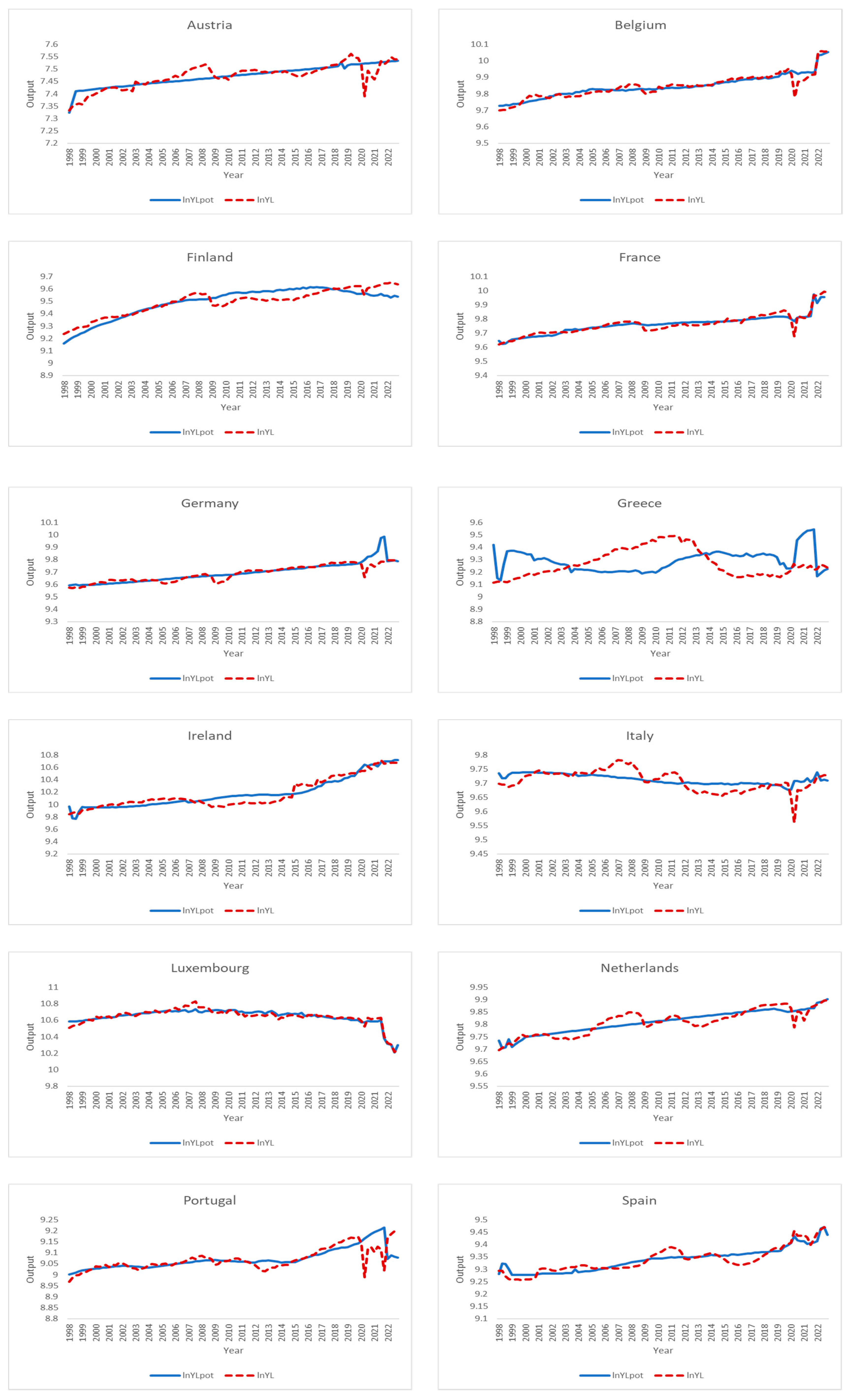
Figure 3 depicts the natural logarithms of potential and actual output per worker for all EA-12 economies, in the period 1998–2022.

There are several impressive factors revealed in Figure 3. Italy has seen a steady decline in its potential output per worker since the country adopted the Euro, a situation that was not changed with the 2008 GFC. Greece recorded a decline in potential output per worker and, after 2010, an increase, followed by stagnation. All other countries recorded an increase in their potential output per worker, with Ireland and Portugal improving in their increase after implementation of quantitative easing by the ECB, in 2015.

As expected, actual output per worker was more volatile than potential output per worker, with the output gap per worker being sometimes positive and other times negative. Costa et al. (2021) found that the amplitude of the business cycle and the persistence of shocks were higher in the Portuguese economy than in the German one. We obtained the same result regarding Germany and Portugal, but we cannot say that the amplitude of the business cycle and the persistence of shocks were necessarily higher in EA-12 MS that are net recipients of the EU budget than they were in EA-12 MS that are net contributors of the EU budget. Germany and France, the two larger economies of the EA-12, seem to have a business cycle with lower amplitude and persistence of the shocks than the other EA-12 MS, while the opposite occurs with Greece, followed by Italy. In Portugal, it is noteworthy that austerity pursued in the EA as a response to the 2008 GFC had a higher impact as a negative shock than the 2008 GFC itself.

Still looking at actual output per worker, the impacts of the COVID-19 pandemic are visible, proving to be more severe than the 2008 GFC in most EA-12 MS. MS relying heavily on the tourism sector, such as Portugal, were severely hit by the COVID-19 pandemic.

5.2. SURE Model Estimation Results, Partial Output Elasticities, and Allen Input Substitution Elasticities

Equations (3) and (4) were simultaneously estimated for all the EA-12 economies using the SURE model.

Table 1. Regression results (EA-12 MS net contributors of the EU budget in the period).

	Germany	Netherlands	France	Italy	Austria	Finland	Ireland
lnKL	0.533 ****	0.109 ****	0.515	0.157 ****	0.304 ****	0.5 ****	0.252 ****
lnHL	0.210 ****	0.299 ***	0.023 ****	0.174	0.559 ****	0.485 ****	0.151 ****
t	−2.82 × 10−5 ****	−4.27 × 105 ****	−1.63 × 104 ****	−8.8 × 105 ***	−2.18 × 10−6 ****	−3.39 × 10−4 ****	2 × 10−4 ****
lnKL2	9.87 × 10−4 ****	0.029 ****	0.0174 ****	0.033 ****	4.59 × 10−3 ****	0.006 ****	0.017 ****
lnHL2	0.001 *	−0.052 ***	0.003	0.037	0.006 ****	0.001 ****	0.452 ****
lnKLlnHL	0.783 ****	0.008	0.002 ***	−0.001	0.013 ****	−4.25 × 10−4 ****	0.232 ****
constant	0.079 ****	−0.001	0.125 ****	0.007 ****	0.001	0.419 ****	−0.023 ****
RMSE	0.000966	0.001551	0.0047342	0.0040004	0.0000133	0.003713	0.0023355
R2	0.9344	0.9082	0.9466	0.9775	0.9015	0.9211	0.9865
OGln-1	6.17 × 10−7 ****	−5.30 × 10−6 ***	−9.76 × 10−6 ***	−6.35 × 10−6	−2.16 × 10−4 ****	−3.42 × 10−6	−8.21 × 10−6 ****
OGln-2	4.96 × 10−6	5.24 × 10−6	1.04 × 10−5 ****	−3.31 × 10−6	7.66 × 10−5	1.5 × 10−6	6.60 × 10−6 ***
RMSE	0.016183	0.013354	0.0295258	0.0168496	0.0179341	0.014802	0.032909
R2	0.164	0.0862	0.0616	0.0501	0.1643	0.0159	0.079

Source: own work. In first differences, the estimation of each model equation for each MS was based on 98 observations. Levels of significance: **** 1%, *** 5%, ** 10%, and * 15%.

and

Table 2. Regression results (EA-12 MS net recipients of the EU budget in the period).

	Luxembourg	Belgium	Spain	Portugal	Greece
lnKL	0.111 ****	0.618 ****	0.724 ****	0.478 ****	0.108 **
lnHL	0.026 ****	0.521 ****	0.27	0.191 ***	0.14
t	−3.39 × 10−4 ***	1.41 × 10−4 ****	2.17 × 10−4 ****	−2.18 × 10−4 ****	3.13 × 10−5 *
lnKL2	0.031 ****	−0.007	−0.1 ****	0.001 *	0.007 ***
lnHL2	0.004 ****	−0.182 ****	−0.063	0.002	−0.007 ****
lnKLlnHL	0.045 ****	0.009 ****	0.009	0.003 ***	0.004
constant	−0.005 ****	−0.020 ****	−0.023 ****	0.019 ****	−0.007 ****
RMSE	0.0014919	0.0014278	0.004759	0.00599	0.004887
R2	0.9069	0.9834	0.8649	0.919	0.9734
OGln-1	2.88 × 10−9	1.31 × 10−6 **	1.63 × 10−5 ***	−2.83 × 10−5 ****	7.70 × 10−6 ***
OGln-2	3.4 × 10−8	−1.24 × 10−6	−2.24 × 10−5 ****	−1.75 × 10−5 *	−7.32 × 10−6 ****
RMSE	0.2811911	0.0229447	0.009876	0.021722	0.004887
R2	0.0018	0.0955	0.0235	0.0649	0.0328

Source: own work. In first differences, the estimation of each model equation for each MS was based on 98 observations. Levels of significance: **** 1%, *** 5%, ** 10%, and * 15%.

show the estimation results.

The explanatory power of the estimated SURE model in first differences was high. Most of the coefficients were also significant in the second equation (which corroborates the existence of hysteresis). The latter coefficients are elasticities that indicate the percentage increase in potential output when the lagging ratios of actual output to potential output increase by one percent. It is important to note that these lagging ratios can be either less than or greater than one, depending on the MS, which may explain the different signs of the coefficients found in the various MS and lagging periods.

With the empirical approach employed in this research, it is feasible to compute other elasticities mentioned in the literature (see Tervala 2021).

Table 3. Partial potential output and Allen input substitution elasticities.

	εk	εh	σhk
Net contributors	0.52	0.36	0.46
Germany	0.56	0.37	0.69
Netherlands	0.47	0.33	0.16
France	0.66	0.22	0.63
Italy	0.53	0.20	0.22
Austria	0.41	0.52	0.19
Finland	0.57	0.48	0.67
Ireland	0.44	0.38	0.66
Net recipients (*)	0.47	0.32	0.56
Luxembourg	0.56	0.61	0.13
Belgium	0.54	0.42	0.83
Spain	0.62	0.44	0.86
Portugal	0.49	0.23	0.17
Greece	0.21	0.18	0.38

Source: own work. (*) Excluding Luxembourg.

illustrates the partial potential output and Allen input substitution elasticities for the period 1998–2022, evaluated at the sample mean. Regarding the estimated results, it is worth noting that Luxembourg stands out as an outlier. Consequently, we present the results for this country separately, excluding it from the calculation of average net recipients in Table 3 and throughout the article, as well as from the discussion of the results.

The partial potential output with respect to physical (human) capital elasticity, ε_k (ε_h), quantifies how responsive the potential output is to variations in the trend of physical (human) capital. The Allen elasticity of substitution between trends of physical and human capital (σ_hk) quantifies the extent to which these two production factors can be substituted for or complement each other. EA-12 MS net contributors and net recipients of the EU budget had, on average, similar elasticities. Except for Austria, ε_k was always higher than ε_h. Concerning σ_hk, it was positive in all EA-12 economies, showing substitution between physical capital and human capital in all of them.

Regarding physical capital, France stood out with the highest positive ε_k (0.66), indicating that a 1% increase in the trend of physical capital resulted in an increase in potential output of 0.66%. In contrast, Greece exhibited the lowest ε_k value (0.21), indicating that a 1% increase in the trend of physical capital led to an increase in potential output of 0.21%. These findings highlight the substantial variation in the impact of the trend of physical capital on potential output among the EA-12 MS, even within those that are net contributors and net recipients of the EU budget.

Concerning human capital, Austria boasted the highest ε_h value (0.52), signifying that a 1% increase in the trend of human capital resulted in a 0.52% increase in potential output. In stark contrast, Greece exhibited the lowest ε_h (0.18), suggesting that a 1% increase in the trend of human capital led to a 0.18% increase in potential output. These findings echo the significant variation in the impact of the trend of human capital on potential output among EA-12 MS, even within net contributors and net recipients of the EU budget.

When it comes to the substitution between the trends of physical and human capital, Germany exhibited the highest positive value of σ_hk (0.69), suggesting a relatively strong likelihood of substitution between these two factors. Conversely, the Netherlands exhibited the lowest value of σ_hk (0.16), suggesting weaker possibilities of substitution between physical and human capital compared to Germany. These findings underscore that the degree of substitution between trends of physical and human capital varies significantly across EA-12 economies, even within MS that are net contributors and those that are net recipients of the EU budget.

In summary, the elasticity values revealed diverse responsiveness in potential output to changes in trend input factors across the EA-12 MS. Interestingly, this heterogeneity persisted even within MS net contributors and net recipients of the EU budget. The varying magnitudes of these elasticities underscore the distinct effects of trends of physical and human capital on potential output, as well as the degree of substitution between these production factors within the EA-12 MS.

5.3. Output Gap and Returns to Scale Rankings

Table 4. Rankings based on the output gap and returns to scale.

Rank	MS	Output Gap	MS	Returns to Scale
1	Finland	0.24%	Luxembourg	1.17
2	France	0.12%	Spain	1.06
3	Spain	0.05%	Finland	1.05
4	Luxembourg	0.02%	Belgium	0.96
5	Belgium	0.00%	Germany	0.93
6	Austria	0.00%	Austria	0.93
7	Portugal	−0.05%	France	0.88
8	Netherlands	−0.07%	Ireland	0.82
9	Ireland	−0.10%	Netherlands	0.80
10	Italy	−0.36%	Italy	0.73
11	Greece	−0.45%	Portugal	0.72
12	Germany	−0.65%	Greece	0.39

Source: own work.

presents two rankings of the EA-12 MS, respectively, based on the output gap and returns to scale. The output gap and returns to scale for each MS are average values computed for the entire period (1998–2022).

Once again, the heterogeneity of values goes beyond the division between MS net contributors and net recipients of the EU budget. The output gap measures the difference between actual output per worker and potential output per worker as a percentage of the latter, reflecting the level of demand observed in relation to installed capacity, while returns to scale assess changes in potential output in response to proportional changes in trend inputs. In terms of the output gap, Finland led the ranking, with a positive value of 0.24%. Portugal, the Netherlands, Ireland, Italy, Greece, and Germany presented negative output gaps. Concerning these MS, Germany’s leadership in terms of output gap magnitude can be explained by the fact that the country relies heavily on external demand. In terms of returns to scale, Spain stood out with the highest value (1.06) and Greece with the lowest (0.39), with Spain (1.06) and Finland (1.05) presenting increasing returns to scale.

5.4. The Decomposition of Growth

Table 5. The decomposition of growth in actual output per worker of EA-12 MS net contributors of the EU budget (quarterly % rate).

	Group Average	Germany	Netherlands	France	Italy	Austria	Finland	Ireland
Growth in potential output per worker	0.30	0.22	0.17	0.36	−0.03	0.21	0.39	0.80
1. TFP Change	0.77	0.13	0.05	0.37	0.28	0.09	2.66	1.83
- Technical change	0.85	0.33	0.14	0.44	0.42	0.14	2.50	1.98
- Scale efficiency change	−0.08	−0.20	−0.09	−0.07	−0.14	−0.05	0.16	−0.15
2. TFA Change	1.35	3.24	0.45	0.55	0.53	0.67	3.16	0.84
- Physical capital change	1.24	3.21	0.36	0.45	0.44	0.59	3.08	0.54
- Human capital change	0.11	0.03	0.10	0.09	0.09	0.08	0.08	0.30
3. Random Shocks	−1.82	−3.15	−0.34	−0.56	−0.83	−0.54	−5.43	−1.87
- Explained by lagging output gaps	0.00	0.00	0.00	0.00	0.00	0.00	0.00	0.00
- Unexplained	−1.82	−3.15	−0.34	−0.56	−0.83	−0.54	−5.43	−1.86
Growth in actual output per worker	0.33	0.23	0.21	0.36	0.04	0.23	0.42	0.80
Output gap changes	0.02	0.01	0.04	0.00	0.07	0.02	0.03	0.00

Source: own work.

and

Table 6. The decomposition of growth in actual output per worker of EA-12 MS net recipients of the EU budget (quarterly % rate).

	Group Average (*)	Luxembourg	Belgium	Spain	Portugal	Greece
Growth in potential output per worker	0.14	−0.25	0.34	0.17	0.09	−0.05
1. TFP Change	−0.33	12.34	0.45	−1.27	0.38	−0.86
- Technical change	−0.19	2.50	0.56	−1.43	0.77	−0.64
- Scale efficiency change	−0.14	9.84	−0.11	0.16	−0.39	−0.22
2. TFA Change	1.84	56.25	2.91	2.68	1.41	0.36
- Physical capital change	1.69	56.10	2.87	2.48	1.24	0.15
- Human capital change	0.16	0.15	0.04	0.21	0.17	0.20
3. Random Shocks	−1.38	−68.84	−3.03	−1.25	−1.70	0.46
- Explained by lagging output gaps	0.00	0.00	0.00	0.00	0.00	0.00
- Unexplained	−1.38	−68.84	−3.03	−1.25	−1.70	0.46
Growth in actual output per worker	0.21	−0.20	0.39	0.18	0.14	0.14
Output gap changes	0.08	0.05	0.06	0.01	0.05	0.19

Source: own work. (*) Excluding Luxembourg.

show the decomposition of growth in potential and actual output per worker by MS and groups of MS. The average values were computed for the period 1998–2022.

The average quarterly growth rates of potential and actual output per worker exhibited significant variations among EA-12 MS, which go beyond the division between net contributors and net recipients of the EU budget. Nonetheless, as a group and on average, EA-12 MS net contributors of the EU budget have grown more in terms of potential output per worker (0.30%) than EA-12 MS net recipients in the period (0.14%), with both groups of countries having small output gap changes (0.02% and 0.08%, respectively). Ireland, Finland, and France are the MS with the highest growth rates, while Greece, Portugal, and Spain are the MS with the lowest growth rates. In Greece, the average quarterly growth rate of potential output per worker was negative in the period (−0.05%).

Looking at the decomposition of potential output growth by EA-12 MS, net contributors of the EU budget showed a positive TFP change (1.84%), while for net recipients of the EU budget, the TFP change was negative (−0.33%). This is mainly explained by technical change (0.85% and −0.19%, respectively). The scale effects were negative for both groups of countries (−0.08% and −0.14%, respectively).

TFA change was positive for both groups of economies, being smaller for MS net contributors of the EU budget than for MS net recipients (1.35% and 1.84%, respectively), with less accumulation of both the trend of physical capital (1.24% and 1.69%, respectively) and the trend of human capital (0.11% and 0.16%, respectively).

Finally, the random shocks component, on average, negatively affected the growth in potential output of EA-12 MS net contributors and net recipients of the EU budget (−1.82% and −1.38%, respectively). It is important in magnitude, but barely explained by lagging output gaps.

6. Conclusions

The objectives of this article were: (i) to analyze the growth of potential output per worker, as well as the changes in the output gap per worker in the EA-12 MS net contributors and net recipients of the EU budget, and (ii) to explore the existence of hysteresis or long-lasting effects of shocks within the specified MS. To this end, we employed an innovative empirical approach that integrates the analysis of both growth and cycles.

A SURE model was employed to estimate a translog production frontier and to analyze the impacts of lagging output gaps on potential output per worker for each of the EA-12 MS. This was achieved using quarterly data, filtered through the Kalman filter, over the period spanning from 1998 to 2022. The model was estimated in first differences.

The results confirmed the existence of hysteresis, but the impact of a lagging output gap on potential output appeared to be minimal. Additionally, they revealed a pronounced degree of heterogeneity across the EA-12 economies. This heterogeneity transcends the binary classification of MS net contributors and net recipients of the EU budget, manifesting itself within each of these two groups in terms of the business cycle, potential output per worker, potential output partial elasticities, Allen input substitution elasticities, output gaps, returns scale, the decomposition of growth, and hysteresis.

Despite the heterogeneity across EA-12 MS within each of the two groups, TFP change, specifically technical change, played a more prominent role in explaining potential output per worker growth in EA-12 MS that are net contributors to the EU budget than in MS that are net recipients. Conversely, TFA change, particularly physical capital accumulation, was more influential in explaining potential output per worker growth in EA-12 MS that are net recipients of the EU budget than in MS that are net contributors. These specific results seem to reflect the budgetary stance of each MS group and the utilization of European funds by net recipients of the EU budget.

The observed heterogeneity across the EA-12 MS also raised important questions regarding the effectiveness of the one-size-fits-all monetary policy approach adopted by the ECB. A singular monetary policy is hardly adequate to address the varying needs and challenges faced by each MS, as their economies possess different structural characteristics and respond differently to the same monetary measures. Consequently, there arises a need for the ECB to adopt a more tailored approach—one that recognizes and accommodates the unique economic circumstances of individual EA MS. Such a customized approach may require not only the use of unconventional monetary policy, but also the incorporation of fiscal policy within the context of a complete EA.

This research has limitations. The results may be sensitive to the Kalman filter employed. For sensitivity analysis regarding the filter, an alternative filter that is widely used in the literature, despite its limitations, is the Hodrick–Prescott (HP) filter.

The choice of functional form for the production frontier can also influence the results. While the translog functional form is widely used in frontier literature due to its flexibility, it necessitates estimating a substantial number of parameters. This requirement is particularly challenging with a limited sample size. Since our results point toward the substitution of inputs, an alternative functional form worth exploring is the Constant Elasticity of Substitution (CES) production function, which is widely used in the production function literature. It offers some flexibility while potentially overcoming the parameter estimation issue.

Similar to common practice in the production function literature, we can enhance our estimation of each MS production frontier within the SURE framework by incorporating additional equations and/or imposing specific restrictions that provide more information for model estimation.

Finally, our results may be sensitive to both the sample size and the number of considered MS. Although the MS of the EU are not necessarily part of the EA, the single market connects them. To enhance our analysis, we could extend the time period from 1995 to 2022, including all EA-12 MS as well as Denmark and Sweden. The latter are two MS that did not adopt the Euro.

References

1. Aguiar, Diana, Leonardo Costa, and Elvira Silva. 2017. An Attempt to Explain Differences in Economic Growth: A Sochastic Frontier Approach. Bulletin of Economic Research 69: E42–65. [Google Scholar] [CrossRef]
2. Atkinson, Tim, John Dolmas, Chris Koch, Eric F. Koenig, Karen Mertens, Andrew Murphy, and Kevin M. Yi. 2020. Mobility and Engagement following the SARS-CoV-2 Outbreak. Dallas: Federal Reserve Bank of Dallas. [Google Scholar]
3. Avouyi-Dovi, Stéphane, and Jean-Guillaume Sahuc. 2016. On the sources of macroeconomic stability in the euro area. European Economic Review 83: 40–63. [Google Scholar]
4. Baldwin, Richard, and Francesco Giavazzi. 2015. The Eurozone Crisis—A Consensus View of the Causes and a Few Possible Solution. London: CEPR Press. [Google Scholar] [CrossRef]
5. Ball, Laurence M. 2009. Hysteresis in Unemployment: Old and New Evidence (No. w14818). Cambridge: National Bureau of Economic Research. [Google Scholar]
6. Ball, Laurence M. 2014. Long-term damage from the great recession in OECD countries. European Journal of Economics and Economic Policies: Intervention 11: 149–60. [Google Scholar] [CrossRef]
7. Ball, Laurence M., and Janine Onken. 2022. Hysteresis in unemployment: Evidence from OECD estimates of the natural rate. International Finance 25: 268–84. [Google Scholar] [CrossRef]
8. Barro, Robert J., and José W. Lee. 2013. A new data set of educational attainment in the world, 1950–2010. Journal of Development Economics 104: 184–98. [Google Scholar] [CrossRef]
9. Barro, Robert J., and JoséF. Ursúa. 2008. Macroeconomic Crises Since 1870. Brookings Papers on Economic Activity 2008: 255–335. Available online: https://www.jstor.org/stable/27561619 (accessed on 25 February 2024). [CrossRef]
10. Barua, Saurabh. 2020. Understanding Coronanomics: The Economic Implications of the Coronavirus (COVID-19) Pandemic. SSRN Electronic Journal 1: 1–44. [Google Scholar] [CrossRef]
11. Blanchard, Olivier. 2016. The Phillips curve: Back to the ‘60s? American Economic Review: Papers & Proceedings 106: 31–34. [Google Scholar] [CrossRef]
12. Blanchard, Olivier, and Jordi Galí. 2007. Real wage rigidities and the new Keynesian model. Journal of Money, Credit and Banking 39: 35–65. [Google Scholar] [CrossRef]
13. Blanchard, Olivier J., and Danny Quah. 1989. The dynamic effects of aggregate demand and supply disturbances: Another look. The American Economic Review 79: 655–73. [Google Scholar] [CrossRef]
14. Blanchard, Olivier J., and Lawrence H. Summers. 1986. Hysteresis in unemployment. In Economic Models of Trade Unions. Dordrecht: Springer, pp. 235–42. [Google Scholar]
15. Blanchard, Olivier, Enrica Cerutti, and Lawrence Summers. 2015. Inflation and Activity—Two Explorations and their Monetary Policy Implications. IMF Working Papers. Washington, DC: International Monetary Fund, vol. 15, p. 1. [Google Scholar] [CrossRef]
16. Campbell, John Y., and N. Gregory Mankiw. 1987. Permanent and Transitory Components in Macroeconomic Fluctuations. American Economic Review 77: 111–17. [Google Scholar]
17. Carlsson-Szlezak, Phillip, Martin Reeves, and Paul Wartz. 2020. What Coronavirus Could Mean for the Global Economy. Available online: https://hbr.org/2020/03/what-coronavirus-could-mean-for-the-global-economy (accessed on 25 February 2024).
18. Cerra, Valerie, and Sweta C. Saxena. 2008. Growth dynamics: The myth of economic recovery. American Economic Review 98: 439–57. [Google Scholar] [CrossRef]
19. Cerra, Valerie, and Sweta Saxena. 2017. Booms, Crises, and Recoveries: A New Paradigm of the Business Cycle and Its Policy Implications. IMF Working Papers. Washington, DC: International Monetary Fund, vol. 17, p. 1. [Google Scholar] [CrossRef]
20. Cerra, Valerie, Antonio Fatás, and Sweta C. Saxena. 2023. Hysteresis and business cycles. Journal of Economic Literature 61: 181–225. [Google Scholar] [CrossRef]
21. Christensen, Laurits R., Dale W. Jorgenson, and Lawrence J. Lau. 1973. Transcendental Logarithmic Production Frontiers. The Review of Economics and Statistics 55: 28–45. [Google Scholar] [CrossRef]
22. Claessens, Stjin, and M. Ayhan Kose. 2018. Frontiers of Macrofinancial Linkages. BIS Paper. Basel: Bank for International Settlements. [Google Scholar]
23. Clarida, Richard, Jordi Galı, and Mark Gertler. 1998. Monetary policy rules in practice: Some international evidence. European Economic Review 42: 1033–67. [Google Scholar] [CrossRef]
24. Costa, Leonardo, Nuno O. Martins, and Francisca Guedes de Oliveira. 2016. Portugal’s bailout and the crisis of the European Union from a capability perspective. Cambridge Journal of Economics 40: 1479–96. [Google Scholar] [CrossRef]
25. Costa, Leonardo, Francisca. Guedes de Oliveira, Alexandra Leitão, and João Paredes. 2021. Business cycles and trends in Germany and Portugal: Macroeconomic policy implications in the Euro Area. European Planning Studies 29: 654–80. [Google Scholar] [CrossRef]
26. De Grauwe, Paul. 2012. A fragile Eurozone in search of a better governance. Economic and Social Review 43: 1–30. [Google Scholar] [CrossRef]
27. Dosi, Giovanni, Mauro C. Pereira, Andrea Roventini, and Maria E. Virgillito. 2018. Causes and consequences of hysteresis: Agregate demand, productivity, and employment. Industrial and Corporate Change 27: 1015–44. [Google Scholar] [CrossRef]
28. Fernandes, Nuno. 2020. Economic Effects of Coronavirus Outbreak (COVID-19) on the World Economy. IESE Business School Working Paper No. WP-1240-E. Barcelona: IESE Business School. [Google Scholar] [CrossRef]
29. Fornaro, Luca, and Martin Wolf. 2020. COVID-19 Coronavirus and Macroeconomic Policy. Health Economics eJournal 2020: 1–12. Available online: https://ssrn.com/abstract=3560337 (accessed on 25 February 2024).
30. Ghosh, Jayati. 2022. Dealing with Inflation, Really. Berlin: Social Europe. [Google Scholar]
31. Goodfriend, Marvin, and Robert G. King. 1997. The New Neoclassical Synthesis and the Role of Monetary Policy. NBER Macroeconomics Annual 12: 231–283. [Google Scholar] [CrossRef]
32. Gordon, Robert J. 1984. Supply Shocks and Monetary Policy Revisited. The American Economic Review 74: 38–43. Available online: https://www.jstor.org/stable/1816327 (accessed on 25 February 2024).
33. Guerrieri, Veronica, Lorenzoni Guido, Ludwig Straub, and Iván Werning. 2022. Macroeconomic Implications of COVID-19: Can Negative Supply Shocks Cause Demand Shortages? American Economic Review 112: 1437–74. [Google Scholar] [CrossRef]
34. Ioannides, Yannis M., and Christopher A. Pissarides. 2015. Is the Greek Crisis One of Supply or Demand? Brookings Papers on Economic Activity. Baltimore: The Johns Hopkins University Press, pp. 349–83. [Google Scholar]
35. Krugman, Paul. 2012. Revenge of the optimum currency area. NBER Macroeconomics Annual 27: 439–48. [Google Scholar] [CrossRef]
36. Kumbhakar, Subal C., and C. A. Knox Lovell. 2000. Stochastic Frontier Analysis. Cambridge: Cambridge University Press. [Google Scholar]
37. Lucas, Robert E., Jr. 2003. Macroeconomic Priorities. American Economic Review 93: 1–14. [Google Scholar] [CrossRef]
38. McKibbin, Warnick, and Roshen Fernando. 2021. The Global Macroeconomic Impacts of COVID-19: Seven Scenarios. Asian Economic Papers 20: 1–30. [Google Scholar] [CrossRef]
39. Psacharopoulos, G, and Harry A. Patrinos. 2018. Returns to investment in education: A decennial review of the global literature. Education Economics 26: 445–58. [Google Scholar] [CrossRef]
40. Romer, Paul. 2016. The Trouble with Macroeconomics. Available online: https://paulromer.net/the-trouble-with-macro/ (accessed on 25 February 2024).
41. Tervala, Juha. 2021. Hysteresis and the welfare costs of recessions. Economic Modelling 95: 136–44. [Google Scholar] [CrossRef]
42. Tervala, Juha, and Thomas Watson. 2022. Hysteresis and fiscal stimulus in a recession. Journal of International Money and Finance 124: 102614. [Google Scholar] [CrossRef]
43. Vines, David, and Samuel Wills. 2018. The rebuilding macroeconomic theory project: An analytical assessment. Oxford Review of Economic Policy 34: 1–42. [Google Scholar] [CrossRef]
44. Yellen, Janet L. 2017. Inflation, uncertainty, and monetary policy. Business Economics 52: 194–207. [Google Scholar] [CrossRef]
Figure 1. Net contributors and recipients of the EU budget (GDP percentage average 1998–2022). Source: own work based on the European Commission’s data.
Economies 12 00084 g001
Figure 2. Current account imbalances in the EA (% of GDP, average 1998–2008). Source: own work based on the European Commission’s data.
Economies 12 00084 g002
Figure 3. Potential and actual output per MS. Source: own work.
Economies 12 00084 g003