The Timing and Strength of Inequality Concerns in the UK Public Debate: Google Trends, Elections and the Macroeconomy

Abstract

Inequality among people has several unwanted effects, in humanistic, social and economic contexts. Several studies address distributional preferences among groups, but little is known about when inequality issues are focused and when and why inequality abatement measures are brought on the political agenda. We show that during the period 2004 to 2023, inequality issues were focused during elections to the EU and UK parliament and with greatest strength during the elections to the EU parliament in May 2004 and to the UK parliament in May 2015. Periods with high unemployment and inflation cause the discussion on inequality to be followed by discussions on inequality measures. However, when the discussion of inequality is followed very closely by the discussions of abatement measures, inequality aversion becomes more strongly associated with the macroeconomic variables inflation and GDP (recessions) than with unemployment and more strongly associated with the concerns for fairness than concerns with war and crime. The results were obtained examining Google Trends and scholarly studies.

1. Introduction

Inequality (INE) among people within countries and worldwide has been hypothesized to cause political instability, e.g., Roe and Siegel (2011), decrease economic growth, e.g., Michalek and Vybostok (2019), and contrast with what people regard as morally right, Rözer et al. (2022). Peoples’ perception of inequality of pay has also been found to be strongly connected to their political standpoint (Bratanova et al. 2016; Fisman et al. 2017; Sandnes et al. 2023). However, Hoy et al. (2024, data from Australia) show that the opinions of right-leaning voters change when misconceptions are corrected. A popular survey of relations between inequality and population “spirit” is given in Wilkinson and Pickett (2010, data sources pp. 280–83). Three sets of questions with regard inequality can be distinguished: A first set addresses the factors that contribute to increasing or decreasing inequality. A second set addresses which of these factors are the result of economic policy to stabilize the economy, and which factors can be managed directly to address inequality, e.g., Malla and Pathranarakul (2022). The third set addresses the type of inequality concerns expressed by low-, middle- and high-income populations. Most of the current literature on inequality appears to address the concerns expressed by the low-income population.

Recently, Google Trends have been used to identify people’s sentiments in the public conversation about important issues. For example, Timoneda and Wibbels (2022, pp. 3–6) discussed the use of Google Trends and examined the frequency of “protests” using Google Trends. Connor et al. (2019) searched for links between “inequality” and “racial-bias” but found no conclusive evidence for such a link. Here, we examine if the two issues, “inequality” (INE) and “inequality measures” (IMEs), were related to particular events or macroeconomic economic states in the United Kingdom (UK). The UK was chosen because it ranks among the highest in Europe in terms of income inequality (Berisha et al. 2021), and Filippin and Nunziata (2019, p. 116) include the UK among the high-inequality cluster of European states.

We developed three hypotheses.

Hypotheses. We hypothesized that

Hypothesis 1 (H1).

Conversations about INE and measures to reduce inequality, IME, would be particularly strong around elections to the UK and the European union (EU) parliaments. The raationale is that when inequality becomes a focused issue in the public conversation, the need for measures to abate inequality will be stronger and therefore follow in strength in the conversation. For example, Fisman et al. (2017) argues that redistribution versus anticipated GDP growth was an important issue during the US presidential election in 2012. We evaluate the hypothesis by identifying time windows in Google Trends series where frequencies are larger than one half the series’ average frequency; in the following, these are denoted by INE+ and IME+. The technique of identifying windows in time series where values that are higher and lower than the average value is common in climate research; e.g., Gong et al. (2020).

Second, we hypothesized that

Hypothesis 2 (H2).

INE would be leading IME during unfavorable economic conditions. Such periods could be periods with high unemployment (UE), high inflation (INF) and low central bank interest rate (CBI). CBI is low when the economy is underperforming. We evaluate this hypothesis by (i) applying a high-resolution lead-lag method (HRLL) to paired Google time series and (ii) embedding the LL relations in a principal component analysis (PCA) “map” of the UK economy. This allows us to identify which economic conditions are associated with a leading relation for INE to IME, that is, from inequality discussions to inequality abatement measures.

Third, we hypothesized that

Hypothesis 3 (H3).

A major reason for conflicts related to inequality would be “fairness” issues. We evaluated this hypothesis by comparing Google Trends series for “inequality” with Trends series for “fairness”. If the two series should correlate, fairness is an important attribute of inequality.

Since the political events associated with a parliament election last for a relatively short period, whereas economic changes typically last for the length of economic business cycle times, e.g., 4–8 years (Burns and Mitchell 1946), we disentangle the time series into a high-frequency, rapid component and a low-frequency, slow component.

We find that inequality in the UK is in focus during parliament elections, and during periods with recessions and inflations, more than with periods of unemployment. Inequality is more strongly associated with fairness than with crime and war.

The present study distinguishes itself from most other studies in that it identifies time windows during the economic and social development of a single country, the UK, whereas most other studies find patterns in inequality by studying and comparing inequality among several countries. We use a high-resolution lead-lag method (HRLL) that allows us to strengthen the causal interferences over what correlation alone would support. HRLLs are calculated over short time periods (3 months and 9 months are sufficient to establish significance). Furthermore, we add context to our results by making a PCA score plot for the UK economy from 2004 to 2023 based on five macroeconomic variables.

The rest of the manuscript is organized as follows. Section 2 presents the time series used. Section 3 describes the methods, with emphasis on a high-resolution lead-lag (HRLL) method. Section 4 shows the results, and Section 5 discusses the results. Section 6 presents concluding remarks.

2. Data

We used Google Trends https://trends.google.com/trends/?geo=NO, accessed on 5 January 2024. From that database, we retrieved time series for the frequency of the terms “inequality”, “poor” and “rich” for the period 2004 to 2024. We used the colloquial terms “poor” and “rich” instead of low- and high-income people because the second set of terms did not have enough data to construct meaningful time series. We retrieved time series for “conflict”, “political conflict” and “inequality measures” to express possible results of inequality on conflicts and abatement measures. We used the expression “Inequality measures” despite its relatively low overall scores because we then could examine if “inequality” would lead to the discussion of “inequality measures”. We also tried several other expressions for inequality measures, but none yielded enough data to construct meaningful time series. To put our results into an economic context for the UK, we used data on unemployment (UE), monetary supply (M1), inflation (INF) and industrial production (IP). The data were extracted from St. Louis Federal Reserve in 5 January 2024 (https://fred.stlouisfed.org/). Data for UK and EU parliament elections were downloaded from official governmental websites. There were eight election dates: October 2004 (EU election), May 2005 (UK election), June 2009 (EU-election) 2010 May (UK election), May 2015 (UK election), June 2017 (UK election), May 2019 (EU election), December 2019 (UK election). The UK left the EU on 31 January 2020. We retrieved an index for inequality, the Gini’s index from https://fred.stlouisfed.org/series/SIPOVGINIGBR and from https://www.statista.com/statistics/872472/gini-index-of-the-united-kingdom/, the latter to find the most recent scores. Both data sources were retrieved on 5 January 2024. The Gini index is an economic equality score calculated for all countries in the world by the World Bank (https://data.worldbank.org/indicator/SI.POV.GINI, accessed on 5 January 2024). Data for concerns related to inequality were retrieved from Google Trends, Google Scholar and Web of Science.

3. Methodology

In this section, we first disentangle the Google Trends time series into short-term and long-term components based on power spectral density (PSD) results for the Google series. We then explain how the series are detrended and smoothed to extract the features of interest. Thereafter we explain briefly the high-resolution lead-lag HRLL method used in the study, cycle periods (CP) and phase shifts (PS). Fourth, we briefly explain how we use some algorithms that are common in several statistical software packages.

3.1. Data Preprocessing

We disentangled the time series by identifying time series’ components using LOESS smoothing. The LOESS smoothing algorithm has two parameters. The parameter (f) is the fraction of the time series that is used as a moving window, and the parameter (p) is the order of the polynomial equation used to interpolate the series. Because we always use p = 2, we use the nomenclature LOESS(f) to identify the smoothing degree in the rest of the manuscript. We LOESS(0.4)-smoothed the raw time series to identify the low-frequency time series and subtracted the low-frequency time series from the raw time series to identify the high-frequency time series. To remove high-frequency noise from the high-frequency series, we, in addition, used LOESS(0.2) to smooth the series.

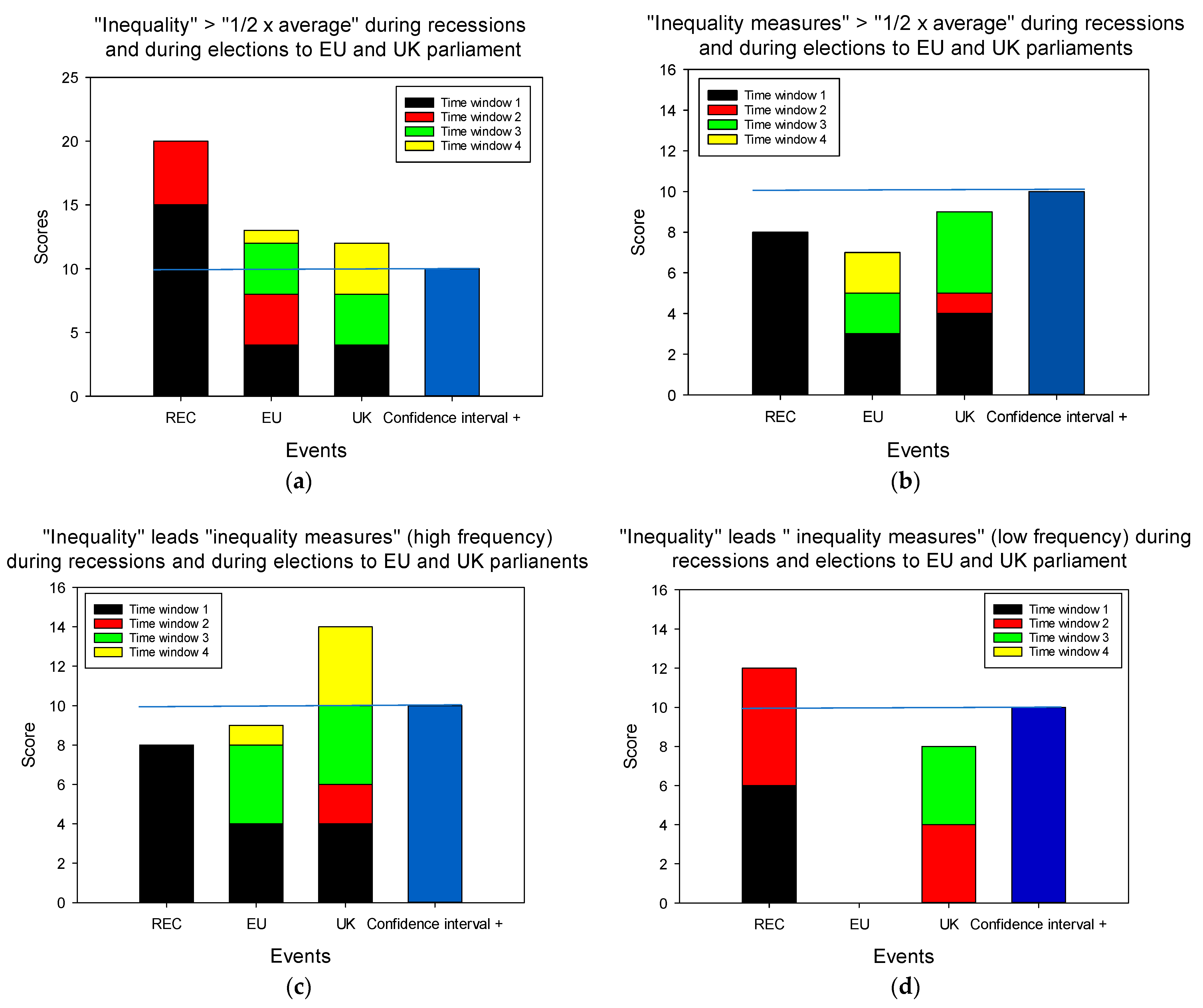
3.2. Scoring Time Series Events

To calculate scores, we identified the number of months during the two recessions and during the eight elections where (i) “inequality” and (ii) “inequality measures” showed high frequency and (iii) where “inequality” was leading “inequality measures”. Recessions lasted 16 and 6 months, respectively, and the election periods were defined as 2 months before and 1 month after the election month. This is the same time window as Timoneda and Wibbels (2022) use before and after a “protest” month.

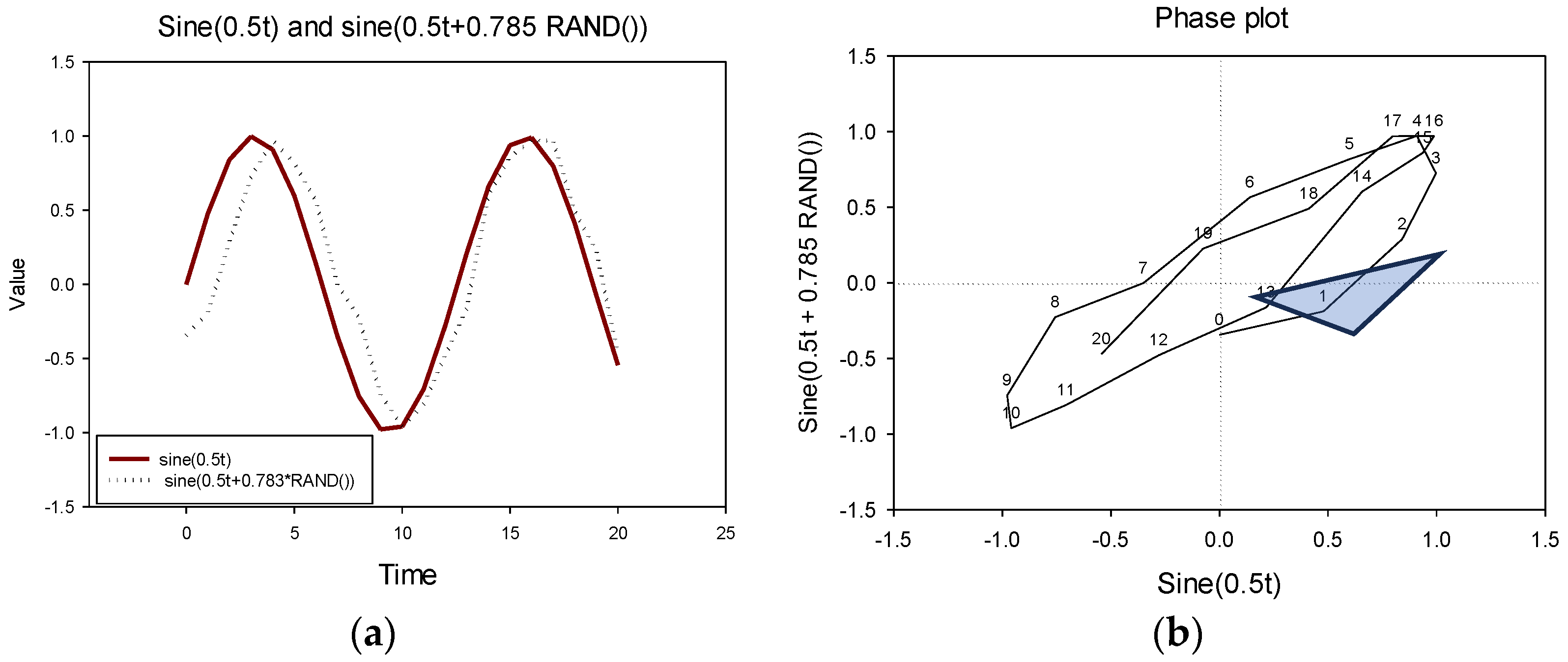
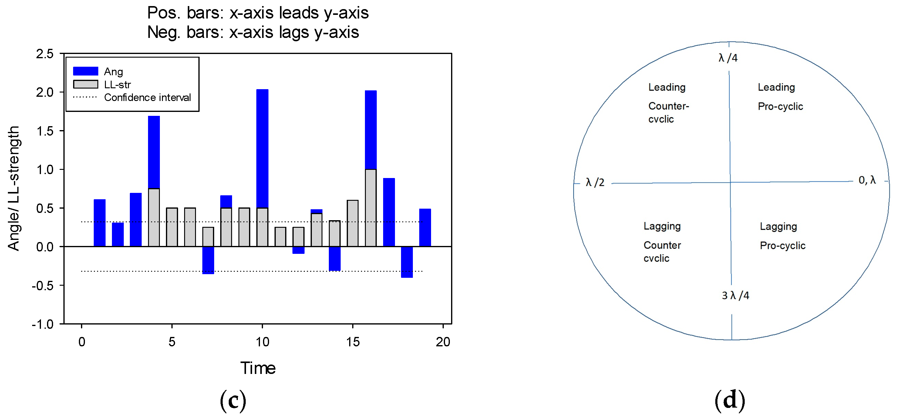
3.3. Lead-Lag Analysis

We use the high-resolution lead-lag method to examine LL relations between the time series for “inequality” and “inequality measures”. The description of the method closely follows the description given in Seip and McNown (2007). The method rests on the duality between paired time series as time series (x-axis as time, and the two series INE and IME on the y-axis) and as phase plots, with one series on the x-axis, INE, and the other series on the y-axis, IME. A persistent rotational direction in the phase plot will show that one series leads the other series in the time representation. The method allows us to select the degree of persistence of LL relations and to determine how closely the last series should follow the first series.

The method calculates an angle, θ(3), for two paired series x(t) and y(t) based on three consecutive paired observations in the phase plot for the series (x = x(t) y = y(t)). Figure 1a shows two sine series with equal cycle periods (λ), one series shifted forward relative to the other and with a small random component added. Their trajectory rotates counterclockwise (+per definition), Figure 1b. Since the LL method uses a moving window of three time steps, we can apply the method to time series that are not detrend and not stationary.

A measure of the persistence of a leading relation, the LL-strength, is defined as

$$LL\text{-}strength=(N_{+}-N_{-})/(N_{+}+N_{+})$$

where N₊ is the number of leading relations for two time series x and y, x → y, and $N_{-}$ is the number of lagging relations between the time series x ← y.

Thus, if there is a persistent positive LL relation over nine consecutive observations, the result is $N_{+}$ = 9, $N_{-}=0$ and LL = (9 − 0)/ (9 + 0) = 1. The number 9 is a tradeoff between measuring LL relations over short periods and the possibility of establishing significance. The angles, θ(3), are shown as blue bars in Figure 1c. The corresponding LL(9) values are shown as grey bars.

Confidence interval. The 95% confidence interval (CI) for the LL-strength is estimated using a Monte Carlo technique using two paired random time series. The confidence interval is found to be LL(9) = ± 0.32. Frequently, we will smooth time series, partly to avoid high-frequency noise and partly to identify cycle variabilities that are of interest, e.g., parliament election cycles. However, smoothing will increase the number of angles, θ(3), that show rotations in the same direction. Since we want to report the results for the smoothed versions, we use the term “pseudo-significant” when LL-strength <−0.32 or >0.32. Two cyclic series will either be leading or lagging in relation to each other. Visually, it is often seen as the peak of a leading series leading to a peak of the target series with less than half a common cycle period, λ/2, but the LL relation applies to all parts of the curve. If a leading series is inverted, it will be a lagging series. A leading series can both be pro-cyclic (b-coefficient positive) and counter-cyclic (b-coefficient negative) to the target series, Figure 1d.

Cycle periods, λ. When the trajectories complete one cycle in the phase plot, this corresponds to one cycle period in the time series plot. We calculate two measures of λ, one by calculating the running average λ over five consecutive time steps and one by taking the average λ of all cycle periods.

Power spectral density algorithm (PSD). The PSD algorithm identifies single cyclic series embedded in raw superimposed cyclic series. The cycle periods identified by the PSD method are compared to the cycle periods we identify with the LL method.

Lead and lag times or phase shifts (PS). The lead-lag shifts can be estimated by applying ordinary linear regression (OLR) to the time series. If they coincide perfectly, the regression coefficient, (r), is ≈ 1, and the lead-lag time, or PS, is zero. In Figure 1a, the two sine series are closely co-varying. Because both sine series were normalized to unit standard deviation, the b–coefficient (the slope) and “r” are both close to one. If the OLR gives r = −1, the two series are counter-cyclic, and the phase shift is around λ/2.

Principal component analysis (PCA). We apply PCA to five macroeconomic time series that describe the UK economy from 2004 to 2023. The PCA gives rise to two 2D plots: the score plot that shows how the economy changes over time and the loading plot that shows which of the five macroeconomic factors determine the position of the scores. For cyclic, non-Gaussian series, the position of variables in the loading plot will also reveal phase shifts between the series. The economic data were detrended to focus on events within a 3 to 5 years’ time frame.

Inequality concerns. We use the terms “fairness”, “GDP growth”, “crime” and “war” to evaluate concerns for the effects of inequality.

We use the terms in Google Trends (score range 0 to ≈50), Google Scholar (score range 500,000 to ≈4 million) and Web of Science (score range 900 to ≈300,000). To evaluate and compare the strength of the concerns for each category, we center and normalize the scores to unit standard deviation for each source. However, other terms could also be used, e.g., “female empowerment”, as in Lambert et al. (2003).

4. Results

The Google Trends time series for the 2004–2023 inequality data are shown in Figure 2a and, for conflict data, in Figure 2b. The graphs show the raw data as thin lines and LOESS(0.4)-smoothed data as thick lines. Dropdown lines indicate the beginnings of the 2008 and the 2020 recessions.

All three time series for inequality data—“inequality”, “poor” and “rich”—showed similar patterns, and the decline in frequency during the two recessions was marked (“rich” may be an exception during the 2020 recession). All three time series for conflict data—“conflict”, “political conflict” and “inequality measures”—levelled off until the 2008 recession. With the exception of “conflict”, there were few non-zero data points in the series. However, both “conflict” and “inequality measures” showed an increase in frequency around 2015. We applied the PSD algorithm to the two time series, “inequality” and “inequality measures”, and added drop lines for common cycle periods for the two series, Figure 2c. Common cycle periods for the two series occurred around 21, 43 and 64 months.

Based on these results, we LOESS-smoothed the two series so that they obtained cycle periods around 24 months (2 years) and 72 months (4 years), respectively.

Since the Gini index measures economic inequality in a country, we compared the Gini index for the UK with the Google Trends for INE for the period 2002 to 2020 (see Figure 2d). Since the two time series are measured in different units, we centered and normalized the series. There do not appear to be any relations between the two series, p = 0.17. Chroufa and Chtourou (2022) suggest that the Gini index may not be the optimal measure of inequality in a GDP growth context.

The high-frequency movements. Figure 3a,b show the results for the high-frequency time series. The LL relations suggest that the two series are leading about equally often (43% pos., 56% neg.), Figure 3b. The cycle periods were around 25 months, and the PS were around 5 to 6 months (see

Table 1. Common cycle period and phase shifts for high-frequency and low-frequency time series for the Google Trends records of “inequality” and “conflicts”.

Variables	Cycle Periods (months)	Phase Shift (months)
HF	25	5–6
LF	190 ± 136	13–22

HF = high-frequency time series, LF = low-frequency time series.

).

The low-frequency movements. Figure 3c,d shows the LOESS(0.4)-smoothed series. The LL relations suggest that INE leads IME from about year 2010, Figure 3d. The cycle periods were, on average, 190 ± 136 months, and PS were, on average, from 13 to 22 months; see Table 1.

Figure 3a,b show, for example, LL relations for an “inequality” and an “inequality measures” series. The sequence of peaks and troughs in the series in Figure 3a can be compared visually to the calculated LL relations shown in Figure 3b.

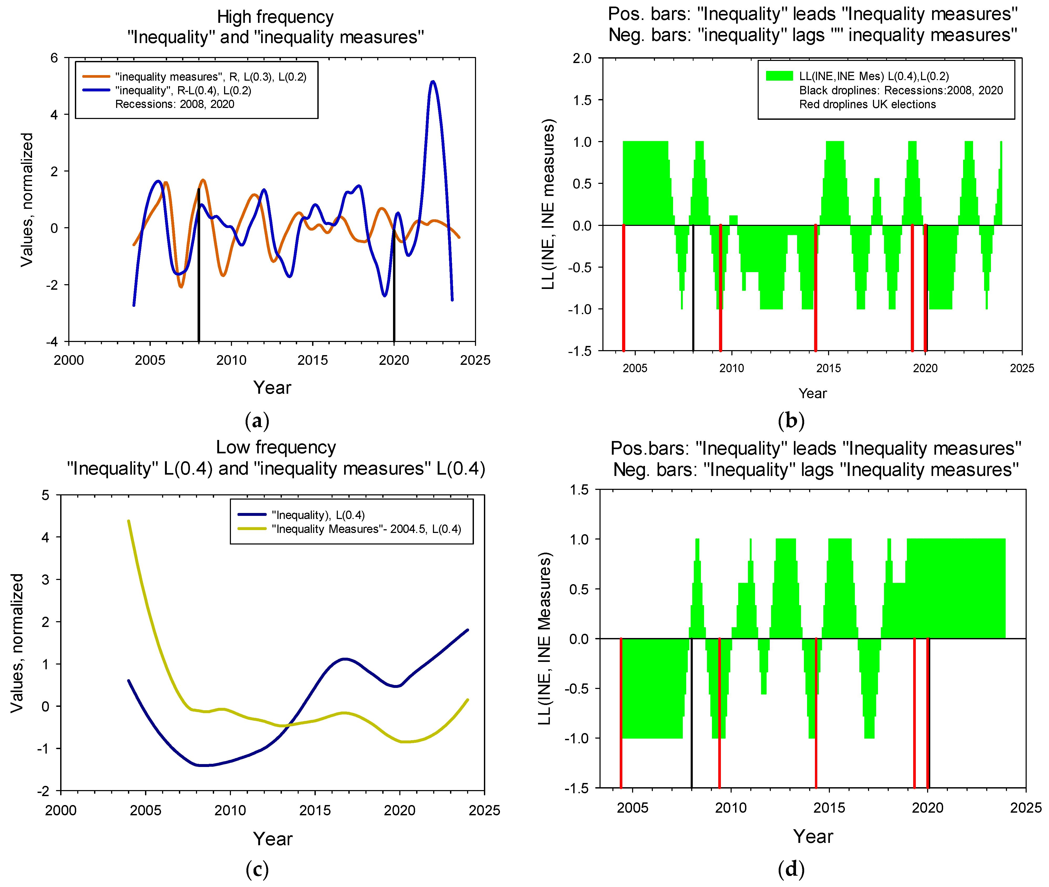
4.1. “Inequality” and “Inequality Measures” during Recessions and Parliament Elections

The result of scores during recessions and elections to EU and UK parliaments are shown in Figure 4. For each month, a value greater than half the average frequency, denoted INE+, IME+ and LL+, would give a score of “1”; otherwise, it gives a score of “0”.

There are two time windows for recessions: one starting in 2008 and lasting for 16 months and one starting in 2020 and lasting for 6 months. There are 4 months for each time window for elections to EU and UK parliaments. In the columns, the time windows are assigned different colors.

A random distribution of scores would give about two for each of the election time windows. The blue column suggests a rough estimate of the upper confidence limit for the two recessions and four elections. Figure 4 shows the scores during three “events”.

For the overall scores, the term “inequality” scores above the confidence limit during the three events: recessions, and elections to both EU and UK parliaments. IME scores below the confidence limit during all events. High-frequency INE leads IME during the UK elections, Figure 4c, and low-frequency INE leads IME during recessions, Figure 4d. It is the recessions and the UK elections that elicit the most pronounced response to inequality issues.

4.2. The UK Economy

The five time series that describe the UK economy are shown in Figure 5a.

The PCA plots for the UK economy are shown as a loading plot in Figure 5b and as score plots in Figure 5c–f. The PCA score and loading plots are interpreted as follows: The position of an observation in a score plot (in our case, the state of the UK economy at a certain year) is associated with the position of the explanatory variables in the loading plot (in our case, the values of the five macroeconomic variables). Blue dots show parliament elections and yellow dots show recessions. The loading plot shows that the time series for the five time series matches a traditional pattern for an economy.

For example, unemployment (UE) varies inversely to industrial production (IP), as it should according to Okun’s law, e.g., Maza (2022), Seip and Zhang (2022).

High-frequency results. The red lines in the left score plots in Figure 5c,e show the time windows where the high-frequency INE is a leading variable to the high-frequency IME.

The graph in Figure 5d shows results when LL relations are positive (>0; range −1 to +1), and the graph in Figure 5c shows results when LL relations are greater than 0.9, that is, the requirement for persistently tighter relations between INE and IME is strengthened.

Visually, the plot suggests that INE leads IME during periods just before, during or just after an election event, and the tighter requirement emphasizes the recession and elections during the years 2004 to 2008.

Low-frequency results. Figure 5d,f show scores where the low-frequency INE leads the low-frequency IME. The graph in Figure 5d shows the result when LL relations are positive, but for the graph in f, we have added the restriction that the lead time between INE and IME should be less than 20 months (range 0 to 100 months). The red curves in the upper right part of Figure 5d corresponds to states where INF, CBI and M1 have high values. (M1 is a technical variable expressing the amount of money in the society.)

High values of M1 and CBI suggest that the Bank of England tries to slow down the economy or reduce INF. The red curve in the upper left part corresponds to economic states where UE is high.

The graph in Figure 5f with the tighter requirement between INE and IME shows that the years from 2004 to 2008 are emphasized together with the time after the UK left the EU and the inflation period after the pandemic. The period 2011–2014 with high UE is no longer marked as an important event for discussing inequality issues. Figure 5c–f show that inequality concerns were less pronounced during the actual pandemic in 2020 than during the following inflation period up to 2023.

4.3. Inequality Concerns

Figure 6 shows two graphs that identify concerns that can be related to inequality. The first graph is based on the worldwide use of the concern terms—“fairness”, “GDP growth”, “crime” and “war”—in Google Trends, Google Scholar and the Web of Science. The second graph shows a PCA plot for the five Google Trends series: inequality and the four concern terms in the UK.

5. Discussion

We first outline the general economic history of the UK. We thereafter discuss when the frequency of inequality concerns is high. Third, we discuss the results that show when discussions on inequality are followed by discussions on inequality abatement measures, expressed by a positive lead-lag relation LL(INE, IME) value. Fourth, we examine the possible consequences of inequality, such as sentiments of unfairness in the UK population and increases in crime. Last, we discuss the use of Google Trends and the HRLL methodology.

5.1. UK Economic History 2008–2023

A rough, stylized sketch of the UK economic history can be read by comparing trajectories in the PCA “map”, Figure 5c–f, with the position of the macroeconomic variables in Figure 5b.

As trajectories in the panels of Figure 5c–f move towards the position for an acronym in panel Figure 5b, the variables represented by that acronym increase in importance for the UK economy.

Following the abrupt beginning of the recession in 2008, the economy, IP, slowed down and UE increased until 2012–2013, then UE fell, and IP grew until the COVID-19 pandemic recession in 2020. Following that recession (and the UK leaving the EU), INF rose rapidly until 2022 and then slowed down in about the same phase until the present.

It is interesting that combating the 2008 and the 2020 recessions resulted in quite different trajectories. The trajectory following the 2008 recession resulted in high UE, whereas the trajectories following the 2020 recession and pandemic resulted in high INF. However, the two recessions were handled differently using different monetary and fiscal policies.

5.2. High-Intensity Discussions of Inequality Issues

Interest in inequality, expressed as the relative frequency of the search terms “inequality”, “poor” and “rich” as reported by Google Trends, were shown in Figure 2. The term “INE” declines before the recession but increases after the recession in 2008 for 6 to 9 months. The reason may be that there is an increase in employment before a recession but a “jobless recovery” after the recession (Seip and Zhang 2022). INE is on preponderance of probability or better associated with elections to the EU and UK parliaments over short-term time spans ≈ 24 months. “Preponderance of probability” here means that “inequality” and “inequality measures” are mentioned with higher frequency than the average during all 4 months around an election. The term IME was only associated with UK elections. Our hypothesis, H1, was therefore only partly supported; both INE and IME were used more frequently than expected (random) during EU and UK elections. However, IME was used less than INE, and the terms were not used persistently during all eight election events. Inequality and its abatement measures were discussed most consistently during the EU elections in October 2004 and the UK elections in May 2005 (black EU and UK columns in Figure 4).

5.3. Lead-Lag Relations

The term INE was leading IME during elections both to the EU and the UK parliament over short time spans. By embedding the results in the “map” of the UK economy, it is seen that INE leads IME both during elections and during the recessions in 2008 and in 2020. Over the low-frequency time spans, ≈72 months, the economic “map” showed that INE was leading IME during periods with high unemployment and high inflation and during recessions. Requiring that the LL relations between INE and IME are tight, the intensity of inequality conversations around the 2008 recession and the inflation period after the COVID-19 pandemic were emphasized. Two reasons may be important: (i) there is an increased urgency to achieve inequality abatement measures, or (ii) the driving force must last for some time (>20 months), corresponding to the cutoff value for the time between high INE and IME frequencies. Thus, our hypotheses H2 was supported—a leading role for INE to IME is related to political events, that is, either to elections for the UK or the EU parliaments or to harmful economic conditions expressed by unemployment and inflation. For all terms, we tried several synonyms, but all alternatives failed to produce sufficient data.

5.4. Inequality Concerns and Inequality Abatement Measures

Inequality concerns address the effects of inequality that reduce the quality of life or the affluence of the society. Abatement measures address what policies can be enacted to reduce either “objective” inequality, (e.g., expressed by the Gini index) or “subjective” inequality. Lambert et al. (2003, p. 1073) and Davidescu et al. (2024) include macroeconomic variables (GDP per capita) but also socioeconomic variables, such as public expenditures (schools) and gender policies, to explain subjective and real inequality concerns.

5.4.1. Inequality Concerns

There are two dichotomies with respect to “inequality”. One set is if the inequality concerns relate to socioeconomic stress among the lower income individuals or if it relates to a discussion of measures to convince the rich to contribute more to the welfare system. The other set is if the rich get richer by unfair means and luck or by merit. We believe that concerns for socioeconomic stress would be dominant during recessions and during inflation events. Furthermore, discussions on stress would probably be more frequent on the internet, and discussion on how the rich could contribute more to welfare economy would probably be more frequent in reports and government hearing notes. However, in the UK, one could anticipate that discussion about contributions from the rich could be frequent during the Prime Minister period of the strongly conservative Liz Tuss from 6 September to 25 October 2022, (Tosun and Lucey 2023), but there was no pattern in the Google Trends that distinguished the period. To examine what type of concerns are most associated with inequality, we tried to combine the term “inequality” with the concern terms “fairness”, “GDP growth”, “crime” and “war”, but UK Google Trends just reported “not sufficient data”. However, time series were successfully established for the world. Figure 6a showed a comparison of the average frequency of the concern terms in Google Trends, Google Scholar and Web of Science. The first relates to public conversations, the second to scholarly research and discourses and the third to scientific publications. The concern most associated with inequality worldwide was war and, thereafter, crime. This holds for Google Trends, as well as for Google Scholar. For the Web of Science, all four concerns yielded similar results (the bars are of equal height).

For the concern terms in the UK (not paired with inequality), we obtained full series for all terms. Comparing the time series for the four terms to the series for inequality with a PCA analysis, we found that the series for fairness and GDP growth were most like the time series for inequality, Figure 6b. The overall results indicate that during elections, inequality gives reasons for discussions of abatement measures, and fairness and GDP growth are the main concerns during the discussions.

For the inequality concerns, like fairness, GDP growth, crime and war, most of the available literature gave information that was generic. The effects of inequality on economic growth were studied by Naguib (2015, p. 38 Appendix). The author examined countries that are members of the Organization for Security and Co-operation in Europe (OSCE) and found a statistically significant positive effect from inequality on GDP growth (a 1% increase in inequality gave a 1.2–1.5% increase in GDP, and the UK is included in the sample). In a model study, Lambert et al. (2003, pp. 1078, 1079) found that inequality aversion increased with the growth rate until it reached about 2%, but that growth above 2% reduced inequality aversion. It is not clear why it would not decrease persistently with growth rate. In economic terms, the Gini index for optimal growth rate is 38.2%; Lambert et al. (2003, Figure 2; model study) found it to be higher than the UK. Gini is 35.3 ± 1.2 for the period 2004 to 2020. Kelly (2000, p. 533) found that inequality had a strong and robust impact on violent crime in the United States, and Nafziger and Auvinen (2002) summarized findings, including their own studies, and found that inequality exacerbates the vulnerability of populations to humanitarian emergencies (war). However, the study addressed a selection of developing countries and thus did not include countries such as the UK.

5.4.2. Inequality Abatement Measures

Inequality abatement measures are outside the scope of the present study. However, during the COVID-19 pandemic in 2020, many countries implemented government support measures that alleviated the economic effects of the pandemic, (e.g., in Sweden, Angelov and Waldenström (2023)), and this may explain why the focus on inequality was less during the actual pandemic and stronger during the following inflation period. An interesting concept of a “natural rate of inequality” has been put forward by Lambert et al. (2003). The natural rate may refer to inequality sentiments of a population or to an optimal output rate.

5.5. How Economic Policies May Create Greater Inequality

Among economic states that solicit strong discussions of inequality are inflation and unemployment. Among the effects listed in the literature that would increase inequality are (i) increased profits for firms, (ii) reduced trade among countries and (iii) increased innovations. A micro-mechanism that could cause increasing inequality is the differences in consumer baskets for low- and high-income people (US data, Jaravel (2021, pp. 603, 605)) with households headed by single woman at the low end (OECD data, Azzollini et al. (2023)). Food is a larger part of the basket (food and energy prices tend to increase more than the average in a consumer basket). Finally, Filippin and Nunziata (2019, p. 119) suggest that perceived inflation is higher than actual inflation, but that there is a “keeping up with the Jones” effect along the whole income distribution.

To reduce inflation, a key tool for the central banks is to increase their short-term interest rates. However, increasing the interest rate may be associated with a higher profit for large firms and, again, affect low-income people more than high-income people through the consumer basket argument (Weber and Wasner 2023). Increasing trade may have contrasting effects on inequality. Low prices on traded goods, e.g., tools and machinery from China, will in principle favor low-income people, but the results do not seem to support this conjecture; see, for instance, Jaravel (2021, pp. 600, 6011, 6015). However, Rajaguru et al. (2023, p. 487) suggest that economic globalization aggravates income inequality (and led to the Brexit vote in 2016). Barth et al. (2023, p. 11) examined the political parties’ election platforms for 169 European countries and found that increased import exposure decreased the welfare state support.

Innovations and high patent frequency may increase the demand for skilled (and educated) workers, whereas the demand for unskilled workers decreases (Díaz et al. 2020); (Jaravel 2021, p. 600). Since the unskilled workers belong to the low-income group, inequality would increase.

5.6. The Method

Most studiers of inequality address inequality and its effects by comparing effects of inequality among several countries; thus, ordinary linear regression (OLR), multiple regressions (MR) and panel data techniques are used. For example, Lambert et al. (2003) examined inequality across 96 countries, and Malla and Pathranarakul (2022) examined inequality across 68 countries. Some studies strengthen causality interferences by applying the Granger causality, (Granger 1969) or cross-correlation techniques (Kestin et al. 1998) to their data sets. However, both techniques require long data sets (≈30 samples) and thus often find bi-directional causalities, e.g., the Ogbeide and Agu (2015) study on poverty and inequality in Nigeria and Cetin et al. (2021) on income inequality and technological innovation. If we averaged over long time series, we would also have found bi-directional causality for our time series; see Figure 3.

5.7. Robustness

Our focus was on the terms inequality and inequality abatement measures, but we could have searched for additional terms describing the effects of inequality as an issue in the political conversation. However, we found no terms that better described our intention with the study and that gave significant Google Trend series. We used the terms “fairness”, “GDP growth”, “crime” and “war” to identify the concerns associated with inequality. The terms were selected by comparing them to other similar terms in the Microsoft Word thesaurus. We originally wanted to use the term “morale”, but fairness gave a more complete time series.

The HRLL method we use has been applied to sine functions with equal cycle periods but shifted in time relative to each other. It is then easily seen that it works as intended. However, in an application to forecasting algorithms in economics, it identified the forecast series as leading the observation about 80% of the time, and the economy was shown to be anomalous when the forecasting series was not leading (Seip et al. 2019). Thus, we believe that the HRLL method identifies real (observed) LL relations correctly.

5.8. Further Work

The terms we use are exploratory, and it may be possible to find terms that better express people’s sentiments. Our results for the UK could be generalized to other countries. For example, we downloaded inequality expressions for the US and found that several terms that did not deliver Google time series for the UK gave adequate time series for the US. Further studies should address abatement measures for unwanted consequences of inequality. A third issue is if it is possible to replace the model study by Lambert et al. (2003) on a “natural rate of inequality” by an empirical investigation based on UK data. Finally, we have discussed inequality on interannual and decadal scales, but inequality increases in many countries over multidecadal scales, and this could be the objective of further studies.

6. Conclusions

Inequality among people is a challenging issue in many countries and is hypothesized to cause political conflicts around themes including fairness, economic growth, crime, and war. In contrast to most other studies on inequality, we study the timing and strength of interest in a single country, the United Kingdom. We show, using Google Trends 2004 to 2022, that the term “inequality” precedes the term “inequality measures” around UK and EU parliament elections and during periods with unfavorable economic conditions (e.g., high inflation). Our results suggest that abating unwanted effects of inequality would be effective around parliament election times and when inflation and unemployment is high. However, since inflation and unemployment are the results of economic policy choices, it may be possible to implement abatement measures before inequality issues become serious.

References

1. Angelov, Nikolay, and Daniel Waldenström. 2023. COVID-19 and income inequality: Evidence from monthly population registers. The Journal of Economic Inequality 21: 351–79. [Google Scholar] [CrossRef]
2. Azzollini, Leo, Richard Breen, and Brian Nolan. 2023. Demographic behaviour and earnings inequality across OECD countries. The Journal of Economic Inequality 21: 441–61. [Google Scholar] [CrossRef]
3. Barth, Erling, Henning Finseraas, Anders Kjelsrud, and Kalle Moene. 2023. Openness and the welfare state: Risk and income effects in protection without protectionism. European Journal of Political Economy 79: 102405. [Google Scholar] [CrossRef]
4. Berisha, Edmond, David Gabauer, Rangan Gupta, and Chi Keung Marco Lau. 2021. Time-varying influence of household debt on inequality in United Kingdom. Empirical Economics 61: 1917–33. [Google Scholar] [CrossRef]
5. Bratanova, Boyka, Steve Loughnan, Olivier Klein, and Robert Wood. 2016. The rich get richer, the poor get even: Perceived socioeconomic position influences micro-social distributions of wealth. Scandinavian Journal of Psychology 57: 243–49. [Google Scholar] [CrossRef] [PubMed]
6. Burns, G. W., and W. C. Mitchell. 1946. Measuring Business Cycles. Cambridge, MA: National Bureau of Economic Research. [Google Scholar]
7. Cetin, Murat, Harun Demir, and Selin Saygin. 2021. Financial Development, Technological Innovation and Income Inequality: Time Series Evidence from Turkey. Social Indicators Research 156: 47–69. [Google Scholar] [CrossRef]
8. Chroufa, Mohamed Ali, and Nouri Chtourou. 2022. Inequality and Growth in Tunisia: New Evidence from Threshold Regression. Social Indicators Research 163: 901–24. [Google Scholar] [CrossRef]
9. Connor, Paul, Vasilis Sarafidis, Michael J. Zyphur, Dacher Keltner, and Serena Chen. 2019. Income Inequality and White-on-Black Racial Bias in the United States: Evidence from Project Implicit and Google Trends. Psychological Science 30: 205–22. [Google Scholar] [CrossRef] [PubMed]
10. Davidescu, Adriana AnaMaria, Tamara Maria Nae, and Margareta-Stela Florescu. 2024. From Policy to Impact: Advancing Economic Development and Tackling Social Inequities in Central and Eastern Europe. Economies 12: 28. [Google Scholar] [CrossRef]
11. Díaz, Guillermo Arenas, Andrés Barge-Gil, and Joost Heijs. 2020. The effect of innovation on skilled and unskilled workers during bad times. Structural Change and Economic Dynamics 52: 141–58. [Google Scholar] [CrossRef]
12. Filippin, Antonio, and Luca Nunziata. 2019. Monetary effects of inequality: Lessons from the euro experiment. The Journal of Economic Inequality 17: 99–124. [Google Scholar] [CrossRef]
13. Fisman, Raymond, Pamela Jakiela, and Shachar Kariv. 2017. Distributional preferences and political behavior. Journal of Public Economics 155: 1–10. [Google Scholar] [CrossRef]
14. Gong, Yuhan, Tim Li, and Lin Chen. 2020. Interdecadal modulation of ENSO amplitude by the Atlantic multi-decadal oscillation (AMO). Climate Dynamics 55: 2689–702. [Google Scholar] [CrossRef]
15. Granger, C. W. J. 1969. Investigating Causal Relations by Econometric Models and Cross-spectral Methods. Econometrica 37: 424. [Google Scholar] [CrossRef]
16. Hoy, Christopher, Russell Toth, and Nurina Merdikawati. 2024. A false divide? Providing information about inequality aligns preferences for redistribution between right- and left-wing voters. The Journal of Economic Inequality 2024: 1–39. [Google Scholar] [CrossRef]
17. Jaravel, Xavier. 2021. Inflation Inequality: Measurement, Causes, and Policy Implications. Annual Review of Economics 13: 599–629. [Google Scholar] [CrossRef]
18. Kelly, Morgan. 2000. Inequality and Crime. The Review of Economics and Statistics 82: 530–39. [Google Scholar] [CrossRef]
19. Kestin, Tahl S., David J. Karoly, Jun-Ichi Yano, and Nicola A. Rayner. 1998. Time–Frequency Variability of ENSO and Stochastic Simulations. Journal of Climate 11: 2258–72. [Google Scholar] [CrossRef]
20. Lambert, Peter J., Daniel L. Millimet, and Daniel Slottje. 2003. Inequality aversion and the natural rate of subjective inequality. Journal of Public Economics 87: 1061–90. [Google Scholar] [CrossRef]
21. Malla, Manwar Hossein, and Pairote Pathranarakul. 2022. Fiscal Policy and Income Inequality: The Critical Role of Institutional Capacity. Economies 10: 115. [Google Scholar] [CrossRef]
22. Maza, Adolfo. 2022. Regional Differences in Okun’s Law and Explanatory Factors: Some Insights from Europe. International Regional Science Review 45: 555–80. [Google Scholar] [CrossRef]
23. Michalek, Anton, and Jan Vybostok. 2019. Economic Growth, Inequality and Poverty in the EU. Social Indicators Research 141: 611–30. [Google Scholar] [CrossRef]
24. Nafziger, E. Wayne, and Juha Auvinen. 2002. Economic Development, Inequality, War, and State Violence. World Development 30: 153–63. [Google Scholar] [CrossRef]
25. Naguib, Costanza. 2015. The relationship between inequality and GDP growth: An empirical approach. In LIS Working Paper Series. Luxembourg: Luxembourg Income Study (LIS). [Google Scholar]
26. Ogbeide, Evelyn Nwamaka Osaretin, and David Onyinyechi Agu. 2015. Poverty and Income Inequality in Nigeria: Any Causality? Asian Economic and Financial Review 5: 439–52. [Google Scholar] [CrossRef]
27. Rajaguru, Gulasekaran, Sadhana Srivastava, Rahul Sen, and Pundarik Mukhopadhaya. 2023. Does globalization drive long-run inequality within OECD countries? A guide to policy making. Journal of Policy Modeling 45: 469–93. [Google Scholar] [CrossRef]
28. Roe, Mark J., and Jordan I. Siegel. 2011. Political instability: Effects on financial development, roots in the severity of economic inequality. Journal of Comparative Economics 39: 279–309. [Google Scholar] [CrossRef]
29. Rözer, Jesper, Bram Lancee, and Beate Volker. 2022. Keeping Up or Giving Up? Income Inequality and Materialism in Europe and the United States. Social Indicators Research 159: 647–66. [Google Scholar] [CrossRef]
30. Sandnes, Frode Eika, Anders Örtenblad, and Einar Duengen Bøhn. 2023. For or Against Equal Pay? A Study of Common Perceptions. Compensation & Benefits Review 55: 87–110. [Google Scholar] [CrossRef]
31. Seip, Knut L., Oyvind Gron, and Hui Wang. 2018. Carbon dioxide precedes temperature change during short-term pauses in multi-millennial palaeoclimate records. Palaeogeography, Palaeoclimatology, Palaeoecology 506: 101–11. [Google Scholar] [CrossRef]
32. Seip, Knut Lehre, and Dan Zhang. 2022. A High-Resolution Lead-Lag Analysis of US GDP, Employment, and Unemployment 1977–2021: Okun’s Law and the Puzzle of Jobless Recovery. Economies 10: 260, Corrected in Economies 11: 75. [Google Scholar] [CrossRef]
33. Seip, Knut Lehre, and Robert McNown. 2007. The timing and accuracy of leading and lagging business cycle indicators: A new approach. International Journal of Forecasting 23: 277–87. [Google Scholar] [CrossRef]
34. Seip, Knut Lehre, Yunus Yilmaz, and Michael Schröder. 2019. Comparing Sentiment- and Behavioral-Based Leading Indexes for Industrial Production: When Does Each Fail? Economies 7: 104. [Google Scholar] [CrossRef]
35. Timoneda, Joan C., and Erik Wibbels. 2022. Spikes and Variance: Using Google Trends to Detect and Forecast Protests. Political Analysis 30: 1–18. [Google Scholar] [CrossRef]
36. Tosun, Onur Kemal, and Brian Lucey. 2023. Growth... What growth? Finance Research Letters 52: 103594. [Google Scholar] [CrossRef]
37. Weber, Isabella M., and Evan Wasner. 2023. Sellers’ inflation, profits and conflict: Why can large firms hike prices in an emergency? Review of Keynesian Economics 11: 183–213. [Google Scholar] [CrossRef]
38. Wilkinson, Richard, and Kate Pickett. 2010. The Spirit Level: Why Greater Equality Makes Societies Stronger. New York: Bloomsbury Press. [Google Scholar]
Figure 1. Example: Calculating lead-lagging (LL) relations and LL-strength. (a) Two sine functions: the smooth curve is a simple sine function, sin (0.5 t); the dashed curve has the form sin (0.5 t + ϕ × RAND()), where ϕ = +0.785. (b) In a phase plot with sin (0.5 t) on the x-axis and sin (0.5 t + ϕ RAND()) on the y-axis, the time series rotates; θ is the angle between two consecutive trajectories. The wedge suggests the angle between the origin and lines to observations 1 and 2. See text for details. (c) Angles between successive trajectories (black bars) and LL-strength (grey bars). Dashed lines suggest confidence limits for persistent rotation in the phase plot and persistent leading or lagging relations in the time series plot. Figure redrawn after (Seip et al. 2018). (d) LL relations and co-cyclic/counter-cyclic relations between two cyclic series as a function of the phase shift between them.
Economies 12 00135 g001aEconomies 12 00135 g001b
Figure 2. Google Trends. (a) Time series for inequality concerns. (b) Time series for conflicts and abatement measures. (c) Power spectral density graphs for inequality and inequality measures; common cycle periods are at 21 months, 43 months and 64 months. (d) Annual Google Trends for inequality, INE, compared to Gini’s index for UK.
Economies 12 00135 g002
Figure 3. Cycle characteristics for detrended LL-relations between inequality and political conflicts. (a) Detrended and smoothed time series, high-frequency series. (b) Lead- lag relations between high-frequency series. The black droplines show the 2008 and the 2020 recessions; the red droplines show UK elections. (c) Detrended and smoothed time series, low-frequency series. (d) Lead-lag relations between low-frequency series.
Economies 12 00135 g003
Figure 4. Number of months where “inequality” (INE) and “inequality measures” (IME) show positive scores during recessions and during elections to EU or to UK parliaments. (a) INE shows positive scores. The blue bar shows upper confidence interval for the three left columns and the blue horizontal line suggests confidence limits for the three left columns. (b) IME show positive scores. The blue bar shows upper confidence interval for the three left columns (c) INE leads IME, and LL(INE, IME) show positive scores for high-frequency series. The blue bar shows upper confidence interval for the three left columns (d) NE leads IME, and LL(INE,IME) show positive scores for high-frequency series. The blue bar shows upper confidence interval for the three left columns. The confidence interval for the EU and UK election events are between 2.23 and 2.39.
Economies 12 00135 g004
Figure 5. United Kingdom economy and elections to EU and UK parliaments. (a) Macroeconomic time series centered and normalized to unit standard deviation. (b) PCA loading plot for UK economy described by the five time series in (a). (c) PCA score plot for UK economy. Red lines show when “inequality” (INE) leads “inequality measures” (IME) with high-frequency time series. (d) PCA score plot for UK economy. Red lines show where INE leads IME with low-frequency time series. (e) Same as (c), but the leading relation is strongly established, LL(INE,IME) >0.9 (range 0–1.0), (f) Same as (d), but the lead time between INE and IME is short. (range 0–100 months). UE = unemployment, M1 = monetary supply, INF = inflation expressed as consumer price index, CBI = central banks short-term interest rate. Blue dots are elections in UK to the UK or EU parliaments. Yellow dots show the beginnings of recessions 2008 and 2020.
Economies 12 00135 g005aEconomies 12 00135 g005b
Figure 6. Concerns for the effects of inequality. (a) Concerns worldwide. “Trends” is Google Trends; “Scholar” is number of results in Google Scholar; “WoS” is number of results in Web of Science. (b) Google Trends 2004 to 2022. Co-movement between “inequality” and “crime”, “fairness”, “GDP growth” and “war”.
Economies 12 00135 g006