Abstract
This article provides a novel approach to the traditional constant market share (CMS) analysis recognizing the importance of global production networks and fragmentation that necessitate using trade in value added (TiVA) rather than gross trade. We discuss how the components of a CMS analysis need to be (re)interpreted and apply our Constant Value Added Share (CVAS) analysis to the Philippines in the years 1995–2020 using the latest TiVA 2023 dataset (released in November 2023) and compare CMS to CVAS in order to facilitate understanding the contribution of the novel approach. The CVAS analysis finds that while Philippine and world Value Added grew at par, the country lost competitiveness. Traditional CMS suggests a smaller loss of competitiveness. Our approach also identifies specific sectoral weaknesses (i.e., computer and electronics exports) and emerging strengths (technology-related business services) that are unclear in CMS analysis. We argue that Constant Value Added Share analysis is useful for assessing the global value chain performance of other developing countries as well.
1. Introduction
This article offers a novel measurement that recognizes the importance of country participation in global value chains through a re-interpretation of the traditional constant market share (CMS) analysis. Our Constant Value Added Share (CVAS) analysis uses value added trade data. CMS analysis evaluates a country’s export performance by decomposing changes in export market share into a set of components or effects and measuring the contribution of each effect to the final result (Bonanno 2014; Richardson 1971). CMS analysis is a well-known and generally applied tool to investigate the underlying reasons for the comparative export performance of countries and country groupings. It has increasingly been recognized that the value of its application to conventional aggregated trade data has been reduced by the rise of global value chains wherein firms in different countries co-produce goods and services. While redefining international trade, global value chains continue to be difficult to measure. Moreover, due to geopolitical conflicts and the COVID-19 pandemic, strategies of firms and governments are changing towards insourcing, onshoring, and strategic autonomy, leading to the reallocation of value added in international production networks. This article explores how the CMS methodology could be repurposed to shed light and disentangle some key drivers of country performance in the context of global value chains by using value added trade as a basis for the decomposition.
It is now widely acknowledged that value added trade data are important in the assessment of global value chain participation as they reflect the value of the contribution of inputs by countries in the international production of goods and services. The OECD WTO Trade in Value Added (TiVA) database used in this article is the most comprehensive source of value added trade indicators available for countries and economies. In contrast, the standard gross trade data measured as aggregate trade flows include both final products and intermediate inputs. Hence, the value of intermediate inputs, which, in the context of global value chain production, cross several national borders, is subject to multiple counting as it is counted every time it crosses an international border. The trend of higher gross trade compared to value added trade data illustrates the significance of avoiding the overcounting of trade in intermediate inputs. Figure 1 shows the share of manufacturing in total world gross exports and the world Value Added content of exports (measured as total domestic Value Added of all countries) in 1995–2020. The average share of manufacturing in world Value Added exports was 46% compared to 53%in world gross exports in the 26-year period, underlying the difference in measures. The ratio of gross to Value Added exports (on average 1.15 for 1995–2020) shows the extent of the difference for gross exports and value added exports and the fluctuations over time, also providing intuition for this article in establishing the distinction between constant market share and Constant Value Added analyses and their effects. Value added trade data provide a more precise estimation of the sources of value added in a final product and facilitate the mapping of competitive, geographic, and product spaces not possible using gross trade data.
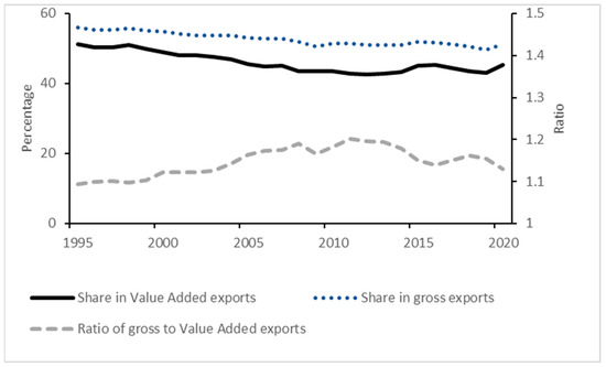
Figure 1.
Share of manufacturing in world gross and Value Added content of exports, 1995–2020. Source of data: TiVA 2023 indicators accessed on 2 April 2024. Calculations by the authors. Note: Calculations based on current prices. World Value Added content of gross exports is total domestic Value Added content of countries.
Constant Value Added Share analysis employs the same formal structure as constant market share analysis, but the use of value added trade data requires the re-interpretation of the decomposition results. Traditional CMS analysis assesses a country’s exports relative to the world or a reference group of countries by decomposing a country’s export growth into market share and structural effects. The market share effect is the difference between the export growth rate of the country and the world and quantifies the changes in a country’s share in individual export markets attributable to changes in price and non-price factors. Structural effects measure the contribution of the country’s product and geographical specialization to export growth, whether its exports are geared towards the more dynamic segments of world demand, and whether the geographical destinations of its exports are growing above the world average (Pandiella 2015).
Moreover, in Constant Value Added Share analysis, the term Value Added Share effect is defined as the difference between the growth rate of a country’s domestic Value Added trade and the world Value Added trade. The Value Added Share effect thus replaces the traditional market share effect which, in the CMS application, is a measure of competitiveness (Pandiella 2015). The Value Added Share effect also measures competitiveness, in this case in terms of the gain or loss of a country’s domestic Value Added (excluding the influence of differences in relative specialization) in comparison with world Value Added. Although outsourcing and offshoring may also influence competitiveness in value added, the Value Added Share effect can be considered a general indicator of a country’s performance in global value chains.1
Constant Value Added Share analysis also enables an alternative understanding of the decomposed structural effects. A key idea underlying the traditional CMS analysis applied to gross trade flows was the interplay of product structure and geographical export destination. Even if a country’s share of each product remains constant in all export destinations, a total decline in its market share is still possible if its export destinations are growing more slowly compared to the world average (Magee 1975). This intuition also applies very well to our approach to use Value Added data, with the interpretation that even if a country’s Value Added Share in all its exports remains the same in all its export destinations, a decline in total Value Added Share could still occur when its export destinations are not as dynamic as the world average. For example, even if a country consistently exports the same volume of high-technology products but the destinations of these products are growing slower than the world average, the country could still experience a loss in Value Added Share. Other concepts of CVAS analysis and the re-interpretation of the decomposition components will be discussed further in the section on methodology.
2. Literature Review and Contribution
Constant market share analysis (aka shift–share analysis) was first used in regional economics to track changes in productivity and employment. Tyszynski (1951) applied the methodology to trade economics in a study of manufactured commodities exports from 11 major countries in 1899–1950 and concluded that changes in relative trade position were due to a country’s ability to compete in specific commodity markets rather than structural shifts in world export demand. The core methodology was further developed as a decomposition process that analyses a country’s trade performance from the perspectives of competitiveness, export structure and specialization, and the geographical patterns and developments in major markets.
Leamer and Stern (1970) used export growth rates to decompose the total effect or export growth rate into structural and competitiveness effects. Initially, the results for the commodity and market effects varied slightly depending on the order in which these effects were calculated (Richardson 1971). Jepma (1981) introduced the “interaction effect” to avoid this arbitrariness and expanded the decomposition to five effects: scale, market, commodity, interaction, and static and dynamic. Milana (1988) proposed the interaction term “mixed effect”, which was adapted by Nyssens and Poullet (1990) into a two-stage decomposition: first, the competitiveness and structure effects, then the structure effect further decomposed into product, market, and mixed structure effects. The mixed structure effect is a residual that makes the computation insensitive to the order of decomposition. Note that the CMS formulation of Nyssens and Poullet (1990) as applied by Amador and Cabral (2008) and Pandiella (2015) is the basis for our Constant Value Added Share methodology.
Recent articles recommend improvements on the current formulation of the CMS methodology. Nuddin et al. (2018) propose a net-share decomposition approach to remove the interaction or residual term using a geometric framework. This new calculation intends to resolve the index number issue, which refers to how the decomposed effects are calculated in discrete time, in contrast to the continuously changing country and world export flows. Escaith (2020) proposes a new CMS formulation following the methodological features of revealed comparative advantage with the same objective of removing the residual. The resulting calculation may at first sight be a more straightforward statistical approach. However, there is an information loss in the removal of the residual and the second-level decomposition. While new approaches may contribute to a further refinement of the methodology, their viability stills need to be tested through empirical applications before gaining wide acceptance. Therefore, this article aims to contrast the novel Constant Value Added Share analysis with the standard CMS methodology rather than any new variant.
The empirical applications of the CMS method are abundant. Jepma (1981) applied CMS analysis to trade between the Associated African and Malagasy States and the European Community and concluded that negative export growth to the European Community was mainly due to the commodity effect and the market effect combined with a cyclical competitiveness. Oldersma and van Bergeijk (1993) investigated the trade patterns of the Netherlands, which then mostly comprised intra-European Union trade expressed in different currencies. Their study demonstrated how the choice of the currency in which the data are expressed in a fixed-exchange-rate regime influences the results of CMS analysis. Amador and Cabral (2008) tracked the evolution of Portuguese export performance over 40 years using a detailed product and geographical breakdown and a set of benchmark countries. The study concluded that the market share effect had the greatest impact on export performance.
Pandiella (2015) decomposed changes in Spain’s share in goods exports into competitiveness and structural effects and concluded that while Spain was more competitive than other European benchmark countries, a larger weight on relatively slow-growing goods destinations negatively impacted the country’s exports. Aguiar et al. (2017) investigated the evolution of market share of Bolivia, Brazil, and Peru in the Brazil nut sector and concluded that the loss of Brazilian market share was due to European market barriers and declining market growth. In contrast, Bolivia and Peru benefitted from an increase in exports to countries with higher growth rates. Gilbert and Muchová (2018) decomposed the export performance of eight Central and Eastern European economies using merchandise trade data and found that the gains in export competitiveness were tempered by a poor match to product and geographical partner profiles.
More recent studies apply the CMS methodology to the total or sectoral trade performance of developing countries. A study on the competitiveness of Pakistani leather goods (Maqbool et al. 2019) reported positive structural effects, but a negative competitiveness effect indicated a lack of product diversity. An assessment of the trade performance and export potential of Pakistan in the Central Asian republics (Kamal et al. 2021) showed that Pakistan is competitive in its top exports to the region. Research on China’s export performance by Bagaria and Ismail (2019) indicated a decreasing trend in competitiveness and a negative product structure effect, meaning that China is focused on products growing slower than the world average. Majdalawi et al. (2020) evaluated the date exports of Jordan and found fluctuations in the main decomposition effects attributable to annual changes in production and the import policies of market destinations. Fu et al. (2021) analyzed fruit exports from Hainan, China and showed that higher labor costs decreased price competitiveness.
Achentalika and Msuya (2022) applied the CMS methodology to East African Community exports and found that improved competitiveness and the composition of the exported commodities contributed to growth. Kumar (2022) evaluated the major agricultural commodity exports of India and concluded that greater competitiveness is needed to meet high world demand. The study of Kamal et al. (2022) on the trade performance of Pakistan and ASEAN countries with China showed that higher demand increased Pakistani exports despite negative competitiveness.
The cited studies all used gross trade data to examine a country’s exports in a specific industry or compare bilateral trade in goods. This article attempts to contribute to the literature as a novel attempt to measure trade performance in global value chains (rather than bilateral trade) using value added trade data (in place of gross trade data) through a re-interpretation of the decomposition effects of the CMS methodology as CVAS analysis. We find that CVAS analysis reflects a greater loss of competitiveness than CMS analysis, suggesting a decreased competitive advantage in the specific global-value-chain activities in which the reference country, the Philippines, participates. The second-level decomposition results on structure effects indicate participation in high-value, high-technology global value chains but a concentration in less dynamic products or inputs in these supply chains.
The rest of the article is organized into three main sections. Section 3, Methodology, introduces the CVAS decomposition methodology and the data. Section 4, Results, presents the main results. In Section 5, Discussion, we discuss the findings, draw implications, and indicate possible future research.
3. Methodology
Constant Value Added Share analysis applies the CMS decomposition methodology to value added data. The focus on value added also suggests a re-interpretation of the results as indicators of country participation in global value chains. The Total Value Added Effect (TVE) is first calculated as the difference between the growth in a reference country’s domestic Value Added content of gross exports (g) and the growth in world or reference group’s Value Added content of gross exports (g*). The destination of domestic Value Added content of gross exports refers to each ij destination country, measured as domestic Value Added content of gross exports of product i to destination country j.
TVE = g − g* = ∑i ∑j θij gij − ∑i ∑j θ*ij g*ij
Further, is the percentage change in the reference country’s Value Added content of gross exports of product i to destination j in period t, is the share of product i to destination j in total domestic Value Added content of its gross exports in period t − 1, and and are the equivalent notions for the Value Added content of gross exports of the world (excluding the reference country). The Total Value Added Effect is positive if the growth in domestic Value Added content of gross exports is higher than world Value Added, implying a gain in Value Added Share. The Total Value Added Effect is further decomposed into two terms: the Value Added Share Effect (VSE), which is considered an indicator for competitiveness, and the Combined Structure Effect (CSE), which refers to the degree of product and geographical specialization.
TVE = VSE + CSE = VSE + PSE + GSE + MIX
The Value Added Share Effect (VSE) is the difference between the growth rate of domestic and world Value Added content of gross exports in each period, excluding the influence of the difference in relative specialization, as changes in growth rates are weighted using the product share structure of the previous period. Given the product and geographical structure of gross domestic exports, the growth rates of domestic and world Value Added content of gross exports are compared for each product i to each destination country j. The Value Added Share Effect for a specific product i (destination country j) is the sum over j (i) of this effect. By abstracting from changes in product and geographical structures, the Value Added Share Effect attempts to reflect the changes in Value Added Share attributable to changes in (price and non-price) competitiveness. The Value Added Share Effect can be calculated either by product (by summing the individual ij effects over the j countries) or by destination country (by summing the individual ij effects over the i sectors) effects.
The Combined Structure Effect (CSE) indicates which part of the total change in Value Added Share results from the influence of the relative product/geographical specialization of the reference country. The second-level decomposition of the Combined Structure Effect yields three effects.
Decomposition of Combined Structure Effect
The Combined Structure Effect considers both the product and geographical specialization of the domestic Value Added content of gross exports and comprises three decomposed terms: the product structure effect (PSE), the geographical structure effect (GSE), and the mixed structure effect (MIX).
CSE = PSE + GSE + MIX
The Product Structure Effect (PSE) attributes the change in the Value Added Share to the product specialization of the domestic Value Added content of gross exports, i.e., whether the domestic Value Added content of gross exports includes the more dynamic product segments of world demand.
The Geographical Structure Effect (GSE) measures the contribution of each geographical destination of a country’s Value Added content of gross exports. A positive Geographical Structure Effect means the composition of Value Added content in gross exports is more concentrated in destinations that are growing faster than the world average.
The Mixed Structure Effect (MIX) is a residual term that incorporates the impacts of both the product and geographical structures of exports.
Here,
- (share of product i in domestic Value Added content of gross exports);
- (share of product i in world Value Added content of gross exports);
- (share of destination country j in domestic Value Added content of gross exports);
- (share of destination country j in world Value Added content of gross exports);
- (growth rate of world Value Added content of product i);
- (growth rate of world Value Added content of destination country j).
Table 1 summarizes the decomposition effects and their interpretation for the traditional CMS analysis of aggregated trade data related to gross exports and our CVAS analysis of Value Added data as an indicator of country participation in global value chains. A positive total effect in CMS analysis means that a country’s exports are growing faster than the world average. In CVAS analysis, a positive total Value Added effect means that the Value Added content of the country’s gross exports in the global value chains where it participates is growing faster than world Value Added. This indicates robust integration and participation in global value chains. In principle, it is possible that a country’s Value Added Share of gross exports is growing even when its share of exports remains the same. Competitiveness in CMS analysis, seen as a positive market share effect, signifies that the country is gaining market share for its gross exports compared to world market share. Competitiveness in CVAS analysis, measured as a positive Value Added Share effect, indicates that the country’s Value Added Share in the specific segments of the global value chains where it participates is higher compared to world Value Added. This signifies having a competitive advantage in the specific segments or activities in the global value chains where the country participates.

Table 1.
Interpretation of positive decomposition effects for Constant Market Share versus Constant Value Added Share analyses.
Structural effects trace the part of the change in competitiveness attributable to the country’s relative product or geographical specialization. Positive structural effects in CMS analysis imply that a country’s products or markets are more concentrated in faster-growing products or markets in comparison with the world. In CVAS analysis, positive structural effects indicate that a country’s inputs (products) to the global value chain segments where it participates or the destination countries of these inputs are concentrated in inputs or destination countries growing above the world average. A positive CVAS product structural effect means domestic Value Added is concentrated in inputs that are growing faster than world Value Added average, implying a relative specialization in dynamic sectors in the global value chain. Similarly, a positive geographical effect in CVAS analysis means the concentration of a country’s Value Added content is in destination countries growing above the world Value Added average. This signifies a strategic alignment with destination countries with faster growing Value Added, implying that a country’s Value Added is enhanced when the Value Added of the countries where its inputs are shipped, meaning the next segments or processes in the global value chain, is growing above world Value Added. In principle, it is possible that the products in which a country’s Value Added Share is growing are different from the products in which its export market share is growing. Similarly, destination countries where a country’s Value Added Share is growing could be different from the markets where export share is growing.
A limitation to the use of any decomposition analysis is the index number problem: the choice of the base year and weights assigned to destination countries and products can greatly influence the size and sometimes the sign of the results (Milana 1988). This article calculates CVAS results yearly such that the effects over time have multi-year effects (Amador and Cabral 2008). The use of simple averages (Pandiella 2015) summarizes the yearly results over 25 years in five subperiods—1996–2000, 2001–2005, 2006–2010 (the Great Recession and its immediate aftermath), 2011–2015, and 2016–2020—and serves as the basis for the comparison of results.
The greater availability of value added data derived from input–output tables facilitates the study of product and service flows in global value chains. In principle, two sources are available for this kind of analysis: the World Input–Output Database (WIOD) and the OECD Trade in Value Added (TiVA) database. The WIOD was launched in 2011, covering 40 countries and 35 industries for 1995-2011, and was intended to inform research efforts on global supply chains (Timmer et al. 2015). The WIOD 2016 release covers 43 countries, 28 members of the European Union (as of 1 July 2013) and 15 major economies, and 56 sectors for 2000–2014. The long-run WIOD 2021 version 1.1 (LR-WIOD) released in March 2022 extends the database backwards to a longer time period (1965–2000) for 25 countries, accounting for 85% of world GDP (Woltjer et al. 2021).
The TiVA indicators were first released in 2013 and intend to provide better insight into inter-country trade dynamics too complex to be reflected in conventional gross trade statistics. The latest TiVA 2023 edition measures trade in value added indicators for 76 economies and 45 industrial sectors for the years 1995–2020. While the WIOD 2016 release lists more sectors (56), it covers fewer countries (43) and a less recent time period (up to 2011). Hence, our choice was the TiVA database, which is the source of Value Added data for this article. In any case, the use of value added data for trade decomposition analysis would not have been possible to explore before the first editions of the WIOD in 2011 and TiVA in 2013. Two TiVA indicators useful to understand a country’s participation in global value chains are backward participation, defined as intermediate imports embodied in exports, and forward participation, which is the domestic value added in partners’ exports and final demand. However, both backward and forward participation are expressed in percentages and unsuitable for decomposition analysis. This article uses the TiVA indicator gross exports for the CMS analysis and the domestic Value Added content of gross exports for CVAS analysis. The subsector for energy-related products including coke and refined petroleum products is excluded from all decomposition analyses to avoid distortions related to the volatility of oil prices, similar to other CMS analysis (Amador and Cabral 2008).
Additional information on the technological intensity of the Value Added exports of the Philippines in Appendix A matches the ISIC Revision 3 categories for R&D or technological intensities with the TiVA product classifications (Appendix B). Categories of product specialization may be useful to understand the position of a developing country in a global value chain and provide context to the CVAS decomposition results.
4. Results
The results of the constant market share analysis for Philippine manufacturing sectors in Section 4.1 are followed by the Constant Value Added Share analysis in Section 4.2. Section 4.3 compares the main results from the CMS and CVAS analyses to illustrate to what extent the application of the decomposition method to value added data and their re-interpretation yield different results and new information. Lastly, Section 4.4 extends the CVAS analysis to Philippine goods and services.
4.1. Constant Market Share Analysis for Manufacturing Exports
Table 2 shows the main results of the constant market share analysis for Philippine gross manufacturing exports. Export growth was higher in the first half of the total period 1996–2007, roughly before the Great Recession, compared to 2008–2020 and slightly higher (1% on average) than world exports in four out of five subperiods. The average annual export growth for 25 years was almost 5%, below world growth of 5.1%. The market share effect shows a decline in export competitiveness for 11 of the 25 years under study especially in 1996–2005, reflecting a loss of market share compared to the world benchmark. Figure 2 shows that the market share effect or competitiveness contributed more to the total effect, both positively and negatively, than the combined structure effect. Overall, negative total and market share effects indicate lower export growth and loss of competitiveness in 1996–2020.
Table 2.
Results of the constant market share analysis for manufacturing sectors, 1996 to 2020.
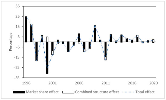
Figure 2.
Decomposition of the total effect, 1996–2020. Source of data: TiVA 2023 indicators accessed on 2 April 2024. Calculations by the authors.
In terms of structural effects, product structure contributed more to the combined structural effect than the geographical structure for most of the 25 years under study as seen in Figure 3. In 2001–2010, the product structure effect had a negative average, meaning that the country’s composition of exports was less concentrated in products growing above the world average. In contrast, the geographical structure overall had a slight but positive effect, which means that the composition of Philippine exports is more concentrated in export markets growing above the world average.
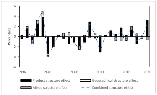
Figure 3.
Decomposition of the CMS combined structure effect, 1996–2020. Source of data: TiVA 2023 indicators accessed on 2 April 2024. Calculations by the authors.
4.2. Constant Value Added Share Analysis for Manufacturing Exports
Table 3 shows the two-level Constant Value Added Share decomposition analysis for Philippine manufacturing sectors for the same period (1996–2020). The total Value Added effect is the difference between the growth rates of country and world Value Added and is decomposed into the Value Added Share effect, a measure of competitiveness, and the combined structure effect, which indicates the relative product and geographical specialization. Overall, domestic Value Added did not outpace world Value Added, growing at par with an average less than 1%.
Table 3.
Results of the Constant Value Added Share analysis of gross manufacturing exports, 1996 to 2020.
In a year-by-year comparison, domestic Value Added grew less than world Value Added in 14 of the 25 years under study, significantly for half of the period after the Great Recession. The negative total Value Added effect corresponded to a negative Value Added Share effect, indicating a loss in competitiveness. The largest decrease in competitiveness was in 2001–2005, with the domestic Value Added Share at −7%. For the years 1996–2020, the Value Added Share effect averaged less than a percentage point. Figure 4 shows the greater contribution of the Value Added Share effect than the combined structural effect to the total Value Added effect for all years under study, except in 2020.
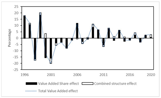
Figure 4.
Decomposition of the total Value Added effect, 1996–2020. Source of data: TiVA 2023 indicators accessed on 2 April 2024. Calculations by the authors.
Figure 5 shows the decomposition of the combined structure effect into product, geographical, and mixed structural effects. Product rather than geographical structure effect contributed more to the combined structure effect and was positive for around half of the years under study. This means that domestic Value Added was concentrated in products that were growing above the world average. Geographical structure effects for the years 1996–2020 were also mostly positive, meaning that the country destinations of the Value Added content of Philippine exports were, in general, growing above the world average. Both negative product and geographical structure effects contributed to a loss in competitiveness in the subperiod 2001–2005, but overall, the product and geographical effects were positive but contributed less than competitiveness to growth in the country’s Value Added. The mixed structure effect is a residual and includes the impact of both the product and geographical structures of exports.
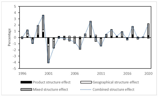
Figure 5.
Decomposition of the CVAS combined structured effect, 1996–2020. Source of data: TiVA 2023 indicators accessed on 2 April 2024. Calculations by the authors.
The manufacturing sectors where domestic Value Added is concentrated for the product structure effect are now discussed (Appendix C). The computer and electronics sector had the largest Value Added Share among product sectors in the overall period 1996–2020; however, this share was negative for all subperiods. Medium–high technology sectors, specifically machinery, transport equipment, and chemicals, contributed to offsetting this decline in the 25-year period at 1.1% compared to −1.0% for computer and electronics, with the total product effect averaging 0.1%. In addition, the computer and electronics sector is considered a high-technology sector (Appendix A and Appendix B). In principle, countries with a large share of high-technology goods face stronger world demand compared to lower-technology products (Pandiella 2015). In CVAS analysis, the negative product structure effects for the computer and electronics sector appear to indicate participation in high-technology global value chains but a concentration in less dynamic products or inputs in these supply chains.
Looking at the gain or loss in Value Added Share according to geographical destinations (Appendix D), the Philippines consistently gained a Value Added Share in Europe averaging 1.2% in 1996–2020. This means that domestic Value Added is concentrated in destination countries, specifically France and Germany, whose Value Added grew above the world average. This gain compensated for the loss of Value Added Share in North America and Asia. In 2001–2005, the negative geographical structure effect implies that domestic Value Added was concentrated in destination countries, specifically the United States and Japan, whose Value Added was growing less than world Value Added. The domestic Value Added Share was again less concentrated in destination countries with higher-than-world Value Added growth in the most recent subperiod, 2016–2020. Value Added in North America and Asia, specifically the United States, China, and Japan, which are the main destination countries for computer and electronics products, was growing less than the world average.
4.3. Comparison of CMS and CVAS Decomposition Results for Manufacturing Exports
The results of the constant market share and Constant Value Added Share analyses are compared using the arithmetic mean for 1996–2020 and five subperiods (Table 4). This comparison tests whether the application of the decomposition method to value added data and their re-interpretation yield different results and new information. In terms of the overall growth for the 25 years under study, CMS analysis shows a negative total effect, meaning that Philippine gross exports had lower growth compared to world exports. CVAS analysis shows that the country’s Value Added was only slightly higher than world Value Added of gross exports. A similar trend is observed for competitiveness in 1996–2020. There was a loss of market share compared to the world market share while there was a slight gain in the domestic Value Added Share compared to world Value Added Share of gross exports. Comparing within the subperiods, however (see Figure 6), CVAS results showed lower growth (a) and competitiveness (b) in 2001–2005 and 2016–2020. All CMS and CVAS results in 2001–2005 were negative; however, there was lower growth in Value Added compared to growth in exports, and the loss of competitiveness in Value Added was greater than the loss of competitiveness in export market share. In the most recent subperiod, 2016–2020, while CMS results register an upward trend from 2011–2015 for both growth in exports compared to world exports and a gain in market share compared to world market share, CVAS analysis shows much slower growth in Value Added and significantly lower competitiveness in Value Added compared to world Value Added. This divergence in results, especially in the most recent period, which is relevant for policy, and the greater number of years showing greater loss of competitiveness in Value Added than in market share, significantly after the Great Recession (as discussed in Section 4.1 and Section 4.2), show the usefulness of CVAS analysis and suggest the decreased competitive advantage in the specific global value chain activities where the Philippines participates.
Table 4.
Results for CMS and CVAS analysis for manufacturing, 1996 to 2020.
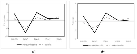
Figure 6.
Comparison of export growth (a) and competitiveness (b), measured via constant market share and Constant Value Added Share analyses, 1996–2020. Source of data: TiVA 2023 indicators accessed on 2 April 2024. Calculations by the authors. Note: Results are expressed in percentages. Averages show the mean (simple average).
The combined structure effects in both CMS and CVAS analyses appear to be less significant than competitiveness in accounting for the growth in exports and in the Value Added content of gross exports. Comparing the results in the subperiods (Figure 7), averages for CVAS product (a) and geographical (b) structure effects in 1996–2000 were lower than CMS structure effects. A similar trend is observed for the latest subperiod, 2016–2020, where lower averages for CVAS results indicate slower growth in the Value Added content of exports compared to gross exports and lower gain in Value Added competitiveness compared to gain in market share. Between the two structural effects, there is a bigger disparity in arithmetic means between CMS and CVAS product structural effects compared to geographical structure effects in the five subperiods. This may relate to the product specialization in gross exports being different from the Value Added contents of gross exports, which are assumed to be inputs in global value chains where the Philippines participates. In any case, the product structure appears to be an important factor to consider in the decomposition analysis and is examined more closely in the next section, where the scope of CVAS analysis is extended to Value Added in both products and services.
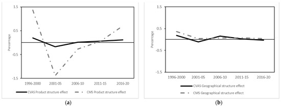
Figure 7.
Comparison of product (a) and geographical (b) structural effects measured via constant market share and Constant Value Added Share analyses, 1996–2020. Source of data: TiVA 2023 indicators accessed on 2 April 2024. Calculations by the authors. Note: Results are expressed in percentages. Averages show the mean (simple average).
4.4. Constant Value Added Share Analysis for Manufacturing and Services Exports
The Constant Value Added Share analysis is further applied to a wider dataset consisting of Philippine Value Added contents of export goods and services in the same period (Table 5). In general, the total Value Added results for the Philippines are better for the inclusion of both goods and services. The Value Added content of goods and services exports grew by 6.1% compared to 5.2% for the Value Added content of manufacturing exports (Table 4) in the years 1996–2020. Similar results for the total Value Added effect in the 25-year period, 1.2% for goods and services compared to 0.6%for manufacturing exports, indicate higher growth in domestic Value Added compared to world Value Added when export services are included. The Value Added Share effect was higher in three of the five subperiods (2001–2005, 2006–2010, and 2011–2015), and overall Value Added competitiveness in the total period 1996–2020 doubled, improving to 1% when both goods and services exports were used in the CVAS analysis.
Table 5.
Results of the Constant Value Added Share analysis of gross export products and services, 1996 to 2020.
Table 6 shows the gains and losses in Value Added Share competitiveness across the main product and service exports. Computer and electronic products in 2001–2005 (−3.0%) and 2016–2020 (−0.4%) contributed most to the decrease in overall competitiveness or the total Value Added Share effect in the subperiods (−1.8% and −0.4%). Expanding the decomposition analysis reveals the impact of industries other than manufacturing on Value Added performance. Low-technology product sectors, specifically food products and textiles, contributed significantly to the loss of Value Added competitiveness for the 25-year period. In contrast, service sectors, specifically information and communication services, offset the loss of Value Added competitiveness in computer and electronics products in 2001–2005 and even surpassed the sector’s competitiveness in 2006–2010. The overall competitiveness for information and communication services in 1996–2020 (0.3%) was higher than for all manufacturing sectors other than computer and electronics. These results support recent trade trends in the Philippines, which has seen sectoral growth in IT and business process management services that participate in IT-BPM global value chains (WTO 2021) and efforts to move up the computer and electronics sector to higher-value segments of the electronics and electrical parts and components global value chains (World Bank 2022).
Table 6.
Averages of Value Added Share effect for gross export products and services, 1996–2020.
5. Discussion
This article has analyzed a developing country’s participation in global value chains through the novel application of constant market share analysis as Constant Value Added Share analysis applied to value added trade data. The decomposition effects in CVAS analysis are re-interpreted as indicators of performance in global value chains. In the case of the Philippines, competitiveness in gross exports and Value Added exports was found to be the key factor in trade performance. CVAS reflects a greater loss of competitiveness than CMS analysis, suggesting a decreased competitive advantage in specific global value chain activities. These results are in line with the trade trends and policy direction related to the country’s participation in global value chains. The negative product structure effect derived through the CVAS analysis for the computer and electronics sector indicates a concentration in slower-growing Value Added products within the high-technology sector. This relates to current policy directions aimed to gear up the sector to enter higher-value segments in the computer and electronic parts global value chains. In addition, the increased Value Added competitiveness attributed to the information and communications services sector, measured through CVAS analysis for goods and services, relates to the country’s acknowledged participation and growth in IT-business process management global value chains.
The results of a decomposition analysis can be sensitive to the degree and level of decomposition. This article has addressed this caveat by first comparing the results of CMS and CVAS analysis on the country’s gross exports and Value Added content of manufacturing sectors and then widening the scope of CVAS analysis to goods and services. The variation yet complementarity in the results indicates that CVAS analysis measures something distinct from CMS analysis and that a growth in exports does not necessarily mean a growth in Value Added content. Further perspective into a country’s participation in global value chains was facilitated by linking CVAS analysis with the classification of the technological intensity of Value Added exports. While a country may have a significant percentage of Value Added in high-technology global value chains, the Value Added Share and product structure effects of CVAS analysis provide valuable insight on whether the country is contributing high or low Value Added exports within these high-technology production networks.
Evidence of the beneficial effects of global value chain participation is mixed (Ledda 2023), and CVAS analysis is a useful tool to assess developing-country participation and inform policy. It must be pointed out that CVAS analysis relies on value added trade indicators derived from inter-country input–output tables, which, in turn, are based on national supply and use tables. This means that CVAS analysis is available for developing countries and emerging markets with sufficiently robust statistical systems. Encouragingly, every update to the TiVA dataset includes more countries; the latest 2023 TiVA edition features 76 economies. For a robustness check on the results of CVS analysis, CMS analysis, which is also a decomposition analysis but based on more readily available gross trade data, can be performed.
Further refinements could be made to Constant Value Added Share analysis as a novel extension of the constant market share methodology. Countries in the same region could serve as the benchmark instead of the world for a reference country. This modification would facilitate insight into intra-regional trade, especially the movement of intermediate inputs in global value chains. Broadening the scope to inter-regional participation in global value chains can also be explored to focus on the interaction of the three manufacturing hubs of Europe, North America, and East Asia. Further understanding of the decomposition effects of CVAS analysis is also recommended. Some implications could be drawn between slow- and fast-growing destination countries and their positions or segments in the global value chain as expressed in the geographical structure effect. Nevertheless, as the article shows, Constant Value Added Share analysis has already demonstrated that it is an improvement over constant market share analysis and is a promising and recommendable tool to assess and gain insight into the participation of other developing countries in global value chains.
Author Contributions
G.M.L.: Conceptualization, Data Collection, Empirical analysis, Writing—original draft, Review & editing. P.A.G.v.B.: Conceptualization, Writing, Review & editing. All authors have read and agreed to the published version of the manuscript.
Funding
This research received no external funding.
Data Availability Statement
The original data presented in the study are openly available. See Gina M. Ledda (2024) Dataset by Gina M. Ledda, belonging to Constant Value Added Share Analysis: A Novel Trade Decomposition Technique. doi:10.25397/eur.26096893.
Acknowledgments
This article is part of a PhD project (Ledda 2023) and was presented at the 21st European Trade Study Group conference in Bern, Switzerland. Useful comments on earlier versions by participants, Charles van Marrewijk, and two anonymous reviewers are gratefully acknowledged.
Conflicts of Interest
The authors declare no conflicts of interest.
Appendix A. Technological Intensity of Value Added Exports
This appendix discusses Philippine and world product structures according to technological intensity using value added data. A comparison of Philippine and world Value Added content of gross manufacturing exports according to their technological content is offered as a support to the Value Added Share decomposition analysis. The four categories of manufacturing industries are based on research and development (R&D) or technological intensities (OECD 2011): high, medium–high, medium–low, and low technology content. The sectoral groupings in the TiVA database are more aggregated, however, and do not exactly match the OECD R&D intensity categories. Therefore, some adjustments had to be made. See Appendix B for the matched classifications.
Figure A1 compares the product structures of world Value Added and Philippine Value Added content according to technology intensity as proportions of total manufacturing sectors. Philippine Value Added content in high-technology products averaged 42% of total products across the 25-year period, more than double the world Value Added content average of 18%. In addition, the Philippines has its largest percentage of products in the high-technology classification (a). Countries that specialize or have a high share of high-technology goods are said to face stronger world demand for their products, in contrast to countries specializing in more low-technology products, which are seen as having less demand (Pandiella 2015). However, the Philippines had a higher proportion of Value Added content considered low-technology compared to world Value Added, with an average of 27% compared to 20%, indicating weaker demand for these products (d). The world share for medium–high technology products was higher than that of the Philippines: 41% compared to 17 (b). World Value Added was also greater than Philippine Value Added content in the medium–low technology classification of products, averaging 21% compared to 14% for the Philippines in 1995–2020 (c).

Figure A1.
Technological intensity of Value Added content of gross exports in 1995–2020 for high-technology (a), medium-high (b), medium-low (c), and low technology (d) products. Source of data: TiVA 2023 indicators accessed on 2 April 2024. Calculations by the authors. Note: Results are expressed in percentages. Averages show the mean (simple average).

Appendix B
Table A1.
Revision 3 Product Classification by Technological Intensity for Manufacturing Industries.
Table A1.
Revision 3 Product Classification by Technological Intensity for Manufacturing Industries.
| Industry | ISIC Rev. 3 | TiVA Product Classification |
|---|---|---|
| Manufacturing | 15–37 excl. 23 | D10T33 |
| High-technology industries | ||
| Aircraft and spacecraft | 353 | D29T30: Transport equipment |
| Pharmaceuticals | 2423 | D21: Pharmaceuticals, medicinal products |
| Office, accounting, and computing | 30 | D26: Computer, electronic, and optical products |
| Radio, TV, and communications equipment | 32 | D26: Computer, electronic, and optical products |
| Medical, precision, and optical instruments | 33 | D26: Computer, electronic, and optical products |
| Medium high-technology industries | ||
| Other electrical machinery, and apparatus | 31 | D27: Electrical equipment |
| Motor vehicles, trailers, and semi-trailers | 34 | D29T30: Transport equipment |
| Chemicals excluding pharmaceuticals | 24 excl. 2423 | D20: Chemicals and chemical products |
| Railroad and other transport equipment | 352 and 359 | D29T30: Transport equipment |
| Other machinery and equipment | 29 | D28: Machinery and equipment, nec |
| Medium low-technology industries | ||
| Building and repairing of ships and boats | 351 | D31T33: Other manufacturing; machinery repair |
| Rubber and plastic products | 25 | D22: Rubber and plastic products |
| Other non-metallic mineral products | 26 | D23: Other non-metallic mineral products |
| Basic metals, fabricated metal products | 27–28 | D24T25: Basic metals, fabricated metal |
| Low-technology industries | ||
| Other manufacturing and recycling | 36–37 | D31T33: Other manufacturing; machinery repair |
| Wood, pulp, paper, and printing products | 20–22 | D16T18: Wood and paper products; printing |
| Food products, beverages, and tobacco | 15–16 | D10T12: Food products, beverages and tobacco |
| Textiles, leather, and footwear | 17–19 | D13T15: Textiles, wearing apparel, leather |
Source of data: TiVA 2023 indicators accessed on 2 April 2024. Calculations by the authors. Note: Coke and refined petroleum products were excluded from CMS and CVAS analyses. Classification of TiVA product categories according to technological intensity was done by the authors.
Appendix C
Table A2.
Constant Value Added Share Analysis for Manufacturing Sectors, Product Structure Effect, 1996–2020.
Table A2.
Constant Value Added Share Analysis for Manufacturing Sectors, Product Structure Effect, 1996–2020.
| 1996–2000 | 2001–2005 | 2006–2010 | 2011–2015 | 2016–2020 | 1996–2020 | |
|---|---|---|---|---|---|---|
| High technology | −0.30 | −1.64 | −1.36 | −0.61 | −0.26 | −0.83 |
| Computer and electronic products | −0.36 | −1.90 | −1.62 | −0.71 | −0.30 | −0.98 |
| Pharmaceuticals | 0.06 | 0.27 | 0.26 | 0.11 | 0.04 | 0.15 |
| Medium–high technology | 0.67 | 1.97 | 1.74 | 0.64 | 0.27 | 1.06 |
| Electrical equipment | −0.04 | −0.15 | −0.07 | −0.03 | −0.02 | −0.06 |
| Machinery and equipment nec | 0.29 | 0.75 | 0.65 | 0.25 | 0.08 | 0.41 |
| Transport equipment | 0.23 | 0.92 | 0.76 | 0.21 | 0.17 | 0.46 |
| Chemical and chemical products | 0.19 | 0.46 | 0.41 | 0.20 | 0.04 | 0.26 |
| Medium–low technology | 0.07 | 0.21 | 0.32 | 0.28 | 0.12 | 0.20 |
| Rubber and plastic products | 0.03 | 0.11 | 0.09 | 0.04 | 0.02 | 0.06 |
| Other non-metallic mineral products | 0.01 | 0.01 | 0.00 | 0.01 | 0.00 | 0.01 |
| Basic metals and metal products | 0.08 | 0.08 | 0.14 | 0.20 | 0.07 | 0.11 |
| Manufacturing nec | −0.05 | 0.01 | 0.09 | 0.03 | 0.03 | 0.02 |
| Low technology | −0.24 | −0.72 | −0.69 | −0.25 | −0.02 | −0.38 |
| Food products, beverages, and tobacco | −0.05 | −0.61 | −0.75 | −0.27 | −0.07 | −0.35 |
| Textiles, wearing apparel and leather | −0.22 | −0.22 | −0.01 | 0.05 | 0.06 | −0.07 |
| Wood, paper products, and printing | 0.03 | 0.12 | 0.07 | −0.03 | −0.01 | 0.04 |
| Total | 0.20 | −0.17 | 0.02 | 0.06 | 0.12 | 0.05 |
Source of data: TiVA 2023 indicators accessed on 2 April 2024. Calculations by the authors. Note: Results are expressed in percentages. Averages show the mean (simple average). The total for each section is in bold.
Appendix D
Table A3.
Constant Value Added Share Analysis for Manufacturing Sectors, Geographical Structure Effect, 1996–2020.
Table A3.
Constant Value Added Share Analysis for Manufacturing Sectors, Geographical Structure Effect, 1996–2020.
| 1996–2000 | 2001–2005 | 2006–2010 | 2011–2015 | 2016–2020 | 1996–2020 | |
|---|---|---|---|---|---|---|
| Africa | −0.18 | −0.60 | −0.44 | −0.20 | −0.07 | −0.30 |
| Cameroon | 0.00 | 0.00 | 0.00 | 0.00 | 0.00 | 0.00 |
| Côte d’Ivoire | 0.00 | 0.00 | 0.00 | 0.00 | 0.00 | 0.00 |
| Nigeria | 0.00 | 0.00 | −0.01 | 0.00 | 0.00 | 0.00 |
| Senegal | −0.04 | −0.06 | −0.06 | −0.05 | −0.01 | −0.04 |
| South Africa | −0.14 | −0.55 | −0.37 | −0.16 | −0.06 | −0.25 |
| Asia | −0.14 | −0.98 | −1.15 | −0.45 | −0.15 | −0.58 |
| Bangladesh | 0.00 | 0.01 | 0.01 | 0.01 | 0.00 | 0.00 |
| Brunei Darussalam | 0.00 | 0.00 | 0.00 | 0.00 | 0.00 | 0.00 |
| Cambodia | 0.00 | 0.00 | 0.00 | 0.00 | 0.00 | 0.00 |
| China | 0.04 | −0.22 | −0.27 | −0.02 | −0.03 | −0.10 |
| Hong Kong (China) | 0.00 | 0.00 | −0.07 | −0.03 | −0.02 | −0.02 |
| India | 0.02 | 0.05 | 0.05 | 0.04 | 0.01 | 0.03 |
| Indonesia | 0.01 | −0.03 | −0.06 | −0.03 | 0.00 | −0.02 |
| Japan | −0.10 | −0.41 | −0.34 | −0.13 | −0.07 | −0.21 |
| Kazakhstan | 0.00 | 0.01 | 0.01 | 0.01 | 0.00 | 0.00 |
| Korea | 0.00 | −0.12 | −0.03 | 0.01 | 0.01 | −0.03 |
| Laos | 0.00 | 0.00 | 0.00 | 0.00 | 0.00 | 0.00 |
| Malaysia | −0.06 | −0.22 | −0.18 | −0.11 | 0.00 | −0.11 |
| Myanmar | 0.00 | 0.00 | 0.00 | 0.00 | 0.00 | 0.00 |
| Pakistan | 0.00 | 0.02 | 0.01 | 0.00 | 0.00 | 0.01 |
| Singapore | 0.02 | 0.06 | 0.06 | 0.03 | 0.01 | 0.04 |
| Chinese Taipei | 0.00 | −0.05 | −0.08 | −0.05 | −0.01 | −0.04 |
| Thailand | 0.03 | 0.09 | 0.09 | 0.05 | 0.02 | 0.05 |
| Viet Nam | −0.10 | −0.18 | −0.35 | −0.21 | −0.06 | −0.18 |
| Australasia | −0.01 | −0.03 | −0.01 | 0.01 | 0.00 | −0.01 |
| Australia | −0.01 | −0.04 | −0.02 | 0.00 | 0.00 | −0.01 |
| New Zealand | 0.00 | 0.01 | 0.01 | 0.01 | 0.00 | 0.01 |
| Central and South America | 0.05 | 0.14 | 0.15 | 0.06 | 0.02 | 0.08 |
| Argentina | 0.01 | 0.03 | 0.02 | 0.01 | 0.00 | 0.02 |
| Brazil | 0.03 | 0.08 | 0.08 | 0.03 | 0.02 | 0.05 |
| Chile | 0.00 | 0.01 | 0.02 | 0.00 | 0.00 | 0.01 |
| Colombia | 0.00 | 0.01 | 0.01 | 0.00 | 0.00 | 0.00 |
| Costa Rica | 0.00 | 0.00 | 0.00 | 0.00 | 0.00 | 0.00 |
| Peru | 0.00 | 0.01 | 0.01 | 0.01 | 0.00 | 0.01 |
| Europe | 0.79 | 2.32 | 2.00 | 0.69 | 0.23 | 1.21 |
| Austria | 0.03 | 0.07 | 0.07 | 0.02 | 0.01 | 0.04 |
| Belarus | 0.00 | 0.01 | 0.01 | 0.01 | 0.00 | 0.01 |
| Belgium | 0.04 | 0.08 | 0.07 | 0.03 | 0.00 | 0.04 |
| Bulgaria | 0.00 | 0.00 | 0.00 | 0.00 | 0.00 | 0.00 |
| Croatia | 0.00 | 0.00 | 0.00 | 0.00 | 0.00 | 0.00 |
| Cyprus | 0.00 | 0.00 | 0.00 | 0.00 | 0.00 | 0.00 |
| Czechia | 0.01 | 0.01 | 0.04 | 0.02 | 0.01 | 0.02 |
| Denmark | 0.02 | 0.04 | 0.03 | 0.01 | 0.01 | 0.02 |
| Estonia | 0.00 | 0.00 | 0.00 | 0.00 | 0.00 | 0.00 |
| Finland | 0.02 | 0.07 | 0.05 | 0.02 | 0.00 | 0.03 |
| France | 0.11 | 0.32 | 0.25 | 0.07 | 0.01 | 0.15 |
| Germany | 0.21 | 0.53 | 0.51 | 0.18 | 0.07 | 0.30 |
| Greece | 0.00 | 0.01 | 0.01 | 0.00 | 0.00 | 0.00 |
| Hungary | 0.00 | 0.00 | 0.01 | 0.00 | 0.00 | 0.00 |
| Iceland | 0.00 | 0.00 | 0.00 | 0.00 | 0.00 | 0.00 |
| Ireland | 0.02 | 0.07 | 0.06 | 0.02 | 0.01 | 0.04 |
| Italy | 0.12 | 0.37 | 0.28 | 0.09 | 0.04 | 0.18 |
| Latvia | 0.00 | 0.00 | 0.00 | 0.00 | 0.00 | 0.00 |
| Lithuania | 0.00 | 0.00 | 0.00 | 0.00 | 0.00 | 0.00 |
| Luxembourg | 0.00 | 0.01 | 0.01 | 0.00 | 0.00 | 0.00 |
| Malta | 0.00 | 0.00 | 0.00 | 0.00 | 0.00 | 0.00 |
| Netherlands | 0.02 | 0.03 | 0.03 | 0.00 | −0.01 | 0.02 |
| Norway | 0.01 | 0.01 | 0.02 | 0.01 | 0.00 | 0.01 |
| Poland | 0.01 | 0.05 | 0.06 | 0.03 | 0.01 | 0.03 |
| Portugal | 0.01 | 0.03 | 0.03 | 0.01 | 0.00 | 0.02 |
| Romania | −0.01 | −0.01 | −0.01 | −0.02 | −0.01 | −0.01 |
| Russia | 0.03 | 0.09 | 0.10 | 0.05 | 0.01 | 0.06 |
| Slovakia | 0.00 | 0.01 | 0.01 | 0.00 | 0.00 | 0.01 |
| Slovenia | 0.00 | 0.01 | 0.01 | 0.00 | 0.00 | 0.01 |
| Spain | 0.04 | 0.14 | 0.12 | 0.04 | 0.02 | 0.07 |
| Sweden | 0.05 | 0.13 | 0.10 | 0.04 | 0.01 | 0.07 |
| Switzerland | 0.04 | 0.11 | 0.10 | 0.05 | 0.02 | 0.06 |
| Türkiye | 0.01 | 0.06 | 0.05 | 0.02 | 0.01 | 0.03 |
| Ukraine | 0.00 | −0.03 | −0.08 | −0.04 | −0.01 | −0.03 |
| United Kingdom | −0.01 | 0.05 | 0.06 | 0.02 | 0.01 | 0.02 |
| Middle East and North Africa | 0.02 | 0.07 | 0.06 | 0.03 | 0.01 | 0.04 |
| Egypt | 0.00 | 0.01 | 0.01 | 0.00 | 0.00 | 0.00 |
| Israel | 0.01 | 0.03 | 0.02 | 0.01 | 0.00 | 0.01 |
| Jordan | 0.00 | 0.00 | 0.00 | 0.00 | 0.00 | 0.00 |
| Morocco | 0.00 | 0.01 | 0.01 | 0.00 | 0.00 | 0.01 |
| Saudi Arabia | 0.00 | 0.02 | 0.02 | 0.01 | 0.00 | 0.01 |
| Tunisia | 0.00 | 0.01 | 0.01 | 0.00 | 0.00 | 0.00 |
| North America | −0.40 | −1.23 | −0.65 | −0.19 | −0.11 | −0.52 |
| Canada | 0.04 | 0.13 | 0.07 | 0.01 | 0.00 | 0.05 |
| Mexico | 0.02 | 0.00 | −0.02 | −0.02 | −0.02 | −0.01 |
| United States | −0.46 | −1.36 | −0.70 | −0.19 | −0.10 | −0.56 |
| Rest of the World | 0.06 | 0.21 | 0.19 | 0.09 | 0.04 | 0.12 |
| Total | 0.19 | −0.10 | 0.15 | 0.03 | −0.03 | 0.05 |
Source of data: TiVA 2023 indicators accessed on 2 April 2024. Calculations by the authors. Note: Results are expressed in percentages. Averages show the mean (simple average). The total for each section is in bold.
Note
| 1 | The concept of competitiveness can be defined on several levels. In international trade, competitiveness is defined by the OECD as “a measure of a country’s advantage or disadvantage in selling its products in international markets” (OECD 2008). Firm-level competitiveness refers to a firm’s competitive advantage, defined as its ability to compete successfully in a specific business environment (Porter 1990). At the macroeconomic level, the World Economic Forum defines competitiveness as “the set of institutions, policies, and factors that determine the level of productivity of an economy” (Schwab 2016, p. 4). In this article, competitiveness can be understood in these traditional contexts. In addition, the use of value added trade data allows CVAS analysis to give insights into the competitiveness of a country in global value chains and the factors that affect this competitiveness and the overall country participation. |
References
- Achentalika, Harry Thomas Silas, and Dorah Teddy Msuya. 2022. Competitiveness of East African exports: A constant market share analysis. In Trade and Investment in East Africa. Edited by Binyam Afewerk and Peter A.G. van Bergeijk. Singapore: Springer, pp. 213–38. [Google Scholar]
- Aguiar, Giovanna Paiva, Joanna Duque Silva, José Roberto Frega, Lorena Figueira de Santana, and Jaqueline Valerius. 2017. The use of constant market share (CMS) model to assess Brazil nut market competitiveness. Journal of Agricultural Science 9: 174–80. [Google Scholar] [CrossRef][Green Version]
- Amador, João, and Sónia Cabral. 2008. The Portuguese export performance in perspective: A constant market share analysis. Banco de Portugal Economic Bulletin 14: 201–21. [Google Scholar]
- Bagaria, Nidhi, and Saba Ismail. 2019. Export performance of China: A constant market share analysis. Frontiers of Economics in China 14: 110–30. [Google Scholar]
- Bonanno, Graziella. 2014. A Note: Constant Market Share Analysis (Munich Personal RePEc Archive Paper No. 599997). Calabria: Department of Economics, Statistics, and Finance, University of Calabria. [Google Scholar]
- Escaith, Hubert. 2020. Contrasting Revealed Comparative Advantages When Trade Is (also) in Intermediate Products (MPRA Working Paper No. 103666). Marseille: Aix-Marseille University. [Google Scholar]
- Fu, Hailing, Chongli Huang, Zhuoqi Teng, and Yuantao Fang. 2021. Market structure, international competitiveness, and price formation of Hainan’s fruit exports. Discrete Dynamics in Nature and Society 2021: 6664780. [Google Scholar] [CrossRef]
- Gilbert, John, and Eva Muchová. 2018. Export competitiveness of Central and Eastern Europe since the enlargement of the EU. International Review of Economics and Finance 55: 78–85. [Google Scholar] [CrossRef]
- Jepma, Catrinus. 1981. An application of the constant market share technique on trade between the associated African and Malagasy States and the European community (1958–1978). Journal of Common Market Studies 20: 175–92. [Google Scholar] [CrossRef]
- Kamal, Muhammad Abdul, Saleem Khan, and Nadia Gohar. 2021. Pakistan’s export performance and trade potential in Central Asian region: Analysis based on constant market share (CMS) and stochastic frontier gravity model. Journal of Public Affairs 21: e2254. [Google Scholar] [CrossRef]
- Kamal, Muhammad Abdul, Unbreen Qayyum, Saleem Khan, and Bosede Ngozi Adeleye. 2022. Who is trading well with China? A gravity and constant market share analysis of exports of Pakistan and ASEAN in the Chinese market. Journal of Asian and African Studies 57: 1089–108. [Google Scholar] [CrossRef]
- Kumar, K. Nirmal Ravi. 2022. Competitiveness of Indian agricultural exports: A constant market share analysis. Research on World Agricultural Economy 3: 25–38. [Google Scholar] [CrossRef]
- Leamer, Edward E., and Robert M. Stern. 1970. Constant-market-share analysis of export growth. In Quantitative International Economics. Abingdon: Routledge, pp. 171–83. [Google Scholar]
- Ledda, Gina M. 2023. Heterogeneous Participation of Developing Countries in Global Value Chains. Ph.D. thesis, International Institute of Social Studies, Erasmus University Rotterdam, The Hague, The Netherlands. [Google Scholar]
- Ledda, Gina M. 2024. Dataset by Gina M. Ledda, belonging to Constant Value Added Share Analysis: A Novel Trade Decomposition Technique. [Google Scholar] [CrossRef]
- Magee, Stephen P. 1975. Prices, incomes and foreign trade. In International Trade and Finance: Frontiers of Research. Edited by Peter B. Kenen. Cambridge: Cambridge University Press, pp. 175–252. [Google Scholar]
- Majdalawi, Mohammad, Mohammad Al-Habbab, Amani Al-Assaf, Mohammad Tabeah, Salah-Eddin Araj, and Tawfiq M. Al-Antary. 2020. Improving supply chain of date palm by analyzing the competitiveness using a constant market share analysis. Fresenius Environmental Bulletin 29: 10997–1005. [Google Scholar]
- Maqbool, Muhammad Shahid, S. Anwar, and Mahmood T. Hafeez-Ur-Rehman. 2019. Competitiveness of the Pakistan in leather export before and after financial crises: A constant-market-share analysis. Journal of Global Economics 7: 1–7. [Google Scholar]
- Milana, Carlo. 1988. Constant-market-shares analysis and index number theory. European Journal of Political Economy 4: 453–78. [Google Scholar] [CrossRef]
- Nuddin, Aisha, A. Azhar, Vincent Gan, and Noor Khalifah. 2018. A new constant market share competitiveness index. Malaysian Journal of Mathematical Sciences 12: 1–23. [Google Scholar]
- Nyssens, A., and Ghislain Poullet. 1990. Parts de marche des producteurs deI’UEBL sur les marches exterieurs et interieur (Cahier 7). Brussels: Banque Nationale de Belgique. [Google Scholar]
- OECD. 2008. OECD Glossary of Statistical Terms. Paris: Organisation for Economic Cooperation and Development. Available online: https://read.oecd-ilibrary.org/economics/oecd-glossary-of-statistical-terms_9789264055087-en#page89 (accessed on 1 May 2022).
- OECD. 2011. ISIC REV. 3 Technology Intensity Definition: Classification of Manufacturing Industries into Categories Based on R&D Intensities. Paris: Organisation for Economic Cooperation and Development. [Google Scholar]
- Oldersma, Harry, and Peter A.G. van Bergeijk. 1993. Not so con$tant! The constant-market-share analysis and the exchange rate. De Economist 141: 380–401. [Google Scholar] [CrossRef]
- Pandiella, Alberto González. 2015. A Constant Market Share Analysis of Spanish Goods Exports (OECD Working Papers No. 1186). Paris: Organisation for Economic Cooperation and Development. [Google Scholar]
- Porter, Michael. 1990. The Competitive Advantage of Nations. New York: Free Press. [Google Scholar]
- Richardson, John David. 1971. Constant-market-share analysis of export growth. Journal of International Economics 1: 227–39. [Google Scholar] [CrossRef]
- Schwab, K. 2016. The Global Competitiveness Report 2016–2017. Geneva: World Economic Forum. [Google Scholar]
- Timmer, Marcel P., Erik Dietzenbacher, Bart Los, Robert Stehrer, and Gaaitzen J. de Vries. 2015. An illustrated user guide to the World Input–Output Database: The case of global automotive production. Review of International Economics 23: 575–605. [Google Scholar] [CrossRef]
- Tyszynski, Henry. 1951. World trade in manufactured commodities, 1899–1950. The Manchester School 19: 272–304. [Google Scholar] [CrossRef]
- Woltjer, Jop, Reitze Gouma, and Marcel P. Timmer. 2021. Long-Run World Input-Output Database: Version 1.0 Sources and Methods (GGDC Research Memorandum No. 190). Groningen: Rijksuniversiteit Groningen. [Google Scholar]
- World Bank. 2022. A New Dawn for Global Value Chain Participation in the Philippines. Edited by Guillermo Arenas and Souleymane Coulibaly. International Development in Focus Series. Washington, DC: World Bank. Available online: https://openknowledge.worldbank.org/server/api/core/bitstreams/73ea3565-605f-59ed-a982-c20b12b50524/content (accessed on 2 April 2022).
- WTO. 2021. Global Value Chain Development Report 2021: Beyond Production. Geneva: World Trade Organization. [Google Scholar]


Disclaimer/Publisher’s Note: The statements, opinions and data contained in all publications are solely those of the individual author(s) and contributor(s) and not of MDPI and/or the editor(s). MDPI and/or the editor(s) disclaim responsibility for any injury to people or property resulting from any ideas, methods, instructions or products referred to in the content. |
© 2024 by the authors. Licensee MDPI, Basel, Switzerland. This article is an open access article distributed under the terms and conditions of the Creative Commons Attribution (CC BY) license (https://creativecommons.org/licenses/by/4.0/).