Article

Quantifying Loss to the Economy Using Interrupted Time Series Models: An Application to the Wholesale and Retail Sales Industries in South Africa

by
Thabiso Ernest Masena
,
Sandile Charles Shongwe
* and
Ali Yeganeh
Department of Mathematical Statistics and Actuarial Science, Faculty of Natural and Agricultural Sciences, University of the Free State, Bloemfontein 9301, South Africa
*
Author to whom correspondence should be addressed.
Economies 2024, 12(9), 249; https://doi.org/10.3390/economies12090249
Submission received: 8 August 2024 / Revised: 31 August 2024 / Accepted: 14 September 2024 / Published: 17 September 2024

Abstract

:
A few recent publications on interrupted time series analysis only conduct preintervention modelling and use it to illustrate postintervention deviation without quantifying the amount lost during the intervention period. Thus, this study aims to illustrate how to estimate and quantify the actual amounts (in South African Rands—ZAR) that the negative impact of the intervention effects of the COVID-19 pandemic had on the South African total monthly wholesale and retail sales using the seasonal autoregressive integrated moving average (SARIMA) with exogenous components (SARIMAX) model. In addition, the SARIMAX model is supplemented with three approaches for interrupted time series fitting (also known as a pulse function covariate vector), which are: (i) trial and error, (ii) quotient of fitted values and actual values, and (iii) a constant value of 1 throughout the intervention period. Model selection and adequacy metrics indicate that fitting a pulse function with a trial-and-error approach produces estimates with the minimum errors on both datasets, so a more accurate loss in revenue in the economy can be approximated. Consequently, using the latter method, the pandemic had an immediate, severe negative impact on wholesale trade sales, lasting for 15 months (from March 2020 to May 2021) and resulted in a loss of ZAR 302,339 million in the economy. Moreover, the retail sales were also negatively affected, but for 8 months (from March 2020 to October 2020), with a 1-month lag or delay, suggesting the series felt the negative effects of the pandemic one month into the intervention period and resulted in a loss of ZAR 87,836 million in the economy.

1. Introduction

Intervention analysis provides a roadmap to modelling and estimating the intervention effect on a time series under study. In intervention analysis, the assumption is that the intervention affects the data-generating process by changing the mean function and trend of the underlying series (Cryer and Chan 2008). In general, interventions differ in magnitude and type. Some are natural (such as tsunamis and earthquakes), some are human-made (such as the 9/11 attack), and some have unknown causes, such as the COVID-19 pandemic (Bogoch et al. 2020; Wu et al. 2020). Since the onset of the COVID-19 pandemic, many researchers have conducted interrupted time series (ITS) studies to assess the impact of the pandemic throughout various fields. Most researchers used the naïve ordinary least squares segmented regression model to estimate and quantify the pandemic effects (McIntosh et al. 2021; Zhong et al. 2022; Yoshioka et al. 2022). Although segmented regression is a common approach, it is not always adequate, particularly when the data have seasonality and autocorrelation (Schaffer et al. 2021).
The Box–Jenkins autoregressive integrated moving average (ARIMA) models are an alternative approach to accommodate seasonality, autocorrelation and other potential confounding effects (Pridemore et al. 2014). Unlike in segmented regression, there is no need to include time and seasonal dummy variables in the ARIMA model, as the model can accommodate stochastic seasonality in the data. Stated differently, the first differencing is to remove a trend, and a seasonal difference is to remove the seasonality component so that the series can be transformed from nonstationarity to stationarity. The basic assumption of ARIMA modelling is that the data-generating process of the underlying time series does not change over time (Montgomery et al. 2015). However, in real-world applications, a time series may be subjected to interruptions, which affect the modelling and forecasting performance of the basic ARIMA models. As a result, Box and Tiao (1975) developed the autoregressive integrated moving average with exogenous components (ARIMAX) to incorporate these interventions into the series. The beneficial property of the ARIMAX model is that when conditions of the data-generating process of the underlying series are interrupted, the ARIMAX models are flexible and can be modified by using transfer functions to accommodate these changes (Inyang et al. 2023).
Transfer functions (or impact variables) provide a functional form of the characterised relationship between the intervention and the series under study. They reconstruct the relationship between the step, pulse, and time series to model more complex intervention impacts, including gradual level shifts, a pulse with gradual decay, and lagged effects (Box et al. 2015). The pulse and step functions are the two general types of transfer functions (Inyang et al. 2023). A step change is an abrupt, long-term change where the series level is moved either up or down by a particular value shortly after the intervention. A pulse is an abrupt, noticeable temporary change on one or more observations instantaneously after the intervention (Aliffia et al. 2024).
According to Bernal et al. (2017), it is important to hypothesise the probable shape of the resulting impact before conducting the intervention analysis. This can be done using the response variable’s pre-existing scientific knowledge and literature. Some intervention impacts are best represented by combining the step and pulse functions, and the resulting impact model can take different shapes and forms. A variety of impact models are found in (Montgomery et al. 2015; Bernal et al. 2017, 2018; and Bottomley et al. 2019). In ITS analysis, ARIMA produces forecasts of the underlying series in the absence of the intervention, referred to as the “counterfactual series”, which are used to evaluate how the actual values deviate from these forecasts in the intervention period (Bernal et al. 2017; Bartholomew et al. 2023). In the counterfactual scenario, the expected trend of the series remains unchanged. Therefore, the counterfactual series serves as a basis to compare the pattern of the interrupted series with how it would have unfolded had the intervention not occurred (Bartholomew et al. 2023).
In South Africa, the wholesale and retail sectors collectively contribute around 15% to the Gross Domestic Product (GDP), constituting approximately 22% of the country’s labour force (Sewell et al. 2016; Mamaro and Mabandla 2022). In particular, the retail sector is comprised of 87% small enterprises, 9.5% medium enterprises, and 4.5% large enterprises (Sewell et al. 2016). As a result of the strict COVID-19 measures, small retail enterprises were the most severely affected in the sector (Arndt et al. 2020). Large retail firms were no exception; for instance, the analysis of financial reports of twenty-two Johannesburg Stock Exchange (JSE)-listed South African retail firms showed that the COVID-19 pandemic had a statistically significant negative impact on the financial performance of these firms (Mamaro and Mabandla 2022). As shown in Chitiga-Mabugu et al. (2021), both the wholesale and retail sectors were among many other sectors of the South African economy that were severely affected by the COVID-19 pandemic. Thus, the COVID-19 pandemic had a negative impact (during the intervention period) on the employment level, job creation capability, and profitability of firms in these sectors, which had a direct detrimental effect on the overall South African economy. This highlights the importance of quantifying the approximate losses in the wholesale and retail sectors due to the COVID-19 pandemic. It is worth mentioning that there are other studies that explore tests of policy ineffectiveness when the predicted values of the variable of interest are computed using the reduced form or final form policy response equations (Pesaran and Smith 2016). Although the objectives of Pesaran and Smith (2016) and this study are aligned, which is to estimate the impact of the intervention or policy change on the target variable, the scope and objective of this study are different.
There is almost no research on the application of the ITS ARIMAX model in the context of the wholesale and retail sectors in South Africa and the rest of the world. However, similar research has been conducted in the past in other sectors to assess intervention effects with properties like COVID-19. For instance, in the health sciences, Zhou et al. (2023) used the ITS ARIMA approach to analyse the impact of the COVID-19 pandemic on the incidence rate of notifiable communicable diseases in China. ARIMA model with a change in slope that occurs immediately after the intervention was fitted to the data, and the results revealed a significant short-term decrease in the incidence rates of respiratory and enteric infectious diseases. Additionally, a short-term drop in the incidence rates of blood-borne and sexually transmitted infectious diseases with a step change was observed, which was likely to recover to the previous levels in the long term. There was no significant change in the incidence rate of natural focus diseases or arboviral diseases before and after the epidemic. In the oil industry, Aliffia et al. (2024) conducted a single-point intervention analysis with a pulse function to quantify the effect of the Russia–Ukraine conflict on the weekly price of crude oil. Among the models considered, ARIMA with a pulse function at the intervention point best fits the intervention series. The intervention parameters were estimated using the cross-correlation plot. The 12-week forecasts had relatively low model adequacy values (MAPE = 2.89% and MSE = 10.27). A study by Inyang et al. (2023) investigated the impact of the Declaration of Cooperation (DoC) by the Organisation of Petroleum Exporting Countries (OPEC) on monthly crude oil prices between January 1998 and December 2021. The Declaration of Cooperation had a statistically significant abrupt permanent increment of 33.72% to the price of crude oil immediately after it was introduced.
Lam et al. (2009) used an ARIMA model with a permanent step change to compute more precise and reliable estimates of the intervention effects and the asymptotic change observed in the business process reengineering simulation results from the activity model analysis. Bartholomew et al. (2023) investigated the effect of COVID-19 vaccinations on the daily COVID-19 cases in Nigeria using the naïve ordinary least squares linear regression model and the ITS ARIMA model. Five structural breaks were identified in the series, and the two models were fitted. Model selection metrics (AIC, BIC, and log-likelihood) showed that the naïve OLS regression model did not fit the data well and favoured the first differenced ITS ARIMA model with exogenous components. The intervention coefficient was negative, indicating that Nigeria’s daily cases remained high after the vaccine rollout.
In the legislature, Chamlin (2017) used ITS ARIMA with zero-order transfer functions to assess and model the impact of New Jersey’s blood and alcohol legislation on monthly total and separate mortalities of drivers and passengers from vehicle crashes. The results highlighted that the implementation of the blood and alcohol legislature had no significant effect on the number of deaths across all three outcome measures but proved to reduce vehicle crash fatalities by a rate of three passengers per month. In a similar study, Humphreys et al. (2013) studied the immediate and delayed impacts of removing regulatory trading hours restrictions on alcohol sales on the weekly police cases of violence in England and Wales. The analysis reported a gradual and permanent shift (step change) of violence between 3 a.m. and 6 a.m. by a first-order transfer function with an initial increase of 27.5% at the start of the intervention. It increased to 36% towards the end of the study period. Pridemore et al. (2014) assessed the effect of the implementation of the 2006 alcohol policy on gender-specific monthly alcohol-related fatalities of the Russian population aged 15 years and above. The intervention effect was modelled using a first-order gradual change ARIMAX intervention model. The study results showed that the introduction of the alcohol policy reduced the annual alcohol poisoning fatalities of approximately 6700 males as well as 760 male and 770 female liver cirrhosis fatalities. Had the policy not been introduced, male alcohol poisoning fatalities, female alcoholic liver cirrhosis, and male liver cirrhosis fatalities were estimated to have increased by 35%, 9%, and 15%, respectively.
In the South African context, studies using the Box–Jenkins methodology to independently investigate the long-term impact of the Global Financial Crisis (GFC) and COVID-19 pandemic on manufacturing, new car sales and the arrival of tourists were conducted (Makoni and Chikobvu 2023a, 2023b, 2023c; Chipumuro et al. 2024; Chikobvu and Makoni 2024). Similarly, Masena and Shongwe (2024a, 2024b) used the Box–Jenkins methodology with SARIMA with exogenous component (SARIMAX) to illustrate the effect of the COVID-19 pandemic on wholesale and retail sales in South Africa. Although these studies (Makoni and Chikobvu 2023a, 2023b, 2023c; Chipumuro et al. 2024; Chikobvu and Makoni 2024; Masena and Shongwe 2024a, 2024b) aimed to assess and quantify the intervention effect, there was no intervention analysis nor year-to-year comparisons evaluated to estimate the net loss in sales or revenue during the intervention period. Hence, this current study thoroughly extends on the work of Masena and Shongwe (2024a) and Masena and Shongwe (2024b) by conducting an in-depth intervention analysis by incorporating the pulse function into the fitted SARIMAX models in the intervention period; such an additional analysis assists in quantifying the approximate amount that the economy lost due the intervention period. This is the important component missing in all the publications (Makoni and Chikobvu 2023a, 2023b, 2023c; Chipumuro et al. 2024; Chikobvu and Makoni 2024; Masena and Shongwe 2024a, 2024b); readers must be made aware of these analyses so policymakers know the approximate amount lost due to an uncontrollable intervention. Then, mitigating strategies can be developed and implemented to lower the negative effects in the future. Furthermore, the intervention analysis uses three approaches to fitting the pulse function to the interrupted series throughout the intervention period for both the wholesale and retail series. Finally, the loss of revenue in both sectors will be quantified using the approach with the best-fitting pulse function.

2. Materials and Methods

In this study, T k represents the intervention period, where k = { 0 , 1 , , j } . T 0 is the starting point of the intervention and T j is the last point in the intervention period. Y t represents the response variables: the total monthly (i) wholesale and (ii) retail trade sales.
The step-change variable takes the value of 0 in the pre-intervention period and 1 during the intervention period (Cryer and Chan 2008). A step function is expressed as follows:
S t T k = 0 i f   t < T k 1 i f   t T k
The pulse variable takes the value of 1 in the intervention point/period and 0 otherwise (Cryer and Chan 2008). A pulse function is expressed as follows:
P t T k = 0 , if   t T k 1 , if   t = T k
For any given series, the intervention effect is modelled via the general form of a transfer function as follows (Schaffer et al. 2021):
Y t = μ + ω 0 + ω 1 B + ω 2 B 2 + + ω h B h 1 δ 1 B δ 2 B 2 δ r B r X t + ε t
where X t = P t T k or S t T k (intervention variable), B is the backshift operator ( B p Y t = Y t p ) ,   ω 0 denotes the initial value for the impact of the intervention at T 0 ,   δ is the decay rate, h describes when the effect happens, while r represents the decay pattern. When the intervention impact model shows that the intervention had an immediate effect with a gradual decay, h = 0 and r = 1 in Equation (3). However, when the intervention impact model shows that the intervention had a delayed effect with a gradual decay, h = 1 and r = 1 in (3). Note that r   =   1 is a variable used to show that the intervention impact in the series has an exponential decaying pattern or dies out exponentially.
Two parts of the overall model must be obtained to evaluate the impact of the intervention. The first part is the basic model for the pre-intervention series, and the second part is the intervention impact model (Bartholomew et al. 2023). The evaluation is carried out using the following steps:
  • Identify ( T 0 ) , the start of the intervention period;
  • Apply the Box–Jenkins methodology to fit an ARIMA model in the pre-intervention period;
  • Use the pre-intervention model to forecast values in the intervention period (counterfactual);
  • Obtain the differences between actual values in step (iii);
  • Evaluate step (iv) to determine a model for the intervention effect;
  • Use the results from step (v) to select the appropriate intervention variable;
  • Use Equation (3) to estimate the intervention effects.

3. Results and Discussion

This section outlines the ARIMA/SARIMA intervention models used to assess and quantify the COVID-19 pandemic effects on the total monthly wholesale and retail trade sales in South Africa. Section 3.1 summarises the pre-intervention models for the wholesale and retail datasets from the studies by Masena and Shongwe (2024a, 2024b). Section 3.2 presents the intervention analysis on the total South African monthly wholesale trade sales from April 2020 to May 2021 and the total South African monthly retail trade sales from April 2020 to October 2020. For both datasets, a pulse function is incorporated into the fitted SARIMA models using three approaches to extend the fitted pre-intervention models. All analyses involving model selection, parameter estimation, and model diagnostics were conducted using the TSA, tseries, forecast and MASS packages in R statistical software version 4.3.2 (Cryer and Chan 2008; R Core Team 2023; Trapletti and Hornik 2018; Hyndman and Khandakar 2008; Venables and Ripley 2002).

3.1. Pre-Intervention Models

3.1.1. Wholesale

The time series plot of the South African Wholesale trade sales from January 2009 until April 2023 is shown in Figure 1.
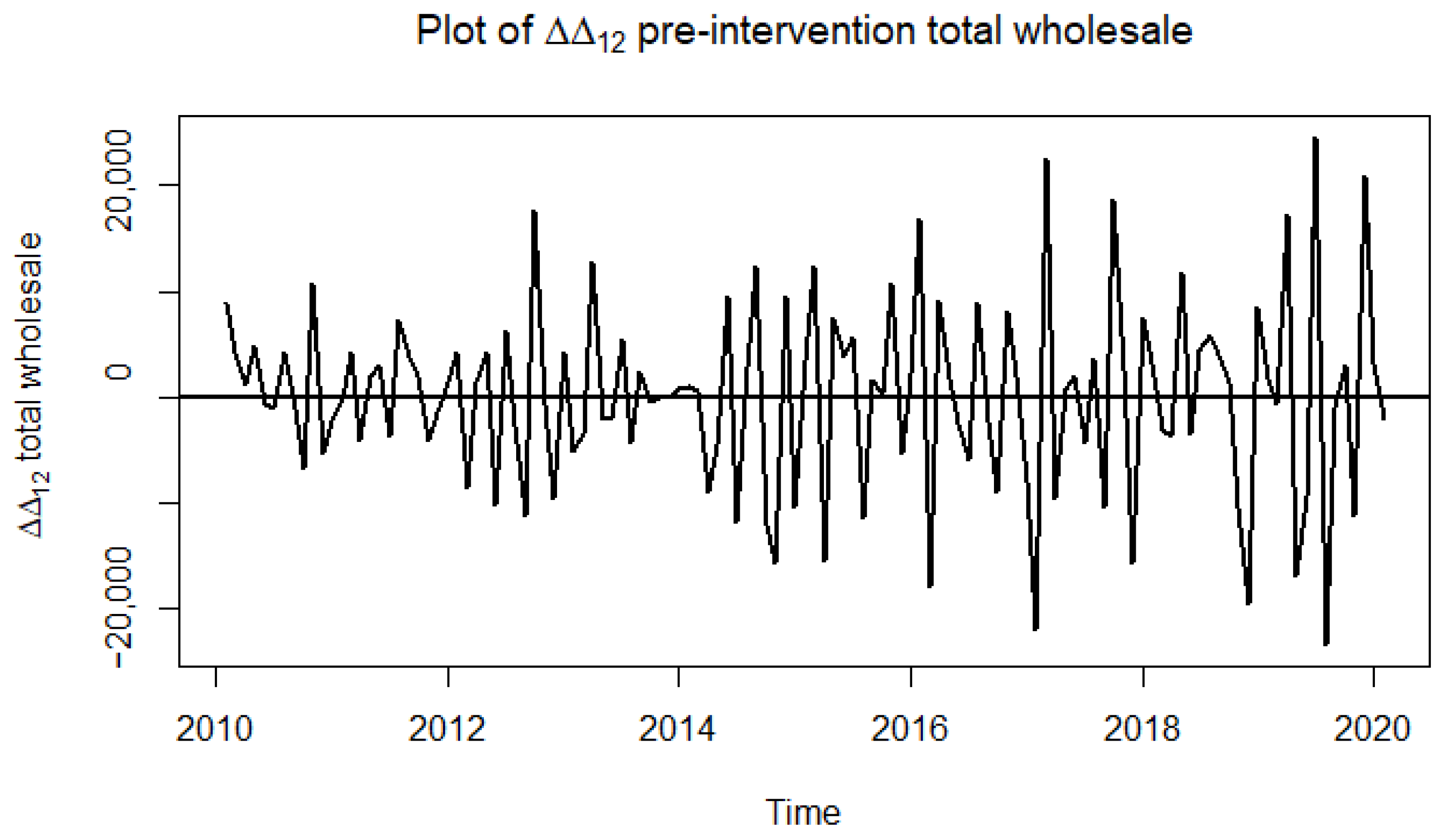
The Box–Cox transformation had a lambda value of λ = 1.0303 1 , which suggested that data transformation was not necessary for the wholesale data. The KPSS test has a highly significant p-value (0.01), which suggests that the series is not trend stationary. Therefore, the first and seasonal differences are necessary to de-trend and capture the seasonality in the series. The KPSS unit root test of stationarity was conducted, and its p-value 0.1; this means that it is not statistically significant at a 5% significance level. Therefore, the first and seasonally differenced wholesale series in Figure 2 is trend stationary.
Masena and Shongwe (2024a) identified the pre-intervention model for SA’s total monthly wholesale trade sales ( W t ) as SARIMA ( 2 , 1 , 1 ) 0 , 1 , 1 12 with MLE parameter estimates given in Table 1, and the model is given by:
1 ϕ 1 Β ϕ 2 Β 2 1 Β 1 Β 12 W t = 1 θ 1 Β 1 Θ 1 Β 12 ε t
All model parameters in Table 1 are statistically significant at the 5% significance level.
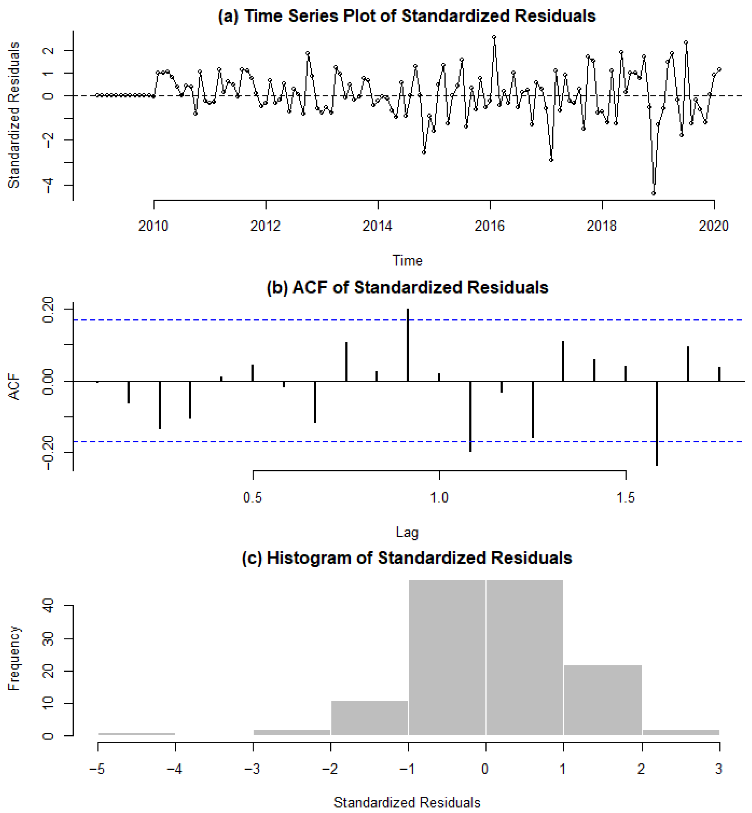
The standardised residuals in Figure 3a are random with no apparent trend. The ACF plot in Figure 3b suggests no autocorrelation on residuals except for 3 slightly significant lags. The pattern of the histogram of the residuals in Figure 3c is almost close to that of normal distribution. Shapiro–Wilk and Jarque–Bera normality tests were conducted at a 5% significance level. The highly significant p-values from the Shapiro–Wilk (0.01) and Jarque–Bera (4.006   ×   10 10 ) tests suggest that the standardised residuals from the fitted SARIMA model are not normally distributed. According to these tests, the assumption of normality is violated.
Portmanteau Ljung–Box and Box–Pierce tests are used to test for serial autocorrelation in the residuals of the chosen SARIMA 2 , 1 , 1 0 , 1 , 1 12 model. The p-values from the Ljung–Box (0.108) and Box–Pierce (0.149) tests are not statistically significant at a 5% significance level. Therefore, the null hypothesis cannot be rejected. It is concluded that there is no autocorrelation in the residuals from the fitted SARIMA model (since only a few lags exceed the standard error limits that are blue in Figure 3b). The slightly significant lags in Figure 3b are due to random sampling error.
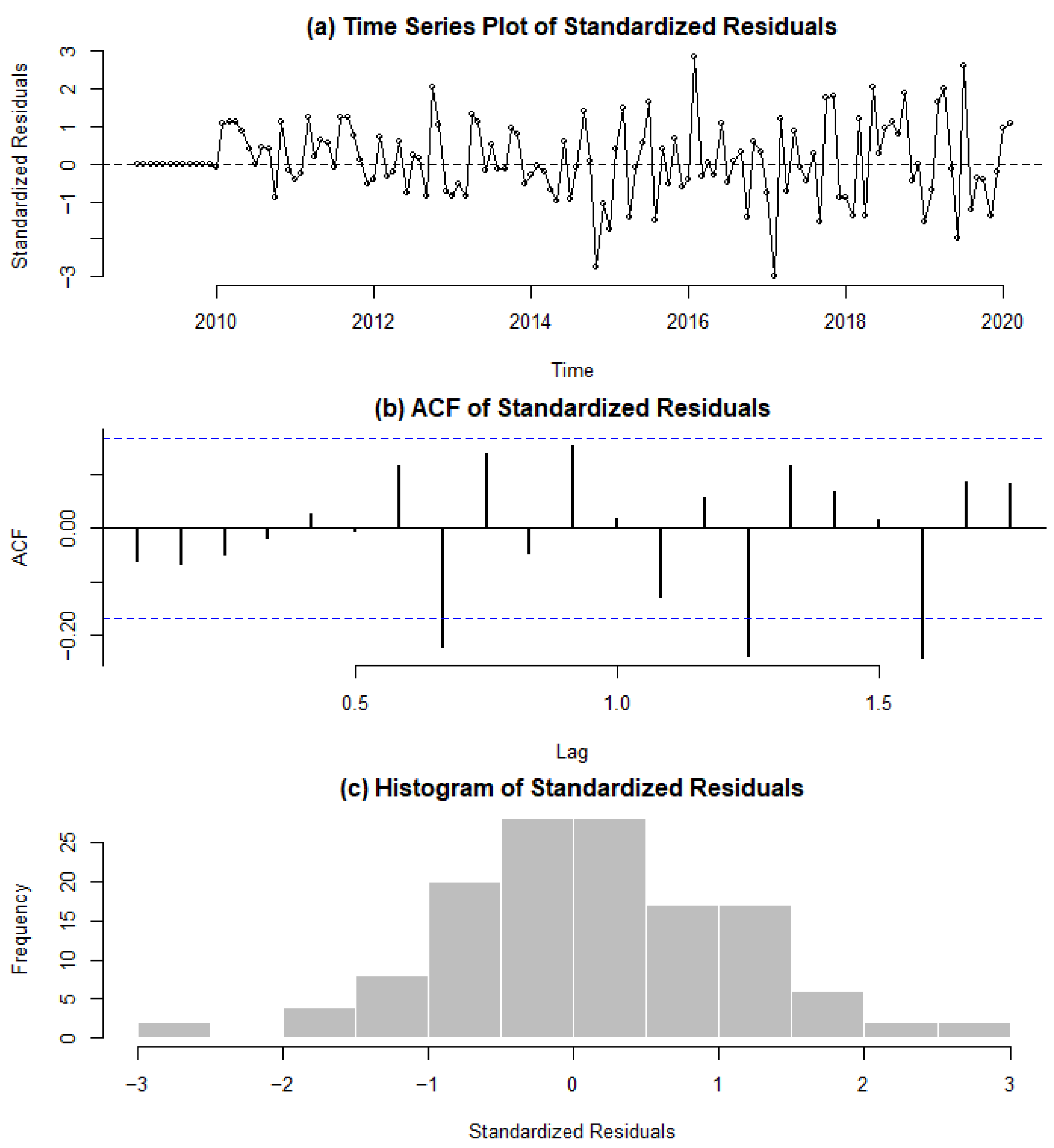
In further analysis, the fitted SARIMA 2 , 1 , 1 0 , 1 , 1 12 model was investigated for outliers in the pre-intervention period using the R forecast package (Hyndman and Khandakar 2008). An Innovative Outlier (IO) was detected at t 120 corresponding to December 2018. The presence of the IO explains the violation of the normality assumption. However, the histogram in Figure 4c suggests that the residuals from the SARIMA 2 , 1 , 1 0 , 1 , 1 12 model might be considered almost normally distributed. The p-value from the Ljung–Box (0.041) test is statistically significant at 5% significance level, suggesting autocorrelation in the residuals; this value is close to 0.05, indicating that the Ljung–Box test will have a non-significant p-value at 1% significance level. Moreover, the p-value from the Box–Pierce test (0.064) is not statistically significant at 5% significance level. Therefore, there is no notable autocorrelation in the residuals from the fitted SARIMA 2 , 1 , 1 0 , 1 , 1 12 model with the IO.

3.1.2. Retail

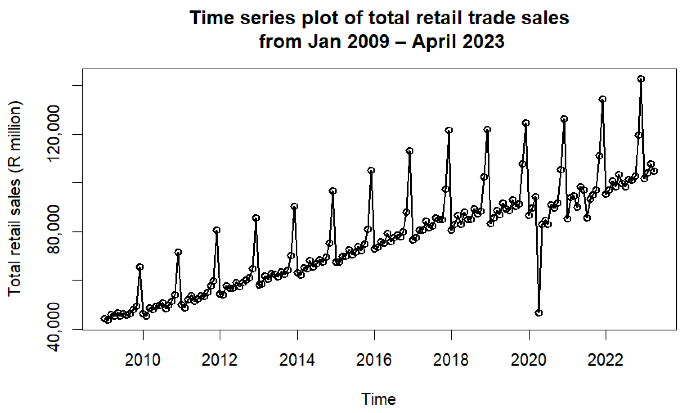
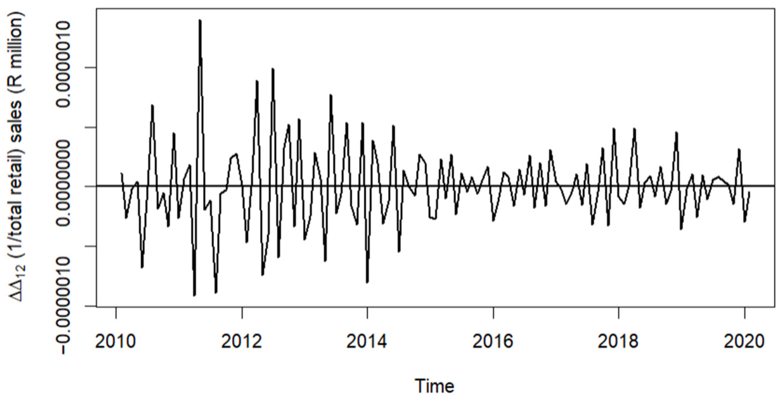
The time series plot of total monthly retail sales is given in Figure 5. The series in Figure 5 has an upward trend and exhibits a highly seasonal behaviour.
The first and seasonally differenced inverse transformed retail series in Figure 6 is stationary, with no apparent trend. The p-value (0.01) from the Augmented Dickey-Fuller (ADF) test is statistically significant at the 5% significance level. Therefore, the first and seasonally differenced inverse transformed retail series is stationary.
Masena and Shongwe (2024b) identified the pre-intervention model for SA’s total monthly retail trade sales ( R t ) as SARIMA ( 0 , 1 , 1 ) 0 , 1 , 0 12 with MLE parameter estimates given in Table 2. However, the mathematical expression for SARIMA ( 0 , 1 , 1 ) 0 , 1 , 0 12 in Masena and Shongwe (2024b) is incorrect. The correct mathematical expression of the SARIMA ( 0 , 1 , 1 ) 0 , 1 , 0 12 model is given by:
1 B 1 B 12 Y t = 1 θ 1 B ε t
where Y t = 1 R t , since the Box–Cox transformation suggested an inverse transformation to the retail data Masena and Shongwe (2024b). The model parameter in Table 2 is statistically significant at the 5% significance level.
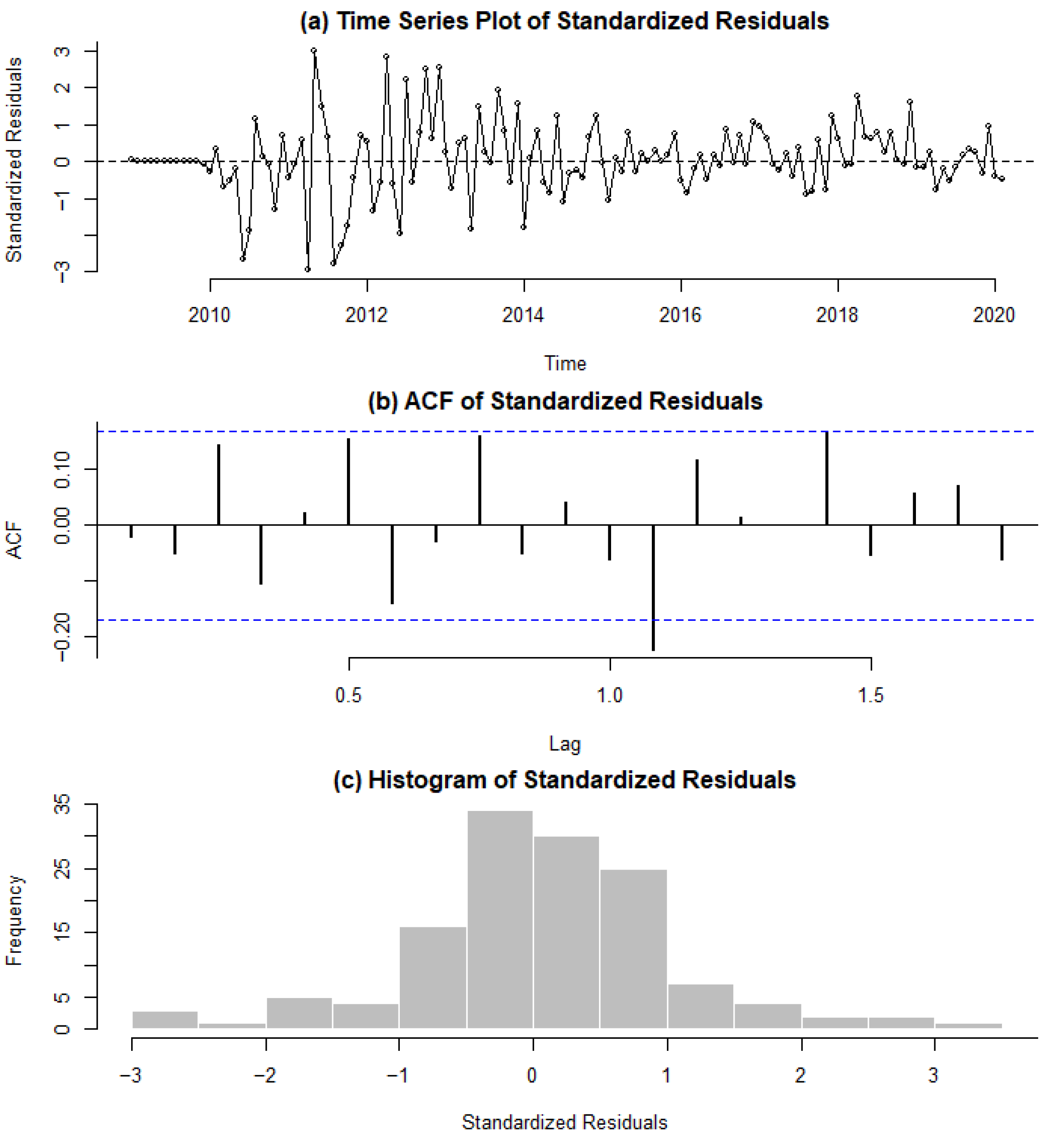
The time series plot, the ACF and histogram of standardised residuals from the fitted SARIMA 0 , 1 , 1 0 , 1 , 0 12 model is provided in Figure 7. The standardised residuals in Figure 7a are random with no apparent trend. The ACF plot in Figure 7b suggests no autocorrelation on residuals except for 1 significant lag. The pattern of the histogram of the residuals in Figure 7c almost resembles that of normal distribution.
The Portmanteau Ljung–Box and Box–Pierce tests are used to test for serial autocorrelation in the residuals of the chosen SARIMA 0 , 1 , 1 0 , 1 , 0 12 model. The p-values from both the Ljung–Box (0.208) and Box–Pierce (0.264) tests are not statistically significant at 5% significance level. Therefore, there is no autocorrelation in the residuals from the fitted SARIMA 0 , 1 , 1 0 , 1 , 0 12 model. Therefore, the SARIMA 0 , 1 , 1 0 , 1 , 0 12 model may be used to forecast future retail trade sales.

3.2. Intervention Analysis: Wholesale and Retail Sales

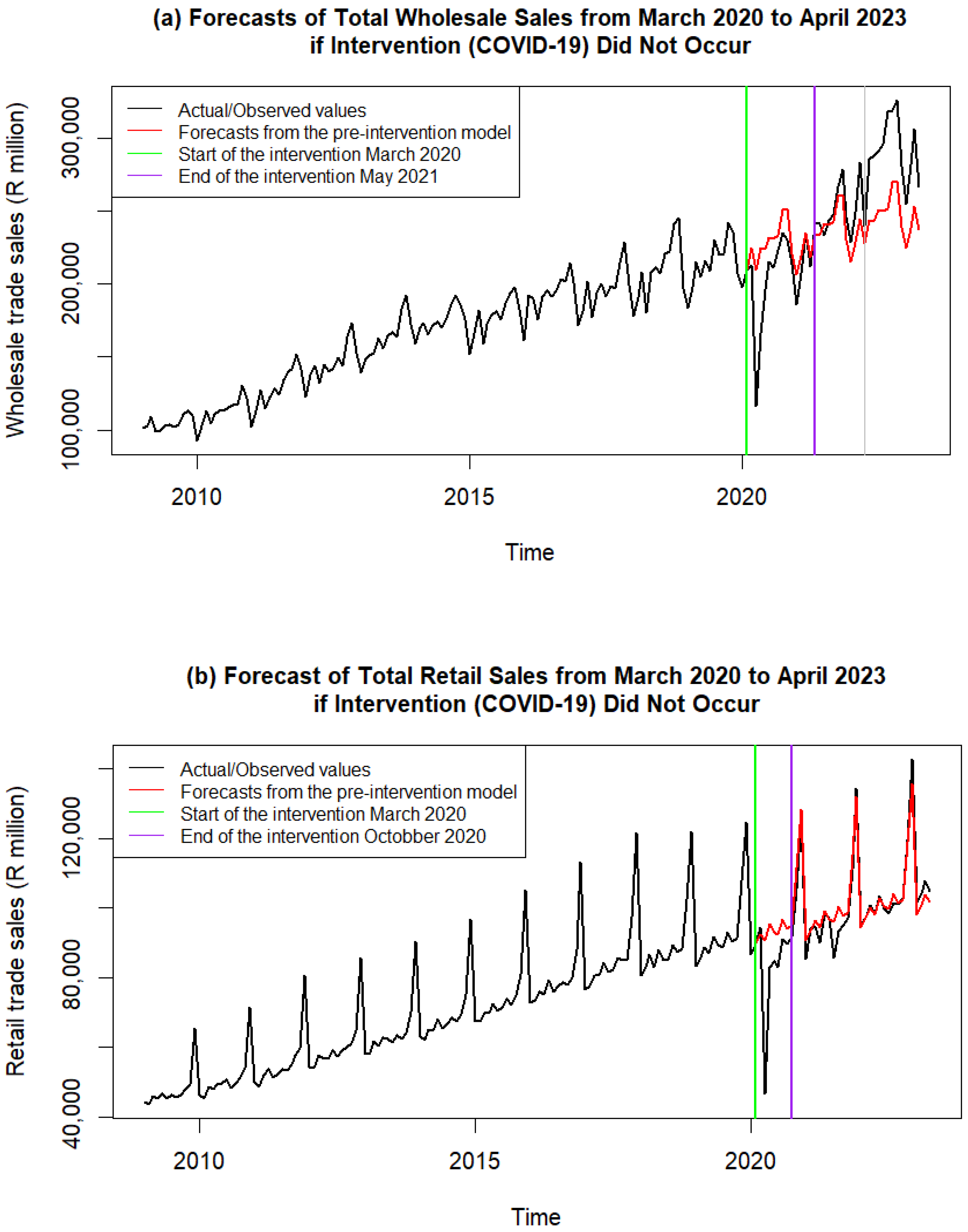
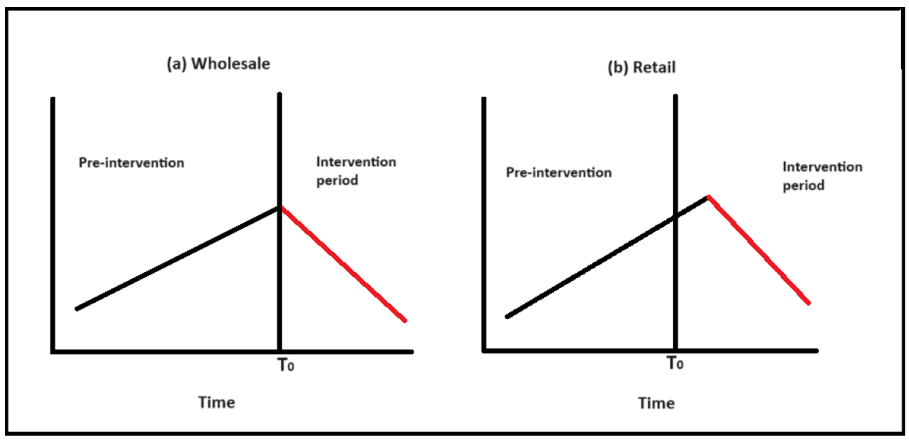
Figure 8 presents a broadened view of the pandemic impact on both the total monthly wholesale and retail trade sales from March 2020. In Figure 8a,b, forecasts generated using the pre-intervention model are used as the counterfactual series. That is, how the series would have evolved had the COVID-19 pandemic not occurred. Possible impact models of the COVID-19 intervention on wholesale and retail trade sales are illustrated in Figure 9. The graphical illustration in Figure 8a shows that it took 15 months (April 2020–May 2021) for the wholesale series to recover from the negative impacts of the pandemic. Therefore, it is concluded that the period from April 2020 to May 2021 is the intervention period in the context of the wholesale data. The Stats SA preliminary statistical release on the South African wholesale sector reported that April 2020 had the worst year-to-year (2019 to 2020) percentage change of −42.9% (Stats SA 2024a).
Moreover, there were positive year-to-year comparisons in September 2020 (1.2%) and December 2020 (2.9%). Most of the year-to-year comparisons in 2021 (2020 to 2021) are relatively better than those reported in 2020, with positive percentage changes in May 2021 (10.6%), April 2021 (82%) and May 2021(45.4%). More importantly, these year-to-year comparisons show that the pandemic had an immediate, negative impact on wholesale trade sales, as depicted in Figure 9a. On the contrary, the retail series took only 8 months to recover from the pandemic effects. Thus, the intervention period for the retail series is from March 2020 until October 2020.
From a different perspective, the Stats SA preliminary statistical release on the retail sector reported that April 2020 had the worst year-to-year (2019 to 2020) percentage change of −46.1% (Stats SA 2024b). There were positive year-to-year comparisons in March 2020 (6.4%), highlighting that the retail sales series felt the negative impact of the pandemic from the second month (1-month lag) in the intervention period, as illustrated in Figure 9b. September 2020 (1.2%) and December 2020 (2.9%) were reported to have shown positive year-to-year (2019 to 2020) percentage changes.

3.3. Three Approaches to Fitting a Pulse Function: Wholesale and Retail

3.3.1. Trial-and-Error Approach

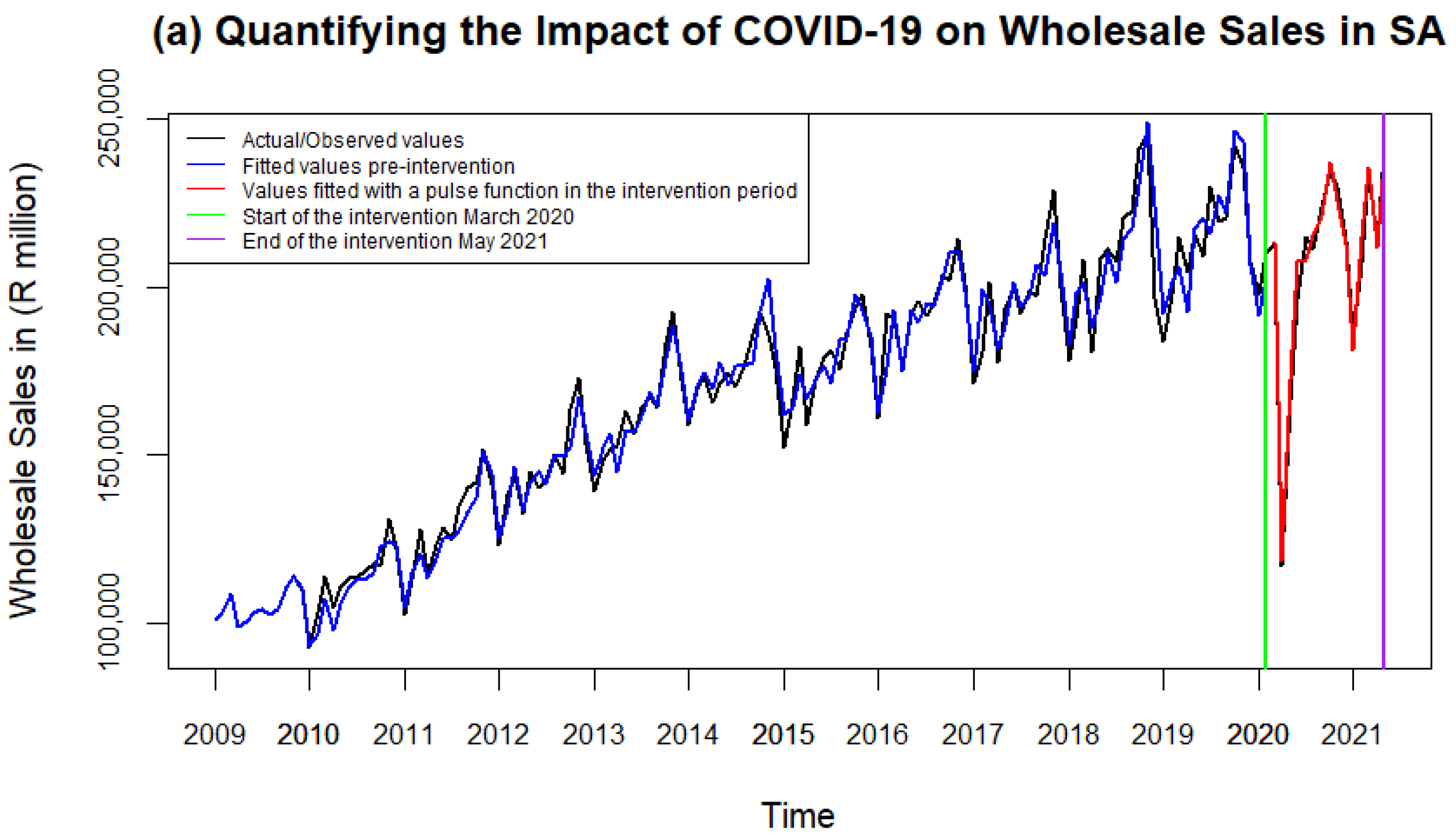
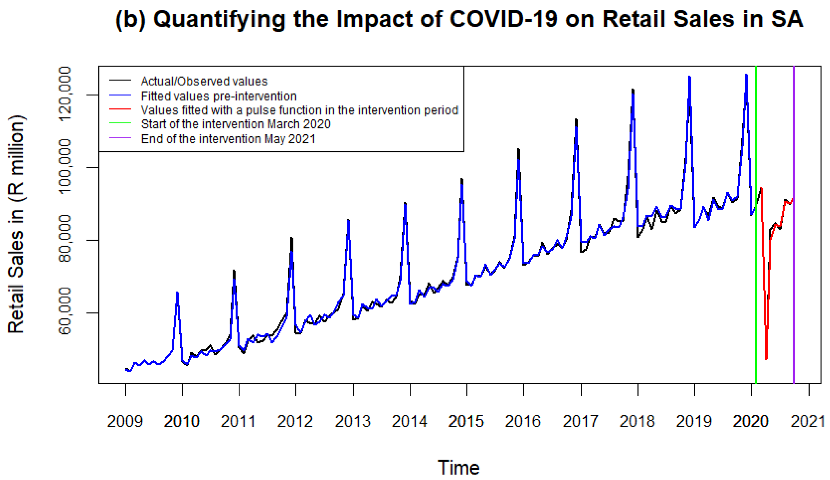
A pulse function is fitted on the counterfactual series to assess and model the effect of the pandemic on each observation. Figure 10 presents the results of the trial-and-error approach to fitting the pulse function.
The graphical analysis in Figure 10a shows that the fitted pulse function had a close to perfect fit to the wholesale series in the intervention period. The fitted values undeniably mimic the pattern of the actual/observed values in the same timeframe. The results are the same for the retail trade sales in Figure 10b. In this approach, the covariate vector of the fitted pulse function was determined through trial-and-error in R statistical software version 4.3.2, using the ‘xreg’ parameter in the arima function of the forecast package (Hyndman and Khandakar 2008).

3.3.2. Estimated Values/Actual Values (Quotient Approach)

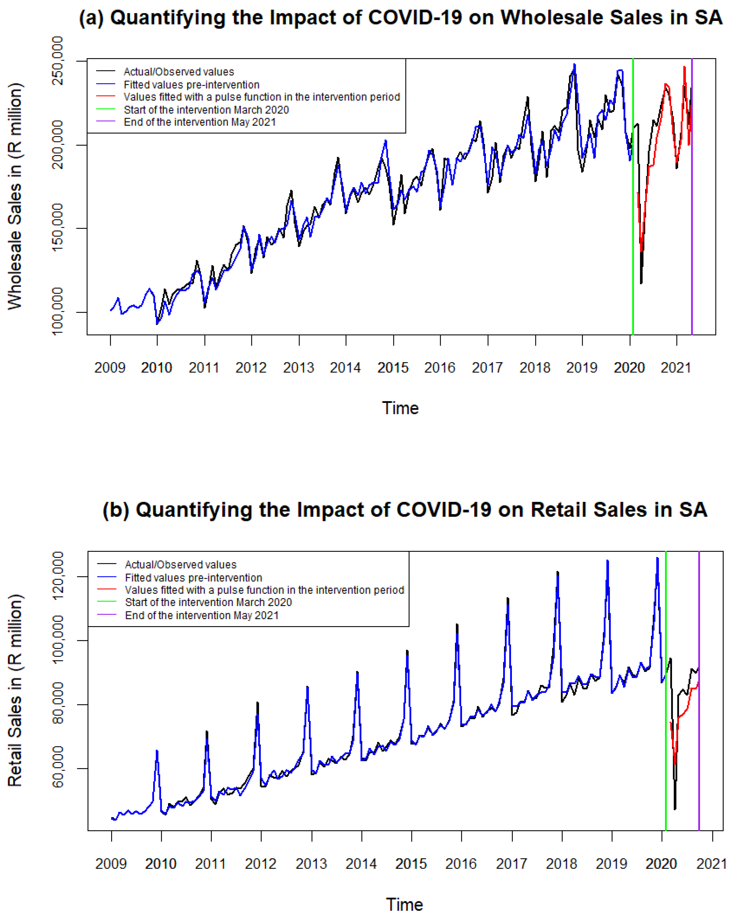
The second approach includes finding the covariate vector of the pulse function for each month by dividing the estimated or fitted value from the counterfactual series (forecasts) by the corresponding actual/observed value for that month throughout the intervention period. Figure 11 presents the results of the fit from this approach. Figure 11a,b show that fitting a pulse function in the counterfactual series using the quotient approach does not yield a better fit than the results shown in Figure 10 by the trial-and-error approach for both sectors. Although the series mimics the overall pattern of actual values in the intervention period, it could not capture the significant loss in sales recorded in April 2020 and a few subsequent points in the intervention period on both datasets.

3.3.3. P t = 1 , Where t = T k or 0 Otherwise

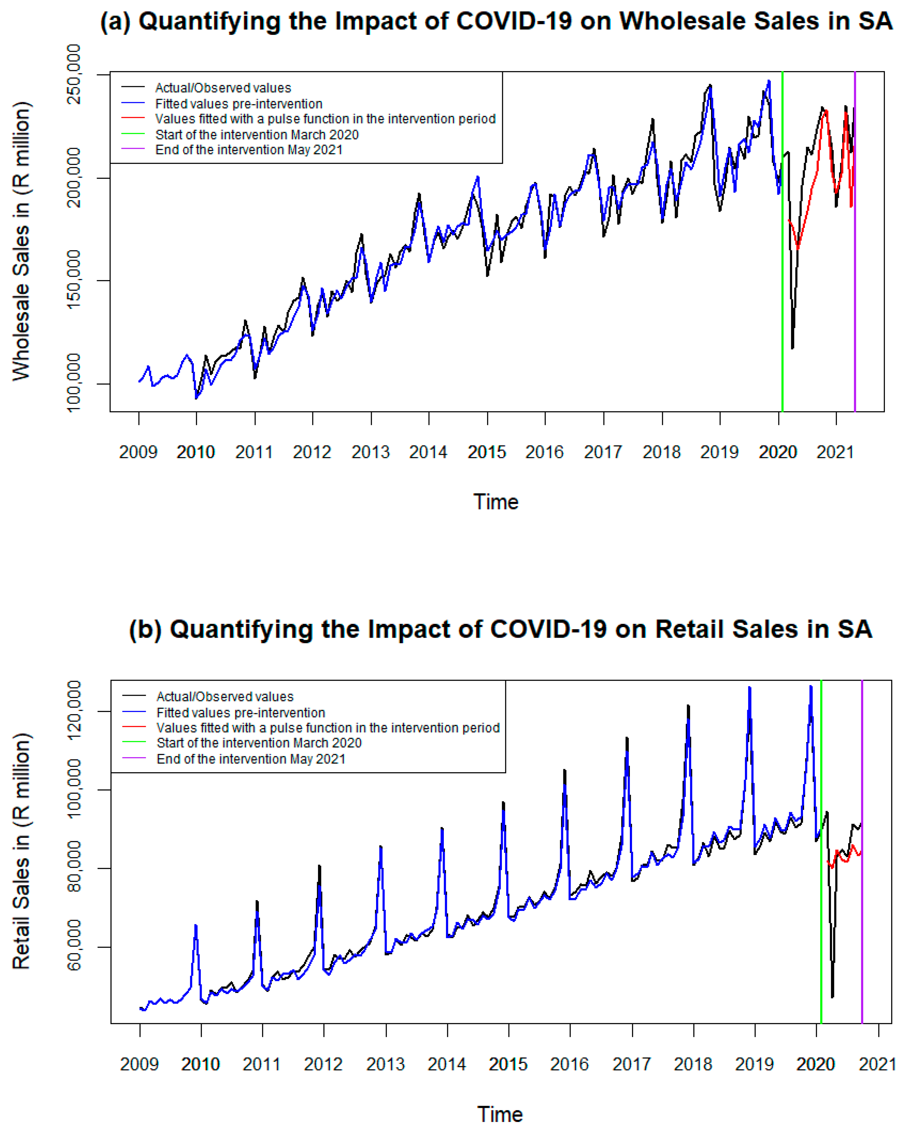
The third and final approach to fitting a pulse function is expressed in Equation (2), where the covariate vector in the pulse function is assigned a constant value of 1 throughout the intervention period and 0 in the pre-intervention period. This is the most common approach in interrupted time series intervention analysis (Pridemore et al. 2014; Inyang et al. 2023; Bartholomew et al. 2023). The results are shown in Figure 12. Although the fitted/estimated values from this approach managed to detect the negative impact of the pandemic on the actual trade sales, they do not capture its effect accurately. Figure 12a shows that fitting a pulse function using a constant value of 1 in the covariate vector does not provide a good fit to the wholesale series in the intervention period. The results are worse for the retail data shown in Figure 12b.

3.4. Approach Selection: Wholesale

Table 3 summarises the results of model selection and adequacy metrics from the three approaches used in fitting the pulse function on the interrupted wholesale series in the intervention period. From the results in Table 3, it is evident that Approach 1 is more appropriate in capturing the impact of the COVID-19 intervention on South African wholesale trade sales, as shown by the lowest Akaike’s information criterion (AIC), Bayesian information criterion (BIC), root mean squared error (RMSE) and the mean absolute percentage error (MAPE) values. Therefore, the model with the pulse function fitted by trial and error can be used to quantify the impact of the COVID-19 intervention on the total monthly wholesale trade sales.

3.5. Intervention Effects: Wholesale

Table 4 summarises the estimated intervention impact of the COVID-19 pandemic throughout the 15 months of the intervention period (highlighting the detrimental effect on wholesale trade sales). The percentage changes in Table 4 were calculated using Equation (6), expressed as:
%   C h a n g e = F i t t e d   v a l u e s T k P r e d i c t e d   v a l u e s T k P r e d i c t e d   v a l u e s T k × 100  
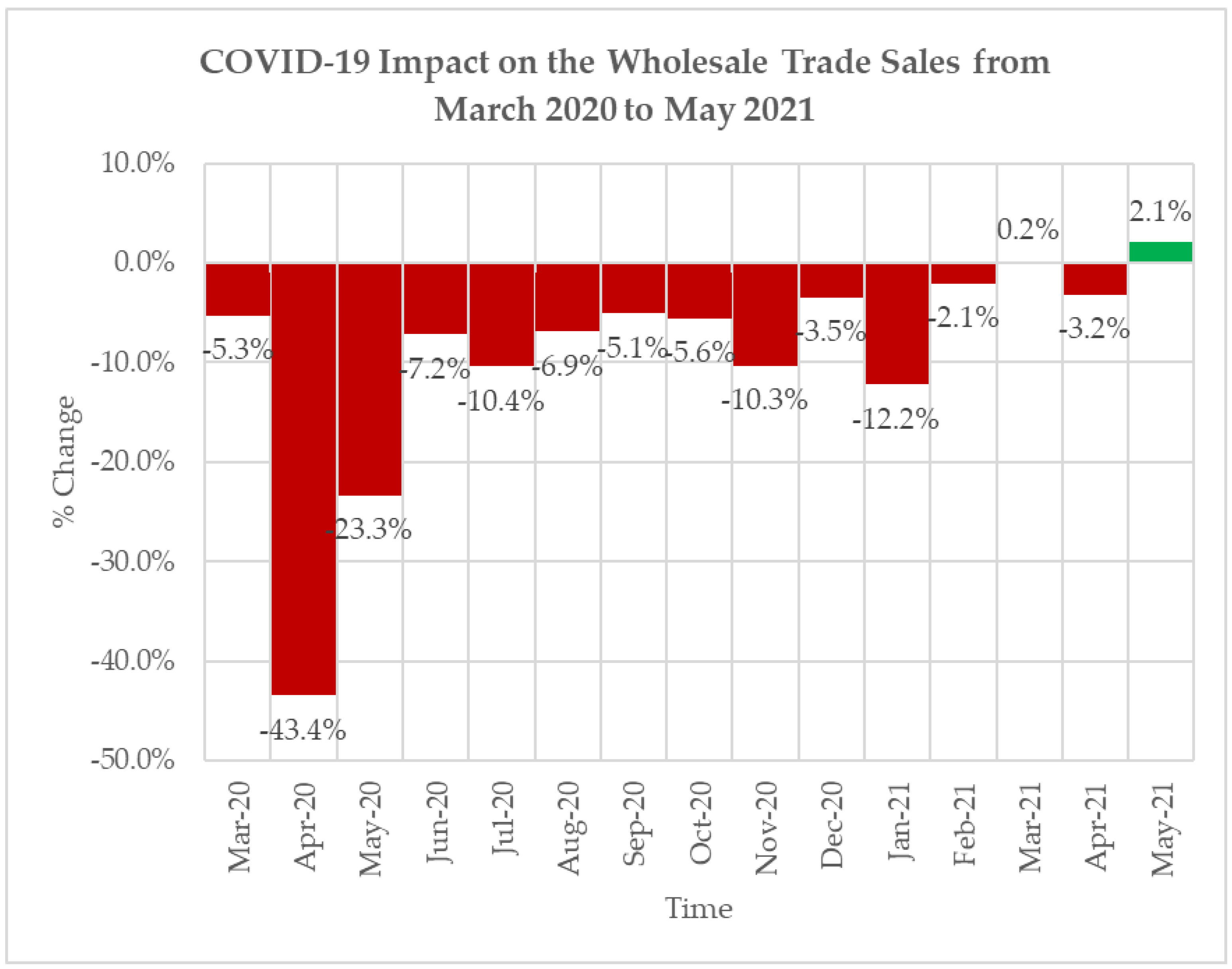
As shown in Figure 13, the hardest hit month was April 2020, with a 43.4% drop or ZAR 91,017 (million) fewer sales than it would have accumulated in the absence of the pandemic. May 2021 had a significantly high percentage change relative to all other months in the intervention period. This shows that not all months were negatively affected.

3.6. Approach Selection: Retail

Table 5 summarises the results of model selection and adequacy metrics from the three approaches used in fitting the pulse function on the perturbed retail series in the intervention period. Similar to the wholesale series, Approach 1 is more appropriate for capturing the impact of the COVID-19 intervention on South African retail trade sales, as shown by the lowest AIC, BIC, RMSE, and MAPE values. Therefore, the model with the pulse function fitted by trial and error can be used to quantify the impact of the COVID-19 intervention on the total monthly retail trade sales.

3.7. Intervention Effects: Retail

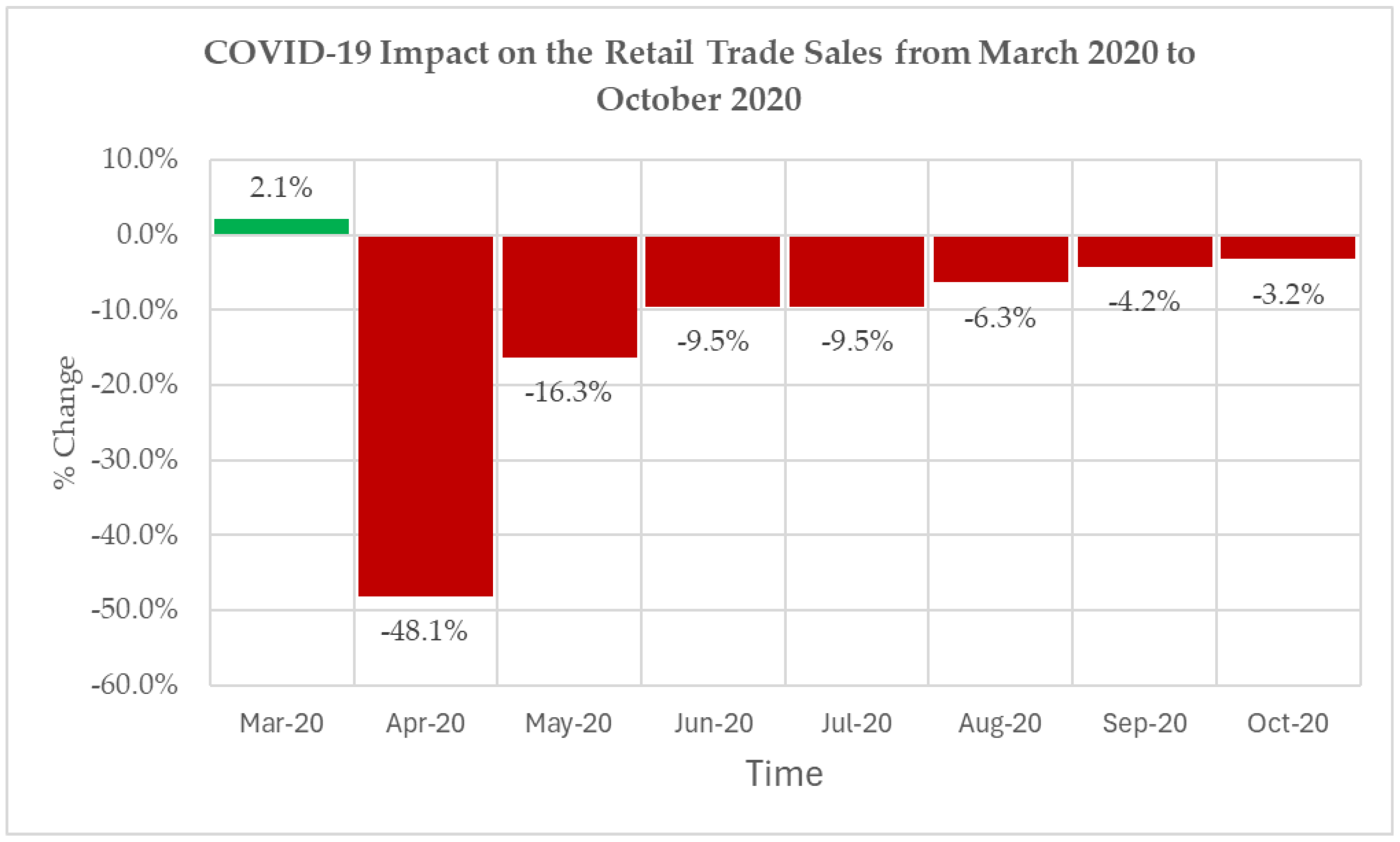
Table 6 summarises the estimated intervention impact of the pandemic on the retail trade series and is graphically illustrated in Figure 14. The percentage changes in Table 6 were calculated using Equation (6). The retail sector recorded a 48.1% drop or R43,534 (million) fewer retail sales than would have been accumulated in the absence of the pandemic in April 2020. This clearly indicates that April 2020 was the hardest-hit month in the intervention period. The plot of the estimated COVID-19 pandemic on the retail trade sales from March 2020 to October 2020, a total of 8 months, with a collective loss of ZAR 87,836 million.

4. Conclusions

This study aimed to estimate and quantify the intervention effects of the COVID-19 pandemic on the South African total monthly wholesale and retail sales using the ARIMA model with three approaches to fitting a pulse function covariate vector by: (i) trial-and-error, (ii) the quotient of fitted values and actual values (Quotient Approach) and (iii) a constant value of 1 throughout the intervention period. Model selection and adequacy metrics (AIC, BIC, RMSE, and MAPE) indicated that the trial-and-error method produced a covariate vector with the best-fitting pulse function in the intervention period for both datasets. Thus, the pulse function fitting using trial and error provides a new perspective on the ITS approach to intervention analysis. Interestingly, this approach has not been used in any studies or literature we consulted.
In this study, it is shown using the pulse function with the trial-and-error method that the pandemic had an immediate, severe negative impact on wholesale trade sales, lasting for 15 months (from March 2020 to May 2021). The retail sales were also negatively affected, but for 8 months only (March 2020 to October 2020), with a 1-month lag or delay, suggesting that the series felt the negative effects of the pandemic one month into the intervention period. The 8-month recovery period of the South African retail sector shows it is more resilient than the wholesale sector. In the analysis, it was shown that sales in both sectors were hardest hit in April 2020, with an estimated loss of ZAR 91,017 million and ZAR 43,534 million for the wholesale and retail trade sales, respectively. This is attributed to the implementation of the strict national lockdown, which came into effect on 27 March 2020 in South Africa. Furthermore, this is reflected by the extremely low year-to-year (2019–2020) comparisons and percentage changes between the counterfactual forecasts and the actual/observed values. In the intervention period, the total estimated losses in sales for the wholesale and retail sectors were ZAR 302,339 and ZAR 87,836 million, respectively, indicating that the wholesale industry had the worst losses.
The results of this study will strengthen the goal/objective to provide accurate and reliable forecasting techniques and approaches to quantifying the net effect of large-scale interventions on the two South African sectors. Given the importance of the wholesale and retail trade sectors in the South African economy (which accounts for a significant portion of the GDP and workforce), these intervention quantification efforts will aid businesses and policymakers in assessing the effectiveness of their countermeasures and allow them sufficient time to improve and allocate their resources efficiently to prepare for future shocks or interruptions. Using a time-series approach, one can analyse the trend of wholesale and retail trade sales before, during, and after the COVID-19 pandemic to identify the extent of the shock and forecast the industry’s future sales trajectory.
As part of future work, other researchers can reevaluate the work discussed in Makoni and Chikobvu (2023a, 2023b, 2023c), Chipumuro et al. (2024), and Chikobvu and Makoni (2024) to fit the pulse function model discussed here to conduct a proper quantification analysis of the intervention effect by estimating the actual loss in sales or revenue during the intervention (i.e., GFC or COVID-19) period in the South African economy. In addition, other alternative models may be more appropriate in the model selection process; some of these include hybrid models and machine learning methods. These can be pursued as future research and compared with the fitted model here.

5. Study Limitations

This study did not provide wholesale and retail trade sales forecasts in the post-intervention period using the selected ARIMAX intervention models. Moreover, the retail trade sales appear to have been subjected to a second intervention from June to July 2021; however, this plausible intervention was not investigated because the scope of this research was to assess the initial effect of COVID-19 on the two sectors in South Africa.

Author Contributions

Conceptualization, T.E.M., A.Y. and S.C.S.; methodology, T.E.M., A.Y. and S.C.S.; software, T.E.M. and S.C.S.; validation, A.Y. and S.C.S.; formal analysis, T.E.M.; investigation, T.E.M.; resources, S.C.S.; data curation, T.E.M.; writing—original draft preparation, T.E.M.; writing—review and editing, A.Y. and S.C.S.; visualization, T.E.M.; supervision, S.C.S. and A.Y.; project administration, S.C.S.; funding acquisition, S.C.S. All authors have read and agreed to the published version of the manuscript.

Funding

The research of the first author (T.E. Masena) is sponsored by Department of Science and Innovation (DSI) and the National Research Foundation (NRF) Masters Scholarship. The authors would like to acknowledge the Department of Mathematical Statistics and Actuarial Science and the Open Access Publication Fund at the University of the Free State for assistance with APC.

Institutional Review Board Statement

Not applicable.

Informed Consent Statement

Not applicable.

Data Availability Statement

This study uses the data indicated in Stats SA (2024a, 2024b).

Conflicts of Interest

The authors declare no conflicts of interest.

References

  1. Aliffia, Netha, Sediono Sediono, Suliyanto Suliyanto, Fariz Mardianto, and Dita Amelia. 2024. Modelling of world crude oil price based on pulse function intervention analysis approach. Media Statistika 16: 136–47. [Google Scholar] [CrossRef]
  2. Arndt, Channing, Rob Davies, Sherwin Gabriel, Laurence Harris, Konstantin Makrelov, Boipuso Modise, Sherman Robinson, Witness Simbanegavi, Dirk van Seventer, and Lillian Anderson. 2020. Impact of COVID-19 on the South African Economy-An Initial Analysis. SA-TIED Working Paper 111. Washington, DC: International Food Policy Research Institute. [Google Scholar]
  3. Bartholomew, Chekwube, Chrysogonus Nwaigwe, Ukamaka Orumie, and Godwin Nwafor. 2023. Intervention Analysis of COVID-19 Vaccination in Nigeria: The Naive Solution Versus Interrupted Time Series. Annals of Data Science 19: 1–26. [Google Scholar] [CrossRef]
  4. Bernal, Lopez, Stephen Soumerai, and Antonio Gasparrini. 2018. A methodological framework for model selection in interrupted time series studies. Journal of Clinical Epidemiology 103: 82–91. [Google Scholar] [CrossRef]
  5. Bernal, Lopez, Steven Cummins, and Antonio Gasparrini. 2017. Interrupted time series regression for the evaluation of public health interventions: A tutorial. International Journal of Epidemiology 46: 348–55. [Google Scholar] [CrossRef] [PubMed]
  6. Bogoch, Isaac, Alexander Watts, Andread Thomas-Bachli, Carmen Huber, Moritz Kraemer, and Kamran Khan. 2020. Pneumonia of Unknown Etiology in Wuhan, China: Potential for International Spread Via Commercial Air Travel. Journal of Travel Medicine 27: taaa008. [Google Scholar] [CrossRef]
  7. Bottomley, Christian, Anthony Scott, and Valerie Isham. 2019. Analysing Interrupted Time Series with a Control. Epidemiologic Methods 8: 1–10. [Google Scholar] [CrossRef]
  8. Box, George, and George Tiao. 1975. Intervention analysis with application to economic and environmental problems. Journal of the American Statistical Association 70: 70–79. [Google Scholar] [CrossRef]
  9. Box, George, Gwilym Jenkins, Gregory Reinsel, and Greta Ljung. 2015. Time Series Analysis: Forecasting and Control. Hoboken: John Wiley & Sons, pp. 428–77. [Google Scholar]
  10. Chamlin, Mitchell. 2017. An interrupted time series analysis of the differential impact of New Jersey’s BAC legislation on driver and passenger crash fatalities. Journal of Crime and Justice 40: 542–49. [Google Scholar] [CrossRef]
  11. Chikobvu, Delson, and Tendai Makoni. 2024. Modelling and Forecasting the Impact of the COVID-19 Pandemic on South Africa’s New Car Sales. Journal of Statistics Applications and Probability 13: 1127–40. [Google Scholar] [CrossRef]
  12. Chipumuro, Musara, Chikobvu Delson, and Makoni Tendai. 2024. Statistical Analysis of Overseas Tourist Arrivals to South Africa in Assessing the Impact of COVID-19 on Sustainable Development. Sustainability 16: 5756. [Google Scholar] [CrossRef]
  13. Chitiga-Mabugu, Margaret, Martin Henseler, Ramos Mabugu, and Hélène Maisonnave. 2021. Economic and distributional impact of COVID-19: Evidence from macro-micro modelling of the South African economy. South African Journal of Economics 89: 82–94. [Google Scholar] [CrossRef]
  14. Cryer, Jonathan, and Kung-Sik Chan. 2008. Time Series Analysis with Applications in R, 2nd ed. New York: Springer. [Google Scholar]
  15. Humphreys, David, Manuel Eisner, and Douglas Wiebe. 2013. Evaluating the Impact of Flexible Alcohol Trading Hours on Violence: An Interrupted Time Series Analysis. PLoS ONE 8: e55581. [Google Scholar] [CrossRef] [PubMed]
  16. Hyndman, Rob, and Yeasmin Khandakar. 2008. Automatic time series forecasting: The forecast package for R. Journal of Statistical Software 27: 1–22. [Google Scholar] [CrossRef]
  17. Inyang, Elisha, Edwin Nsien, Etebong Clement, and Dannjeh Agidi. 2023. Statistical Investigation of The Impact of Global Oil Politics: An Interrupted Time Series Approach. JP Journal of Mathematical Sciences 32: 1–13. [Google Scholar]
  18. Lam, Chiyung, Wai Ip, and Henry Lau. 2009. A business process activity model and performance measurement using a time series ARIMA intervention analysis. Expert Systems with Applications 36: 6986–94. [Google Scholar] [CrossRef]
  19. Makoni, Tendai, and Delson Chikobvu. 2023a. Assessing and Forecasting the Long-Term Impact of the Global Financial Crisis on Manufacturing Sales in South Africa. Economies 11: 158. [Google Scholar] [CrossRef]
  20. Makoni, Tendai, and Delson Chikobvu. 2023b. Evaluating and Predicting the Long-Term Impact of the COVID-19 Pandemic on Manufacturing Sales within South Africa. Sustainability 15: 9342. [Google Scholar] [CrossRef]
  21. Makoni, Tendai, and Delson Chikobvu. 2023c. Assessing and Forecasting the Long-Term Impact of the Global Financial Crisis on New Car Sales in South Africa. Data 8: 78. [Google Scholar] [CrossRef]
  22. Mamaro, Phulong, and Ndonwabile Mabandla. 2022. The influence of the COVID-19 pandemic on the financial performance of listed retail firms in South Africa. Acta Economica 20: 211–28. [Google Scholar] [CrossRef]
  23. Masena, Thabiso, and Sandile Shongwe. 2024a. Investigating the lingering effects of the pandemic on wholesale industry sales in South Africa. ITM Web of Conferences 67: 01021. [Google Scholar] [CrossRef]
  24. Masena, Thabiso, and Sandile Shongwe. 2024b. The impact of the pandemic on the retail industry sales in South Africa: A Box-Jenkins approach. ITM Web of Conferences 67: 01025. [Google Scholar] [CrossRef]
  25. McIntosh, Amy, Max Bachmann, Mark Siedner, Dickman Gareta, Janet Seeley, and Kobus Herbst. 2021. Effect of COVID-19 lockdown on hospital admissions and mortality in rural KwaZulu-Natal, South Africa: Interrupted time series analysis. BMJ Open 11: e047961. [Google Scholar] [CrossRef] [PubMed]
  26. Montgomery, Douglas, Cheryl Jennings, and Murat Kulahci. 2015. Introduction to Time Series Analysis and Forecasting, 2nd ed. Hoboken: John Wiley & Sons. [Google Scholar]
  27. Pesaran, Hashem, and Ron Smith. 2016. Counterfactual analysis in macroeconometrics: An empirical investigation into the effects of quantitative easing. Research in Economics 70: 262–80. [Google Scholar] [CrossRef]
  28. Pridemore, Alex, Mitchell Chamlin, Maria Kaylen, and Evgeny Andreev. 2014. The Effects of the 2006 Russian Alcohol Policy on Alcohol-Related Mortality: An Interrupted Time Series Analysis. Alcoholism: Clinical and Experimental Research 38: 257–66. [Google Scholar] [CrossRef] [PubMed]
  29. R Core Team. 2023. R. A Language and Environment for Statistical Computing. Vienna: R Foundation for Statistical Computing. [Google Scholar]
  30. Schaffer, Andrea, Timothy Dobbins, and Sallie-Anne Pearson. 2021. Interrupted time series analysis using autoregressive integrated moving average (ARIMA) models: A guide for evaluating large-scale health interventions. BMC Medical Research Methodology 21: 58. [Google Scholar] [CrossRef]
  31. Sewell, William, Jacobus Steyn, Petrus Venter, and Roger Mason. 2016. Governance of strategically relevant research in the wholesale and retail sector. Risk Governance & Control: Financial Markets and Institutions 6: 60–68. [Google Scholar]
  32. Stats SA. 2024a. Statistical Release—Wholesale Trade Sales (Preliminary). Available online: https://www.statssa.gov.za/publications/P61412/P61412May2024.pdf (accessed on 25 August 2024).
  33. Stats SA. 2024b. Statistical Release—Retail Trade Sales (Preliminary). Available online: https://www.statssa.gov.za/publications/P62421/P62421May2024.pdf (accessed on 25 August 2024).
  34. Trapletti, Adrian, and Kurt Hornik. 2018. tseries: Time Series Analysis and Computational Finance. R Package version 0.10-43. Available online: https://CRAN.R-project.org/package=tseries (accessed on 8 June 2024).
  35. Venables, William, and Brian Ripley. 2002. Modern Applied Statistics with S, 4th ed. New York: Springer. [Google Scholar]
  36. Wu, Yi-Chi, Ching-Sung Chen, and Yu-Jiun Chan. 2020. The outbreak of COVID-19: An overview. Journal of Chinese Medical Association 83: 217–20. [Google Scholar] [CrossRef]
  37. Yoshioka, Eiji, Sharon Hanley, Yukihiro Sato, and Yasuaki Saijo. 2022. Impact of the COVID-19 pandemic on suicide rates in Japan through December 2021: An interrupted time series analysis. The Lancet Regional Health Western Pacific 24: 100480. [Google Scholar] [CrossRef]
  38. Zhong, Wenfang, Rong Yin, Yan Pan, Xiangliang Zhang, Andre Renzaho, Li Ling, Xingge Li, and Wen Chen. 2022. Long-Term Impact of COVID-19 on Hospital Visits of Rural Residents in Guangdong, China: A Controlled Interrupted Time Series Study. International Journal of Environmental Research and Public Health 19: 13259. [Google Scholar] [CrossRef]
  39. Zhou, Qin, Junxian Hu, Wensui Hu, Hailin Li, and Guo-Zhen Lin. 2023. Interrupted time series analysis using the ARIMA model of the impact of COVID-19 on the incidence rate of notifiable communicable diseases in China. BMC Infectious Diseases 23: 375. [Google Scholar] [CrossRef]
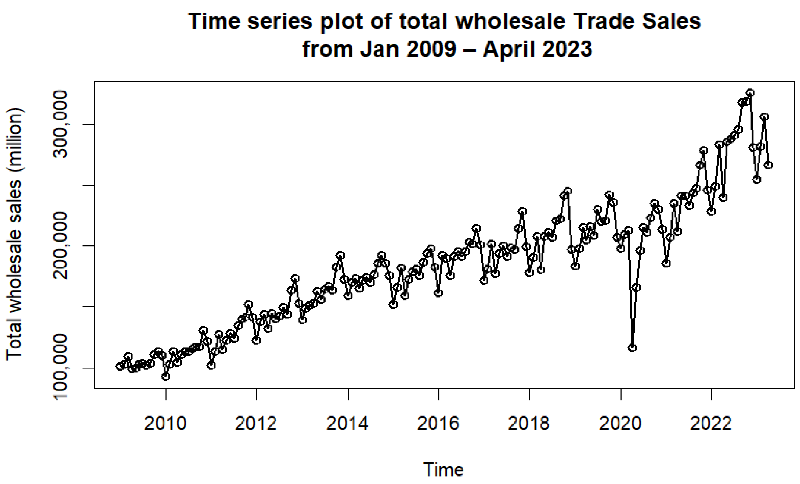
Figure 1. Time series plot of wholesale trade sales.
Economies 12 00249 g001
Figure 2. First and seasonally differenced wholesale trade sales series.
Economies 12 00249 g002
Figure 3. (a) Residual series plot, (b) ACF, and (c) histogram of standardised residuals from the SARIMA 2 , 1 , 1 0 , 1 , 1 12 model.
Economies 12 00249 g003
Figure 4. (a) Time series plot, (b) ACF and (c) histogram of standardised residuals of the SARIMA 2 , 1 , 1 0 , 1 , 1 12 model with the innovative outlier.
Economies 12 00249 g004
Figure 5. Time series plot of total retail trade sales ( R t ) from January 2009 to April 2023.
Economies 12 00249 g005
Figure 6. First and seasonally differenced inverse transformed total retail data pre-intervention.
Economies 12 00249 g006
Figure 7. (a) Residual series plot, (b) ACF and (c) histogram of standardised residuals from the SARIMA 0 , 1 , 1 0 , 1 , 0 12 model.
Economies 12 00249 g007
Figure 8. The impact of COVID-19 on the (a) wholesale and (b) retail trade sales from March 2020.
Economies 12 00249 g008
Figure 9. Resulting intervention impact models of (a) wholesale and (b) retail trade sales.
Economies 12 00249 g009
Figure 10. Quantifying the COVID-19 impact on (a) wholesale and (b) retail trade sales using pulse function by trial-and-error approach.
Economies 12 00249 g010aEconomies 12 00249 g010b
Figure 11. Capturing the COVID-19 impact on (a) wholesale and (b) retail trade sales using pulse function by fitted values/observed values approach.
Economies 12 00249 g011
Figure 12. Capturing the COVID-19 impact on (a) wholesale (b) trade sales using P t = 1 , where t = T 0 or 0 otherwise.
Economies 12 00249 g012
Figure 13. Estimated COVID-19 pandemic on the wholesale trade sales from March 2020 to May 2021.
Economies 12 00249 g013
Figure 14. Estimated COVID-19 pandemic on the retail trade sales from March 2020 to October 2020.
Economies 12 00249 g014
Table 1. SARIMA 2 , 1 , 1 0 , 1 , 1 12 model parameter estimates.
ParameterEstimateStandard ErrorTest Statisticp-Value
ϕ 1 −0.8687330.144873−5.99652.02   ×   10 9
ϕ 2 −0.5562780.081725−6.80689.98   ×   10 12
θ 1 0.3454270.1724632.00290.04519
Θ 1 −0.5303650.092548−5.73071.00   ×   10 8
Table 2. SARIMA 0 , 1 , 1 0 , 1 , 0 12 model parameter estimates.
ParameterEstimateStandard ErrorTest Statisticp-Value
θ 1 −0.8687330.144873−5.99652.02   ×   10 9
Table 3. AIC, BIC, RMSE, and MAPE for three approaches to fitting pulse functions to the wholesale series.
AICBICRMSEMAPE
Approach 1: Trial-and-Error2786.292803.774895.1731.887742
Approach 2: Fitted values/Observed values2848.312865.7915,312.135.697709
Approach 3: P t = 1 , if t = T 0 2909.662927.1323,184.319.750518
Table 4. Summary of COVID-19 estimated effects during 15 months of the intervention.
DateVector Covariates% ChangeEstimated COVID-19 Effect (Million)
Mar-2020−0.4−5.3%–ZAR 12,022
Apr-2020−3.0−43.4%–ZAR 91,017
May-2020−1.7−23.3%–ZAR 52,399
Jun-2020−0.4−7.2%–ZAR 16,054
Jul-2020−0.5−10.4%–ZAR 24,100
Aug-2020−0.3−6.9%–ZAR 15,867
Sep-20200.0−5.1%–ZAR 11,943
Oct-2020−0.3−5.6%–ZAR 14,060
Nov-2020−0.5−10.3%–ZAR 25,798
Dec-20200.0−3.5%–ZAR 7657
Jan-2021−0.6−12.2%–ZAR 25,160
Feb-20210.0−2.1%–ZAR 4598
Mar-20210.30.2%ZAR 454
Apr-20210.0−3.2%–ZAR 7087
May-20210.62.1%ZAR 4970
Total Effect–ZAR 302,339
Table 5. AIC, BIC, RMSE and MAPE for three approaches to fitting a pulse function for the Retail series.
AICBICRMSEMAPE
Approach 1: Trial-and-Error2225.672234.251106.460.8209
Approach 2: Fitted values/Observed values2423.742432.3210,141.9211.4421
Approach 3: P t = 1 , if t = T 0 2489.82498.3813,167.413.9439
Table 6. Summary of COVID-19 estimated effects during 8 months in the intervention period.
DateVector Covariates% ChangeEstimated COVID-19 Effect (Million)
Mar-20200.22.1%ZAR 1935
Apr-2020−4.5−48.1%−ZAR 43,534
May-2020−1.6−16.3%−ZAR 15,530
Jun-2020−1.0−9.5%−ZAR 8,866
Jul-2020−1.0−9.5%−ZAR 8744
Aug-2020−0.7−6.3%−ZAR 6073
Sep-2020−0.5−4.2%−ZAR 3966
Oct-2020−0.4−3.2%−ZAR 3058
Total Effect−ZAR 87,836
Disclaimer/Publisher’s Note: The statements, opinions and data contained in all publications are solely those of the individual author(s) and contributor(s) and not of MDPI and/or the editor(s). MDPI and/or the editor(s) disclaim responsibility for any injury to people or property resulting from any ideas, methods, instructions or products referred to in the content.