Inward Foreign Direct Investment and Trade Openness in Vietnam: A Nonlinear Autoregressive Distributed Lag Approach

Abstract

This study aims to examine the asymmetric relationship between trade openness and FDI (foreign direct investment) inflows to Vietnam by using NARDL (nonlinear autoregressive distributed lag) during the period from 1997 to 2019. Our findings show that the influence of FDI on trade openness is asymmetric in the short-run and long-run. But the influence of trade openness on FDI is symmetric in the short-run and asymmetric in the long run.

1. Introduction

Since the Government of Vietnam implemented the “Doi Moi” policy in 1986 and the Foreign Direct Investment Law in 1987, Vietnam’s economic growth has achieved remarkable development, so FDI has always played an essential role in Vietnam’s economy. Although some remarkable events are influencing the world economy such as the US-China trade war and the COVID-19 pandemic, the growth of FDI inflows to Vietnam has always remained relatively stable compared with others globally. According to the World Bank, Vietnam is one of the most attractive countries for FDI in Asia. On 24 January 2021, UNCTAD’s latest Global Investment Trends Monitor announced that global foreign direct investment (FDI) flows fell by 42% worldwide by 2020 compared to the data in 2019, but that figure significantly increased by 12% in East Asia. Furthermore, Vietnam has become the spotlight for foreign investors (UNCTAD 2020).

What makes Vietnam a destination for attracting foreign investors? The Vietnamese government has argued that tax rate reform and political stability are typical factors for attracting foreign investment. Some studies have realized that tax incentives preferences have completely positive effects on foreign investment in Vietnam and contributed to improving Vietnam’s comparative advantage in attracting FDI (Le 2004; Mai 2002; Yui 2006; Van 2019). In addition, political stability is important for foreign investors’ decision-making. Some studies stated that political stability is one of the dominant and necessary factors to create gravitation for foreign investors in Vietnam (Leung 2009; Ratnasingam and Ioras 2009; Delaunay and Torrisi 2012).

Numerous studies have pointed out that FDI is crucial to the impact and development of Vietnam’s economy. As a channel to increase capital, foreign direct investment has mainly had a major and positive impact on Vietnam’s economic growth (Anwar and Nguyen 2011; Thu et al. 2010). Jenkins (2006) argued that the influence of foreign direct investment on direct employment in Viet Nam has been remarkably restrained due to the high labor efficiency and the low ratio of value-added tax to the output of much of this investment. The impact of FDI also influences the labor form, workers’ living standards in Vietnam (McLaren and Yoo 2017), and the influence of FDI on Infrastructure Bottlenecks in Vietnam (Tran 2009). In order to boost FDI inflows, Vietnam needs to strengthen coordination and improve more policies, expand markets, and find new partners (Freeman 2002).

Most empirical studies on FDI in Vietnam rarely mention the relationship of the open door policy and foreign direct investment inflows into Vietnam. Theoretically, the effect of trade openness on the inflow of FDI varies according to the motivation for engaging in FDI activities (Dunning 1993; Markusen and Maskus 2002). Thus, this paper analyzes the role of trade openness in attracting FDI inflows to Vietnam in the endogenous growth theoretical framework. The research also uses annual data for the period 1997–2019. This current study further moved toward investigating regional macroeconomic fundamentals, which comprises trade openness, political stability, and tax rate impacts on Vietnam FDI inflow. The political stability and tax rate can both be considered as control variables to observe in this model.

Additionally, there has been empirical evidence of an asymmetric response of trade openness to foreign direct investment (Babatunde 2011). FDI inflows can help an economy by giving advantages for improving the level of the service sectors, consisting of telecommunications, banking and finance, transport, business and legal services, wholesale and retail trade. Therefore, in this study, we strive to assess the asymmetric influence of trade openness uncertainty on Vietnam’s FDI flows. It tests the concept that the more open developing markets are, the more attractive country’s FDI inflows will be.

Since few previous studies in Vietnam have particularly considered the asymmetric co-integration possibility and the long-term relationship between macroeconomics factors and FDI, this study will apply ARDL and the Nonlinear ARDL approaches as developed by Pesaran et al. (2001) and Shin et al. (2014) respectively, to examine short-term and long-term relationships and analyze the asymmetric effects between the variables.

In summary, this paper highlights the influence of macroeconomic factors on attracting foreign investment capital and the economy expansion in Vietnam. Regarding the ARDL and non-ARDL research methods, the authors will consider the correlation between FDI and the openness of the economy and examine the asymmetric influence of the two mentioned factors in the models with the rest of the macroeconomic factors. These methods also aim to identify a positive relationship between FDI and TO in the research model. This paper will help the Vietnam government and other developing countries create a foundation for balancing tax policies and political stability, thereby boosting economic openness and attracting more foreign direct investment.

2. Literature Review

2.1. Foreign Direct Investment

On a global scale, research has evinced that FDI plays a critical deterministic role in developing countries’ economies. Caves (1971) explained the direction of FDI investment in two ways: vertical and horizontal motivations. Horizontal FDI is a type of investment aimed at finding markets. The main goal of this type of investment is that foreign firms use some of the host country’s advantages to distribute products, sell products, and extend the life cycle of the business cycle. Meanwhile, vertical FDI is the type of investment aimed at finding resources. The main goal of this type of investment is to exploit raw materials, take advantage of the host country’s technologies, resources, and cheap labor costs to optimize costs as well as the production process of the product. Through the OLI (Ownership- Location-Internalization) framework, Dunning (1988) proved the determinant factors to FDI, which is related to three groups of advantages: advantage of ownership (O), advantage of Location (L), and advantage of Internalization (I). This article found that the aim of FDI into host countries is to minimize their cost of market research, tariff, and non-tariff barriers. Nunnenkamp (2002) studies the determinants of FDI in developing countries in the context of globalization. The results show that globalization has a significant effect on FDI. Therefore, non-traditional factors gradually become more critical to FDI attraction, such as costs, additional production factors, as well as economy openness. Meanwhile, traditional factors such as market size and growth rate decrease slightly in the impact of FDI inflow.

Many empirical studies related to factors affecting FDI by different methods. Demirhan and Masca (2008) identified the factors affecting FDI in 38 developing countries 2000–2004, using a cross-data analysis model, including size market; inflation rate; the infrastructure; labor costs; economy openness; political risks, and tax rate. The result also showed that the above factors all positively affect FDI attraction, except for labor costs and political risks. Jayasekara (2014) accomplished the determinants of FDI in Sri Lanka, India, Bangladesh, and Pakistan from 1975 to 2012, applying the modified smallest regression model (FM-OLS). The factors included in the analysis model include, GDP growth rate representing market size, the inflation rate, government spending, exchange rates represent macroeconomic stability, the loan interest rate for financial development, the total value of imports and exports representing the openness of the economy, workforce, and the number of telephone lines per 100 people in the country representing infrastructure. The results show that there are positive effects on GDP growth, government spending, total exports and imports, workforce, and infrastructure. However, inflation, exchange rate, and interest rates negatively affect the FDI attraction and competition among countries. In addition, the study has shown that by adding tariffs on international trade, the country’s socio-economic conditions also affect FDI inflows. McLean and Shrestha (2002) determine that FDI plays a more essential role in economic growth of developing countries than developed nations.

2.2. Trade Openness

Goldberg and Klein (1998) indicate that FDI promotes more significant trade in exports, import substitution, or intermediate inputs. Trade openness prompts export-oriented FDI, while trade restrictions appeal for “tariff jump” FDI, the primary goal of taking advantage of the domestic market (Liargovas and Skandalis 2012). At the same time, the literature on trade liberalization shows that liberalization promotes domestic investment by accepting domestic agents to import relatively cheap and more efficient capital products, thereby reducing structural constraints on investment and increasing the efficiency of capital accumulation (Kosteletou and Liargovas 2000). Similarly, some transnational studies have concluded that foreign direct investment can only promote economic growth if the host country’s trade openness is sufficiently high (Lee 1995).

In other terms, Markusen and Maskus (2002) point out that the relationship between trade openness and FDI inflows is very complicated and needs to be carefully explained, possibly depending on the characteristics of each case. In theory, the impact of trade openness on FDI inflows varies with the motivation for engaging in FDI activities. Makoni (2018) and Zaman et al. (2018) found a positive relationship between trade openness and FDI inflows; Khan and Hye (2014); Adow and Tahmad (2018); Cantah et al. (2018) and Rathnayaka Mudiyanselage et al. (2021) found a negative relationship; while Ho et al. (2013) and Wickramarachchi (2019) found that trade openness had no significant impact on FDI inflows.

2.3. Political Stability

On the other hand, economic growth and political stability are closely related; thus, political stability is also the decisive factor for a multinational company to make new investment decisions. According to empirical studies, FDI inflows are influenced by the political stability index of the host country (La Porta et al. 1999; Kim 2010; Shahzad and Al-Swidi 2013), with such research as Akin (2019) also further explains that foreign companies usually consider low labor costs or commodity resources, and low taxes, political stability, economic freedom, and current free trade of the host country in order to make their final investment decisions. Contrary to opinions about the support of political stability factor positively affecting FDI, the empirical evidence of Kurecic and Kokotovic (2017) suggested that political stability did not produce a statistically significant impact on foreign investors, being only an initial condition for beginning investment in smaller economies as developing countries.

2.4. Tax Rate

Furthermore, a very key contribution by Scholes and Wolfson (1990) and Cassou (1997) using a panel methodology, determined a significant negative relationship between FDI inflow and corporate tax rate, pointing out that host country corporate income tax rates have a significant effect on the inflow of investment. Scholes and Wolfson (1990) argued that it is definitely possible for overseas investors to improve their own investment in response to higher US corporate taxes. Some empirical analysis also pointed out that tax incentives have a significant impact on FDI decision-making (Tung and Cho 2000; Hsu et al. 2019; Etim et al. 2019; Siregar and Patunru 2021). The rates of tax can either positively or negatively affect the inflow of foreign direct investments (FDIs) in a country, due to the taxation system of the host country (Ojeka et al. 2021).

3. Data Sources and Description of Variable

3.1. Data

Time series data per annum on FDI, trade openness, tax, and political stability covering the 1997–2019 period has been used in this study. Data were collected and aggregated from various sources, namely World Bank data, and annual reports by the general statistics office of Vietnam.

The data of foreign direct investment inflow (FDI) and political stability (PS) variables are completely gathered from World Bank source. Trade openness (TO) is measured by the total sum of exports and imports divided by GDP. Because of drawing attention to foreign investment capital, the Vietnamese government has consecutively changed corporate income tax rate. Before 1999, the government did apply a corporate tax rate of 25% to FDI enterprises. In 2003, the Law on Corporate Income Tax underwent major reform when it unified tax obligations, and tax incentives between domestic enterprises and FDI enterprises at the same rate became 28%. In the period 2009–2015, the corporate tax for FDI companies was 25%; after 2016, this rate declined to 20%. In addition, the government also applied a tax rate to transferring profits overseas with rates of 5% to 10% for the period before 2000, and after 2000 at 3% to 7%. Therefore, the actual corporate income tax for FDI companies will be calculated as corporate income tax plus tax on repatriation of profits abroad.

For experimental design, descriptive statistics (mean, median, standard deviation, skewness, and kurtosis) were used in the calculation to check the nature of the data distribution. The Jarque Bera test determines the normal distribution of the data. Based on the description statistic in

Table 1. Result of description.

	TO	TAX	FDI	PS
Mean	147.525	0.302	6.64 × 109	0.255
Median	152.217	0.303	7.43 × 109	0.252
Maximum	210.400	0.330	1.61 × 1010	0.526
Minimum	94.344	0.256	1.30 × 109	−0.022
Std. Dev.	34.514	0.027	5.05 × 109	0.137
Skewness	0.238	−0.623	0.410	0.114
Kurtosis	2.126	2.070	1.883	2.455
Jarque-Bera	0.948	2.315	1.839	0.335
Probability	0.622	0.314	0.399	0.846
Sum	3393.065	6.945	1.53 × 1022	5.858
Sum Sq. Dev.	26,210.57	0.016	5.61 × 1020	0.412

, most of the variables are left deviations (positively skewed) except for the tax. For Kurtosis method measuring the peakness or flatness of the distribution of the analyzed series, all variables are platykurtic. After analyzing the goodness-of-fit test, the probability of TO, TAX, FDI, PS has statistical meaning. Thus, according to the Jarque-Bera statistic, the time series data matches a normal distribution.

3.2. Unit Root Test

The purpose of the unit root test is to examine whether the data is stationary or not. Thus, this paper used ADF and Phillips-Perron tests. According to Dickey and Fuller (1981) the time series attributes of each research variable that are studied for unit roots are studied through the enhanced Augmented Dickey-Fuller test (ADF). The Phillips-Perron (PP) test is also used to confirm the ADF test (Phillips and Perron 1988) Estimate the common equality of ADF and PP tests according to the following formula:

$$\Delta Y_t=C_0+{\alpha }_1{Y}_{t-1}+{\alpha }_{2}t+{{\displaystyle \sum }}_{j=1}^n{r}_j\Delta Y_{t-j}+{\epsilon }_t$$

$$\Delta Y_t=C_0+{\alpha }_1{Y}_{t-1}+{\alpha }_{2}t+{\epsilon }_t$$

Among them: Y is a time series, t is a linear time trend, ∆ is the first difference operator, which is a constant, n is the optimal number of lags in the dependent variable, and ${\epsilon }_t$ is a random error term.

• The null hypothesis (H1). that the time series is not stationary (with unit root).
• The alternative hypothesis (H2). that the time series is stationary (no unit root).

If the calculated test statistic is less than the critical value of the test statistic, then the null Hypothesis (H1) will be rejected. Unit root test result reports in

Table 2. Unit root test result.

Variable	ADF				PP
At Level
	None	Intercept	Trend and Intercept	I	None	Intercept	Trend and Intercept	I
LNFDI	1.637 (0.971)	−0.114 (0.936)	−2.559 (0.299)	-	1.418 (0.9562)	−0.281 (0.913)	−2.528 (0.3129)	-
LNTO	4.674 (1.000)	−0.694 (0.827)	−1.983 (0.5746)	-	6.604 (1.000)	−0.838 (0.788)	−3.145 (0.121)	-
LNTAX	1.263 (0.942)	−0.358 (0.900)	−1.675 (0.727)	-	1.331 (0.949)	−0.312 (0.908)	−1.677 (0.727)	-
LNPS	−1.033 (0.261)	−2.942 ** (0.060)	−5.305 *** (0.003)	I(0)	−2.695 *** (0.009)	−5.423 *** (0.001)	−5.289 *** (0.002)	I(0)
At First Difference
LNFDI	−2.955 *** (0.005)	−3.321 *** (0.007)	−3.160 (0.119)	I(1)	−2.925 *** (0.005)	−3.260 ** (0.030)	−3.070 * (0.102)	I(1)
LNTO	−0.745 (0.379)	−6.669 *** (0.000)	−6.540 *** (0.000)	I(1)	−3.882 *** (0.000)	−7.461 *** (0.000)	−7.594 *** (0.000)	I(1)
LNTAX	−4.472 *** (0.000)	−4.741 *** (0.000)	−4.771 *** (0.001)	I(1)	−4.487 *** (0.000)	−4.741 *** (0.001)	−4.771 ** (0.005)	I(1)
LNPS	−6.089 *** (0.000)	−3.612 ** (0.020)	−3.694 * (0.058)	I(1)	−21.050 *** (0.000)	−22.560 *** (0.000)	−22.857 *** (0.000)	I(1)

Note: 1. Table 2 shows values of t-statistics and p-values in parentheses. 2. ***, ** and * indicate significance at 1%, 5%, and 10% levels. 3. None, Intercept, Trend, and Intercept are conditions of unit root test. 4. Symbol “I” indicates an order of integration.

. According to the ADF and Phillips-Perron tests, results indicate that only LNPS is stationary at I(0), and all variables are stationary after the first difference, with at least 2 out of 3 conditions being met (none, intercept, trend and intercept). The ARDL and NARDL models, developed by Pesaran et al. (2001) and Shin et al. (2014) allow for simultaneous analysis for both short-term and long-term asymmetric effects between variables, regardless of the static variables at I(0) or I(1) (Ding et al. 2017); therefore, a unit root test is performed to ensure that the variable is not stationary at I(2).

3.3. Methodology

After examining the unit root test, the authors continued to conduct the data analysis process based on the primary method, the autoregression distribution lag model (ARDL), to determine the relationship between endogenous variables (FDI, TO) and exogenous variables (PS, TAX) in the short and long term. Following that, to observe the nexus between endogenous variables (FDI and TO) more clearly, we continued to use the non-linear ARDL method to analyze the asymmetric effect between them in the analytical model.

Consequently, the authors used regression diagnostics test to evaluate the variables in the selected model as to whether or not there was a large undue influence on the analysis. Breusch–Godfrey test, Harvey test, and Jarque-Bera test were used for assessing assumptions; cumulative sum (CUSUM) and CUSUM of squares (CUSUMSQ) tests were used for assessing the structure stability.

3.4. The Model

This study indicated the impact of macroeconomic factors on foreign direct investment and trade openness, based on endogenous growth theory, and followed Ding et al. (2017) a study based on the following equation:

$$FDI=f\left(TO; TAX, PS\right)$$

(1)

$$TO=f\left(FDI ;TAX, PS\right)$$

(2)

After changing it into a linear form, Equations (1) and (2) can be considered as the following step:

$$LNFDI=\alpha +{\delta }_1^{}LNTO+{\delta }_2^{} LNTAX+{\delta }_3^{}LNPS+{\epsilon }_t^{}$$

(3)

$$LNTO=\beta +{\lambda }_1^{}LNFDI+{\lambda }_2^{} LNTAX+{\lambda }_3^{}LNPS+{\rho }_t^{}$$

(4)

where:

• $LN$: represents the logarithm.
• $LNFDI$: the logarithm of the foreign direct investment.
• $LNTO$: the logarithm of the trade openness.
• $LNTAX$: the logarithm of the tax rate.
• $LNPS$: the logarithm of the political stability.

Moreover, Equations (3) and (4) showed that $\delta$₁ to $\delta$₃, ${\lambda }_1^{}$ to ${\lambda }_3^{}$ coefficients correspond to long-term elasticities, ${\epsilon }_t^{}$ and ${\rho }_t^{}$ stands for the random remainder of the estimated regression.

3.4.1. ARDL Model

This study has used autoregressive distributed lag (ARDL), proposed by Pesaran et al. (2001), to define the impact of long-run and short-run associations between the variables of interest (FDI, trade openness, tax, political stability) due to the following benefits. The ARDL model is carried out in the following sequence: First, the co-integration between the variables are analyzed by the Bound test, which helped to determine the long-run relationship between the variables; second, determining the lags of the variables, which used the SBC or AIC criteria; third, running the ARDL model with the defined lags to test the long-run relationship between the variables in the model; and subsequently calculating the short-term effects of variables by error correction model (ECM), based on the ARDL approach to defining the co-integration relationship between the observed variables.

According to Pesaran et al. (2001), the ARDL method has several dominances over other co-integration methods: First, in the case of small sample sizes, the ARDL model is the more statistically significant approach, aiming to test for co-integration, while that of the Johansen’s co-integration technique requires a larger number of samples to achieve reliability; secondly, in contrast to conventional methods for finding long-run relationships, the ARDL method does not estimate a system of equations; thirdly, other co-integration techniques require that the regressors are included in the association with the same delay whereas in the ARDL approach, the regressors can tolerate different optimal lags; and subsequently, if the author does not guarantee the properties of the unit root or the stationarity of the data system, the association level I(1) or I(0), the application of ARDL is the most appropriate for the study experiment.

The ARDL model is defined as follows:

$$\begin{array}{ll}\Delta LNFD{I}_{t,i}& ={\alpha }_1+{{\displaystyle \sum }}_{i=1}^m{\mathsf{\mu }}_{1i}\Delta LNFD{I}_{t-i}+{{\displaystyle \sum }}_{i=0}^n{\mathsf{\mu }}_{2i}\Delta LNT{O}_{t-i}\\ & +{{\displaystyle \sum }}_{i=0}^k{\mathsf{\mu }}_{3i}\Delta LNTA{X}_{t-i}+{{\displaystyle \sum }}_{i=0}^r{\mathsf{\mu }}_{4i}\Delta LNP{S}_{t-i}\\ & +{\mathsf{\gamma }}_{1}LNFD{I}_{t-1}+{\mathsf{\gamma }}_{2}LNT{O}_{t-1}+{\mathsf{{\rm Y}}}_{3}LNTA{X}_{t-1}+{\mathsf{{\rm Y}}}_{4}LNP{S}_{t-1}+{\omega }_t\end{array}$$

(5)

$$\begin{array}{ll}\Delta LNT{O}_{t,i}& ={\alpha }_2+{{\displaystyle \sum }}_{i=0}^m{\theta }_{1i}\Delta LNFD{I}_{t-i}+{{\displaystyle \sum }}_{i=1}^n{\theta }_{2i}\Delta LNT{O}_{t-i}\\ & +{{\displaystyle \sum }}_{i=0}^k{\theta }_{3i}\Delta LNTA{X}_{t-i}+{{\displaystyle \sum }}_{i=0}^r{\theta }_{4i}\Delta LNP{S}_{t-i}\\ & +{\pi }_{1}LNFD{I}_{t-1}+{\pi }_{2}LNT{O}_{t-1}+{\pi }_{3}LNTA{X}_{t-1}+{\pi }_{4}LNP{S}_{t-1}+{\theta }_t\end{array}$$

(6)

where $\mu$ and $\theta$ are short-run coefficients. $\gamma$ and $\pi$ are the long-run coefficients. The symbol $\Delta$ denotes the first differences of the variables, while m, n, k, r represents the lags of the variables.

Bound test, mainly based on the F statistic to test the co-integration between observed variables. Accordingly, Pesaran et al. (2001) and Qamruzzaman et al. (2019) have provided more concrete evidence to demonstrate the co-integration relationship in the long-run model. Thus, these tests aim to define the long-run relationship that exists among these elements by handling an F-test with the hypotheses:

-

Hypothesis H1: $\left[\begin{array}{c}{\gamma }_1={\gamma }_2={\gamma }_3={\gamma }_4\\ {\pi }_1={\pi }_2={\pi }_3={\pi }_4\end{array}\right]=0$ there is no co-integration relationship between variables;

-

Hypothesis H2: $\left[\begin{array}{c}{\gamma }_1\ne {\gamma }_2\ne {\gamma }_3\ne {\gamma }_4\\ {\pi }_1\ne {\pi }_2\ne {\pi }_3\ne {\pi }_4\end{array}\right]\ne 0$ a co-integration relationship exists between variables.

The null hypothesis is rejected when the value of the F-statistic is larger than the upper critical bounds value, and it is not rejected if this value is lower than the lower bounds value. Contrariwise, when the nexus of co-integration between these variables is indeterminate, the error correction model (ECM) is implemented to identify co-integration relationship. If the estimated coefficient is significant, it has sufficient evidence to conclude that the co-integration nexus between variables is available (Bahmani-Oskooee and Fariditavana 2015).

Once the result indicates that co-integration relationship between these variables is present, it means that a long-run relationship between them exists in the model. The long-run ARDL model is expressed as follows:

$$\begin{gathered} \Delta LNFD{I}_{t,i}={\alpha }_1+{{\displaystyle \sum }}_{i=1}^m{\mathsf{\mu }}_{1i}\Delta LNFD{I}_{t-i}+{{\displaystyle \sum }}_{i=0}^n{\mathsf{\mu }}_{2i}\Delta LNT{O}_{t-i}+{{\displaystyle \sum }}_{i=0}^k{\mathsf{\mu }}_{3i}\Delta LNTA{X}_{t-i} \\ +{{\displaystyle \sum }}_{i=0}^r{\mathsf{\mu }}_{4i}\Delta LNP{S}_{t-i}+\psi EC{T}_{t-i}+{\omega }_{1t} \end{gathered}$$

(7)

$$\begin{array}{ll}\Delta LNT{O}_{t,i}& ={\alpha }_2+{{\displaystyle \sum }}_{i=0}^m{\theta }_{1i}\Delta LNFD{I}_{t-i}+{{\displaystyle \sum }}_{i=1}^n{\theta }_{2i}\Delta LNT{O}_{t-i}+{{\displaystyle \sum }}_{i=0}^k{\theta }_{3i}\Delta LNTA{X}_{t-i}\\ & +{{\displaystyle \sum }}_{i=0}^r{\theta }_{4i}\Delta LNP{S}_{t-i}+\varphi EC{T}_{t-i}+{\omega }_{2t}\end{array}$$

(8)

Estimating the short-term coefficients of the ARDL model followed by the error correction model (ECM) with selected lag length. The error correction model is presented as follows:

$$EC{T}_{1t}=LNFD{I}_{t-1}-\frac{{\mathsf{\gamma }}_2}{{\mathsf{\gamma }}_1}LNT{O}_{t-1}-\frac{{\mathsf{\gamma }}_3}{{\mathsf{\gamma }}_1}LNTA{X}_{t-1}-\frac{{\mathsf{\gamma }}_4}{{\mathsf{\gamma }}_1}LNP{S}_{t-1}$$

(9)

$$EC{T}_{2t}=LNT{O}_{t-1}-\frac{{\pi }_1}{{\pi }_2}LNFD{I}_{t-1}-\frac{{\pi }_3}{{\pi }_2}LNTA{X}_{t-1}-\frac{{\pi }_4}{{\pi }_2}LNP{S}_{t-1}$$

(10)

3.4.2. Non-Linear Autoregressive Distributed Lagged (NARDL)

The notion of nonlinearity among dependent and explanatory variables has recently become one of the significant aspects when evaluating relationships in empirical investigations. When it comes to nonlinearity, Shin et al. (2014) proposed a new non-linear co-integration equation, which has become generally known as a NARDL by combining two sets of additional explanatory variables in the equation: positive and negative shocks. More importantly, we can use Equations (8) and (9) below to estimate the level of positive and negative shocks in explanatory variables.

$$\{\begin{array}{c}FD{I}_t^{+}={{\displaystyle \sum }}_{i=1}^{t}LNFD{I}_i^{+}={{\displaystyle \sum }}_{i=1}^{t}MAX\left(\mathsf{\Delta }LNFD{I}_k,0\right)\\ FD{I}_t^{-}={{\displaystyle \sum }}_{i=1}^{t}LNFD{I}_i^{-}={{\displaystyle \sum }}_{i=1}^{t}MIN\left(\mathsf{\Delta }LNFD{I}_k,0\right)\end{array}$$

(11)

$$\{\begin{array}{c}T{O}_t^{+}={{\displaystyle \sum }}_{i=1}^{t}LNT{O}_i^{+}={{\displaystyle \sum }}_{i=1}^{t}MAX\left(\mathsf{\Delta }LNT{O}_k,0\right)\\ T{O}_t^{-}={{\displaystyle \sum }}_{i=1}^{t}LNT{O}_i^{-}={{\displaystyle \sum }}_{i=1}^{t}MIN\left(\mathsf{\Delta }LNT{O}_k,0\right)\end{array}$$

(12)

Thus, the asymmetric relationship between FDI and TO is estimated by the following equation:

$$\begin{array}{ll}\Delta LNFD{I}_{t,i}& ={\alpha }_0+{{\displaystyle \sum }}_{i=1}^m{\mathsf{\mu }}_{1i}\Delta LNFD{I}_{t-i}+{{\displaystyle \sum }}_{i=0}^n{\mathsf{\mu }}_{2i}^{+}\Delta LNT{O}_{t-i}^{+}+{{\displaystyle \sum }}_{i=0}^n{\mathsf{\mu }}_{2i}^{-}\Delta LNT{O}_{t-i}^{-}\\ & +{{\displaystyle \sum }}_{i=1}^k{\mathsf{\mu }}_{3i}\Delta LNTA{X}_{t-i}+{{\displaystyle \sum }}_{i=0}^r{\mu }_{4i}LNP{S}_{t-i}+{\mathsf{{\rm Y}}}_{1}LNFD{I}_{t-1}\\ & +{\mathsf{{\rm Y}}}_2^{+}LNT{O}_{t-1}^{+}+{\mathsf{{\rm Y}}}_2^{-}LNT{O}_{t-1}^{-}+{\mathsf{{\rm Y}}}_{3}LNTA{X}_{t-1}+{\mathsf{{\rm Y}}}_{4}LNP{S}_{t-1}+{\omega }_{1t}\end{array}$$

(13)

$$\begin{array}{ll}\Delta LNT{O}_{t,i}& ={\alpha }_0+{{\displaystyle \sum }}_{i=0}^m{\theta }_{1i}^{+}\Delta LNFD{I}_{t-i}^{+}+{{\displaystyle \sum }}_{i=0}^m{\theta }_{1i}^{-}\Delta LNFD{I}_{t-i}^{-}+{{\displaystyle \sum }}_{i=1}^n{\theta }_{2i}\Delta LNT{O}_{t-i}\\ & +{{\displaystyle \sum }}_{i=1}^k{\theta }_{3i}\Delta LNTA{X}_{t-i}+{{\displaystyle \sum }}_{i=0}^r{\theta }_{4i}LNP{S}_{t-i}+{\mathsf{\pi }}_1^{+}LNFD{I}_{t-1}^{+}\\ & +{\pi }_1^{-}LNFD{I}_{t-1}^{-}+{\mathsf{\pi }}_{2}LNT{O}_{t-1}+{\pi }_{3}LNTA{X}_{t-1}+{\mathsf{\pi }}_{4}LNP{S}_{t-1}+{\omega }_{2t}\end{array}$$

(14)

Empirical analysis proceeds in the following three steps: First, Equations (12) and (13) is estimated by the method of least squares (OLS). Step two, null hypothesis H1: There is no long-run relationship between variables (H1: $\left[\begin{array}{c}{\gamma }_1={\gamma }_2^{-}={\gamma }_2^{+}={\gamma }_3={\gamma }_4\\ {\pi }_1^{+}={\pi }_1^{-}={\pi }_2={\pi }_3={\pi }_4\end{array}\right]$ = 0) is tested based on the F-statistics (Pesaran et al. 2001; Shin et al. 2014).

Finally, short-run and long-run asymmetry tests are performed based on the Wald test:$H_{LR}$: $\left|\begin{array}{cc}{\gamma }_2^{+}/{\gamma }_1 =& {\gamma }_2^{-}/{\gamma }_1\\ {\pi }_1^{+}/{\pi }_2=& {\pi }_1^{-}/{\pi }_2\end{array}\right|$, or $H_{SR}:$ $\left|\begin{array}{cc}{{\displaystyle \sum }}_{i=0}^n{\mathsf{\mu }}_{2i}^{+}=& {{\displaystyle \sum }}_{i=0}^n{\mathsf{\mu }}_{2i}^{-}\\ {{\displaystyle \sum }}_{i=0}^m{\theta }_{1i}^{+}=& {{\displaystyle \sum }}_{i=0}^m{\theta }_{1i}^{-}\end{array}\right|$

If only the $H_{SR}$ hypothesis: $\left|\begin{array}{cc}{{\displaystyle \sum }}_{i=0}^n{\mathsf{\mu }}_{2i}^{+}=& {{\displaystyle \sum }}_{i=0}^n{\mathsf{\mu }}_{2i}^{-}\\ {{\displaystyle \sum }}_{i=0}^m{\theta }_{1i}^{+}=& {{\displaystyle \sum }}_{i=0}^m{\theta }_{1i}^{-}\end{array}\right|$ is rejected, then this model is asymmetric in the short-run.

If only the $H_{LR}$ hypothesis: $\left|\begin{array}{cc}{\gamma }_2^{+}/{\gamma }_1=& {\gamma }_2^{-}/{\gamma }_1\\ {\pi }_1^{+}/{\pi }_2=& {\pi }_1^{-}/{\pi }_2\end{array}\right|$ is rejected, then this model is asymmetric in the long-run.

If both hypotheses $H_{LR}$:$\left|\begin{array}{cc}{\gamma }_2^{+}/{\gamma }_1=& {\gamma }_2^{-}/{\gamma }_1\\ {\pi }_1^{+}/{\pi }_2=& {\pi }_1^{-}/{\pi }_2\end{array}\right|$ and $H_{SR}:$ $\left|\begin{array}{cc}{{\displaystyle \sum }}_{i=0}^m{\mathsf{\mu }}_{1i}^{+}=& {{\displaystyle \sum }}_{i=0}^m{\mathsf{\mu }}_{1i}^{-}\\ {{\displaystyle \sum }}_{i=0}^n{\theta }_{2i}^{+}=& {{\displaystyle \sum }}_{i=0}^n{\theta }_{2i}^{-}\end{array}\right|$ are not rejected, Equations (13) and (14) reduce to linear form in the short-run and the long-run, which is exactly the traditional ARDL model of Pesaran et al. (2001).

4. Results

4.1. Optimal Lag Length

Before examining the existence of a long-run relationship between variables based on the co-integration test, the study determined the optimal lag length based on the VAR model with the original data. The number of observations was limited with one lag maximum because the observed data are annual time series.

The results in

Table 3. The optimal number of lags results.

Lag	LogL	LR	FPE	AIC	SC	HQ
0	−8.772155	NA	3.97 × 10−5	1.216396	1.415352	1.259574
1	63.7986	110.5840 *	1.88 × 10−7 *	−4.1713 *	−3.1765 *	−3.9554 *
2	72.2299	9.6359	4.72 × 10−7	−3.4505	−1.6597	−3.062

Note: * indicates the optimal number of lags.

are obtained for the criteria FPE, AIC, and HQ. The optimal number of lags in the model is one.

4.2. Results of ARDL

4.2.1. The Bound Test and the Long-Run Dynamic Model

The purpose of the bound test is to check whether a co-integration relationship exists or not. If the value of F-statistics exceeds the upper critical bound I(1), the null hypothesis of no co-integration is rejected. Otherwise, if this value does not pass the lower critical bound I(0), then no co-integration relationship exists between observed variables. On the one hand, the results in

Table 4. Autoregressive distribution lag model result.

Model 1 LNFDI as the Dependent Variable Selected Model: ARDL(1, 0, 1, 1)			Model 2 LNTO as the Dependent Variable Selected Model: ARDL(1, 1, 1, 0)
(a) The Long-Run Relation Model
Variables	Coefficients	t-Statistics	Variables	Coefficients	t-Statistics
C	−1.115	−1.268	C	0.275	1.361
LNTO	6.732 ***	8.854	LNFDI	0.122 ***	3.619
LNTAX	7.3367 ***	3.896	LNTAX	−1.399 ***	−3.850
LNPS	−0.097	−1.393	LNPS	0.032	1.587
F-Bound Test	11.911 (Co-integration)		F-Bound Test	5.083 (Inconclusive )
ECM	--		ECM	−0.406 *** (Co-integration)
Critical value at 1% level of significance	I(0) 4.29	I(1) 5.61	Critical value at 2.5% level of significance	I(0) 3.25	I(1) 4.49
(b) Short-Run Dynamic ECT Model
ECT (−1)	−0.426 ***	−6.454	ECT (−1)	−0.406 ***	−4.821
$\Delta$(LNTO)	3.041 ***	4.345	$\Delta$(LNFDI)	0.162 ***	4.401
$\Delta$(LNTAX)	−1.095	−1.129	$\Delta$(LNTAX)	0.506 **	2.456
$\Delta$(LNPS)	−0.045 **	−2.259	$\Delta$(LNPS)	0.0144 **	2.835
(c) Diagnostic Test
R-squared	0.981		R-squared	0.981
F-statistic	132.866 ***		F-statistic	135.975 ***
Breusch-Godfrey	${\chi }_{}^2$ = 2.922		Breusch-Godfrey	${\chi }_{}^2$ = 8.157 **
Harvey	${\chi }_{}^2$ = 11.972		Harvey	${\chi }_{}^2$ = 11.498 *
Jarque-Bera	${\chi }_{}^2$ = 9.608 ***		Jarque-Bera	${\chi }_{}^2$ = 0.435

Note: ***, **, * indicate significant levels at 1%, 5%, 10% respectively.

a indicate that when FDI is considered as a dependent variable, the F-statistics is 11.910, which is much higher than I(1), meaning that the null hypothesis of no co-integration is rejected. On the other hand, when trade openness is considered as a dependent variable, the F-statistics is 5.083 which falls between the lower and upper critical values at 1% significant level, but the F statistics value of trade openness exceeded the upper value at 2.5% significant level. To identify the existence of co-integration relationship among these variables visibly, the error correction model (ECM) can also be applied. The coefficient of ECT(−1) is −0.406 (p = 0.000), which is significant at 1%; thus, this is evidence for the co-integration among these variables (Bahmani-Oskooee and Fariditavana 2015). Accordingly, the results in Table 4a imply that there is a long-run relationship among all variables, even if trade openness or FDI is considered as dependent variables.

Based on the results in Table 4a shown above, it is clear that there is a significantly positive effect of trade openness on FDI in the long-term valuation when FDI is considered the dependent variable. Especially, a rise in the level of trade openness by one unit, results in an increase in FDI inflows by 6.732 units. Similarly, when FDI increases, it will lead to an increase in trade openness. In contrast, tax policies still seem to play an essential role in the model, and the rate of tax will be opposite to both dependent variables. The increase in taxation has led to an increase in FDI, which is not in line with expectations. However, the increase in taxation has led to a decrease in the degree of trade openness, mainly due to the high value-added tax and income tax burden that has led to the substitution of trade for production in Vietnam. Political stability does not significantly affect FDI and trade openness in the long run.

4.2.2. The Short-Run Dynamic Model

The result of short-run estimation is represented in Table 4b. The error correction term (ECT(−1) = −0.426, ECT(−1) = −0.407) is negative and at significant level within 1% in both cases, indicating the short-run adjustment among trade openness and FDI inflows is present, also implying that there is a high-speed adjustment to a long-term equilibrium under the impact of trade openness and FDI inflows in the last year. Meanwhile, in the short term, the tax rate has no significant effect on FDI, but substantially affects the trade openness at 5% significant level. When trade openness can be seen as the dependent variable, FDI inflow total impacts on the trade openness are significant but inelastic (with the coefficient of 0.163) in the short period.

Generally, when FDI is considered a dependent variable, most of the independent variables significantly affect the FDI inflows in the short-run except for the tax rate. The tax rate has no effect on foreign investors’ decisions in the short-run, but it significantly affects FDI in the long-run. In contrast, it seems that foreign investors who want to invest in the short run are very interested in Vietnam’s political stability. Still, in the long-run, they overlook the political situation. Meanwhile, Model 2 shows the sensitivity of TO in both short-run and long-run when all experimental factors impose their effects, except for PS in the long-run period. Thus, we can conclude that the trade openness is affected by factors such as FDI capital, tax rate, and short-run political stability.

4.2.3. Diagnostic Test

More importantly, we conducted a diagnostic test in Table 4c aimed at testing variables. The result of R squared of both models is 0.981, which means that these observed variables can strongly explain the relationship between each other, and the experimental model has high reliability. The F-test of overall significance indicates that our models distribute a good fit for the data. For the residual test, we applied the Harvey test of heteroscedasticity, Breusch-Godfrey Serial Correlation, and the Jarque-Bera-normality test. Then, we implemented the Ramsey RESET, CUSUM and CUSUM SQUARE in the stability test. The value of observations R-square was used to measure the results of the diagnostic tests (including Harvey, Breusch-Godfrey, Jarque-Bera, Ramsey RESET).

More particularly, the Breusch-Godfrey test was used to determine the serial correlation between variables, and the evidence indicated that variables only reflect correlation in Model 2. The null hypothesis of no autocorrelation can be rejected at a 5% level of significance but not at 1% level. In general, the lag can be increased to solve the sequence correlation problem; however, due to the short period of data, the estimation results are still credible (Bahmani-Oskooee et al. 2019). The Harvey test for the null hypothesis of no heteroskedasticity can be rejected at 10% level of significance but not at 5%. We can conclude that the problem of serial correlation and heteroskedasticity of this estimation model is not serious.

For the Jarque-Bera normality test, the residual R-squared value is not significant in Model 2, indicating that these residual distributions are normally distributed in the model. In contrast, the Jarque-Bera value in Model 1 is significant at the 1% level of significance, and there is a normality problem.

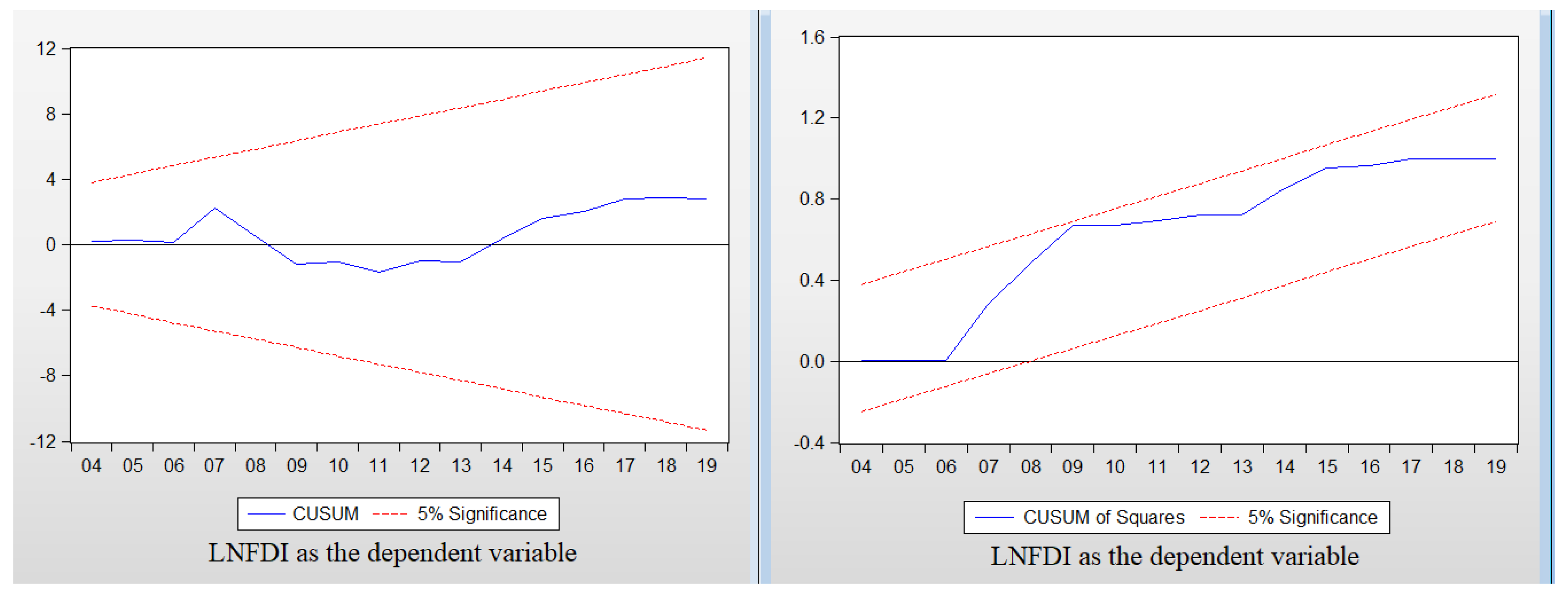
Subsequently, the CUSUM and CUSUM of squares is used for examining the residual instability and structural variation. The graph in Figure 1 illustrates that most of the blue line is not out of bounds except for CUSUM of Squares when LNTO is considered as an independent variable, which marginally surpassed the two red bounds. According to Abdlaziz et al. (2016) and Kim (2017) this evidence indicates that the experimental models still remain reliable and significantly statistical. From the paragraph in Figure 1, the accumulation of repeated residues falls within the boundary of the critical zone, confirming the stability of the model at a significance level of 5%, so it can be said that the long-run and short-run outcomes of the estimated model is congruent and stable, so it can be concluded that the collected data are stable and the estimated results are reliable, and can therefore be used for further analysis and prediction.

4.3. Results of NARDL

To test the asymmetric effect between FDI and Trade openness, the authors conducted regression of two NARDL models, including Model 3—NARDL (1, 1, 0, 1, 1) that aimed to test the asymmetry of Trade openness on FDI and Model 4—NARDL (1, 2, 2, 2, 2) to test short asymmetry of FDI on trade openness. The purpose of dividing into two factors (positive and negative) is to observe the interaction of FDI and trade openness to experiment with the relationship between them in the analytical models. Therefore, there is a difference in the number of variables in these models. Still, the significance of the impact between the remaining variables (political stability and tax rate) remains unchanged. Based on the estimation, these models are chosen because of data length years in a relatively short study. Regression results for the two models are presented in

Table 5. Non-linear autoregressive distribution lag model result.

Model 3 LNFDI as the Dependent Variable Selected Model: ARDL (1, 1, 0, 1, 1)			Model 4 LNTO as the Dependent Variable Selected Model: ARDL (1, 2, 2, 2, 2)
Variables	Coefficient	t-Statistic	Variables	Coefficient	t-Statistic
(a) The Long-Run Relation Model
C	7.692 ***	6.664	C	2.083 ***	5.845
$LNT{O}^{+}$j	9.505 **	2.179	$LNFD{I}^{+}$	0.134 ***	3.192
$LNT{O}^{-}$	13.894	1.261	$LNFD{I}^{-}$	0.049	0.170
LNTAX	−9.218 *	−1.883	LNTAX	−0.907 ***	−3.119
LNPS	0.041	0.190	LNPS	0.019	1.338
F-Bound Test	7.272 (Co-integration)		F-Bound Test	5.1474 (Co-integration)
Critical value at 1% level of significance	I(0) 3.74	I(1) 5.06	Critical value at 2.5% level of significance	I(0) 3.25	I(1) 4.49
(b) The Short-Run Relation Model
ECT(−1)	−0.260 ***	−6.963	ECT(−1)	−1.250 ***	−5.211
$\Delta LNT{O}^{+}$	3.852 ***	3.685	$\Delta LNFD{I}^{+}$	0.098 **	3.535
$\Delta LNT{O}^{+}\left(-1\right)$j	--	--	$\Delta LNFD{I}^{+}\left(-1\right)$	−0.424 ***	−5.657
$\Delta LNT{O}^{-}$	3.380 **	2.891	$\Delta LNFD{I}^{-}$	2.033 ***	5.890
$\Delta LNT{O}^{-}\left(-1\right)$	--	--	$\Delta LNFD{I}^{-}\left(-1\right)$	0.650 ***	3.538
$\Delta$LNTAX	−0.982	−1.046	$\Delta$LNTAX	0.686 ***	4.107
$\Delta$LNTAX$\left(-1\right)$	--	--	$\Delta$LNTAX$\left(-1\right)$	0.780 **	2.578
$\Delta$LNPS	−0.028 *	−1.729	$\Delta$LNPS	0.010 **	2.256
$\Delta$LNPS$\left(-1\right)$	--	--	$\Delta$LNPS$\left(-1\right)$	−0.011 **	−2.862
(c) Diagnostic Test
R-squared	0.985		R-squared	0.992
F-statistic	99.357 ***		F-statistic	58.334 ***
Breusch-Godfrey	${\chi }_{}^2$= 8.710 **		Breusch-Godfrey	${\chi }_{}^2$= 6.963 **
Harvey	${\chi }_{}^2$= 7.209		Harvey	${\chi }_{}^2$ = 7.669
Jarque-Bera	${\chi }_{}^2$= 1.208		Jarque-Bera	${\chi }_{}^2$ = 1.589
(d) Wald Test Result
WLR	−4.494 *** (p = 0.0002)		WLR	5.161 ** (p = 0.023)
WSR	0.197 (p = 0.888)		WSR	4.485 *** (p = 0.003)

Notes: 1. W_LR and W_SR is the value of F-statistic measured by Wald Test for long term, short term respectively. 2. ***, **, and * indicate significant at 1%, 5%, and 10% levels respectively.

.

4.3.1. The Bound Test and the Long-Run Dynamic Model

As for the ARDL model, according to the bound test, the F-statistic of Models 3 and 4 are higher than critical value of I(1) at 1% level of significance. It can be concluded that there are co-integration relationships in both Model 3 (F-statistic = 7.272) and Model 4 (F-statistic = 5.1473).

For the long-run estimation, Table 5a displays the positive and negative changes of FDI inflows and trade openness in Vietnam. The positive shock of trade openness goes up by one percentage point, leading to a decrease of 9.505 percent in Vietnam FDI inflows. Likewise, tax (a coefficient of −9.218) impacts the level of FDI inflows with negative direction, and the low-tax operating environment attracts investors, leading to an increase in FDI. This is not the same as the result estimated by ARDL. Similarly, only tax has a negative impact on trade openness (with a coefficient of −0.907) compared with other variables on trade openness in the long run. On the other hand, political stability does not affect FDI inflows and trade openness in Vietnam. Similar to the results in the ARDL method, although the effects of FDI and TO have been classified into two positive and negative changes, the impact of the political stability variable does not affect the long-run model.

4.3.2. The Short-Run Dynamic Model

The results from Table 5b also point out that there is a short-run impact of trade openness on FDI inflows and vice versa because both models’ ECT(−1) is significant at 1%, with a coefficient of −0.260 and −1.250 respectively. In Model 3, the analyzed results show that although trade openness (TO) is separated into positive and negative factors, they still have a proportional effect on FDI. It validates that the openness of the economy always plays an indispensable role in the growth of FDI capital. However, the positive and negative effects of FDI are completely opposite in Model 4. At this time, the negative changes of FDI at time (t − 1) will make the coefficient (−0.424) of TO inversely proportional, and positive changes of FDI inflows are positively correlated to trade openness in Vietnam (coefficient = 0.098).

Same as the results of ARDL analysis, the influence of two variables, PS and TAX, is almost unchanged; they all have a negative effect on Model 3 and a positive impact on Model 4, so it can be again concluded that foreign investors are very focused on political stability in the short-term investment period, and once this index increases, investors will be more cautious about making investment decisions. However, there is a slight difference in Model 4, the coefficient of tax and political stability increases by one unit, which will lead to an increase in the rate of trade openness (0.686 and 0.010 respectively). But the effect of political stability at the time (t − 1) is negative, expressing that the political stability impact on Model 4 will probably change based on the change of period time.

4.3.3. Diagnostics Test

With the similar diagnostics test in Table 4c, when the authors implemented the Nonlinear ARDL method to analyze the positive and negative shocks of FDI and trade openness, the results in Table 5 revealed some differences in the residuals. For R-square value close to 1 in both models, this strongly suggests that the research model has high reliability to explain the relationship between observed variables. Although the values of the F-statistic are smaller than those in Table 5c, they are all significant at 1%. This proves that the overall model fits.

According to Figure 2, for the residual diagnostic test, the results of Breusch-Godfrey serial correlation levels are both significant at 5% but insignificant at 1%. As mentioned in the ARDL model, we conclude that the problem of serial correlation in this model is not serious. Unlike the Harvey test in Table 4c, all these results in Table 5c are insignificant, so the residual variables in these models are all homoscedastic; additionally, the values of the observations R-square of the Jarque-Bera test are insignificant, which signifies that these are normal residual distributions. Furthermore, the graph of CUSUM and CUSUM of squares are significant at 5% critical bound, which means these have parameter constancy and model stability when the negative and positive shock of FDI and trade openness are added in these experimental models applying the non-linear ARDL method.

4.3.4. Asymmetric Estimation

According to the NARDL model in Table 5d, when FDI is the main variable, the values of Wald Test results in the long run (−4.494, p = 0.0002) and the short run (0.197, p = 0.8888) imply that the model is asymmetric in the long run but symmetric in the short run, but the model is asymmetric in the short and long run (W_SR = 4.485, W_LR = 5.161) when trade openness is the essential variable.

As the graph’s tail extends further (Figure 3), the asymmetric disparity of Model 3 among positive and negative volatilities of trade openness is more obvious. However, only the long-run coefficient of trade openness in the positive change (LNTO⁺ = 9.505) is statistically significant; the magnitude of the long-run coefficient of trade openness with the positive change (reflecting the widening trade openness) is much larger than the negative change (reflecting the narrowing trade openness). For that reason, in the long term, the widening trade openness will have a stronger impact on FDI inflows in Vietnam than the trade openness shrinking in Model 3.

Conversely, there is an asymmetry in the short run and the long run in Model 4; nevertheless, only the positive coefficient of FDI (LNFDI⁺ = 0.134) is statistically significant in the long run, and then it can be concluded that the positive growth of foreign direct investment will strongly affect trade openness, at a rate of 0.134% long term. Meanwhile, the positive and negative coefficients of FDI are both statistically significant, but the negative coefficient (2.033) is much larger than the positive coefficient (0.098), so we can conclude that the decrease of FDI means the amount of foreign investment capital has a profound impact on trade openness short term. Thus, if the amount of foreign investment increases or decreases by 1%, this leads to an increase or decrease in trade openness at the rate of 0.098% or 2.033% respectively.

5. Conclusions

ARDL and NARDL methods are used to examine the factors affecting foreign investors’ investment decisions in Vietnam and the asymmetric impact between the FDI and Trade Openness. In general, the results show that the political stability does not affect the decisive impact of foreign investors, and the expansion of the economy in the long run. Compared with previous studies, this result is the opposite of the evidence proposed by Kim (2010) and Akin (2019)where the most important determinant of FDI is political stability, and there is a causal relationship from political stability to other economic factors. It is mooted that the collected data from the World Bank has not sufficiently reflected the character of political stability affecting the economy mainly because this issuance includes many factors such as fiscal policy uncertainty, monetary policy uncertainty, and trade policy uncertainty (Qamruzzaman et al. 2019).

Based on the empirical study, covering industrial upgrades and assisting domestic enterprises to integrate into the global production network are the most efficient ways to attract FDI. Furthermore, because the openness of the Vietnamese economy is quite high and many enterprises participate in many free trade agreements, it is essential to think of Vietnam becoming a new “special economic zone” to attract more FDI in Asia. There will be consistent, innovative, and effective policies that can encourage science and technology development from the reasons mentioned above; hence, the Vietnamese government should strengthen regional cooperation and integration to attract FDI and expand the market.

For instance, when trade between other nations is open, the body authority should pay attention to improving the quality of export goods, inaugurating appropriate technology, and strengthening market knowledge so that it can compete with other countries in the region and globally. More specifically, effective markets in terms of institutions, trade openings, tax policies, and better infrastructure are important determinants to attract foreign direct investment; while additionally, governments in developing countries can significantly promote foreign direct investment by introducing appropriate macroeconomic policies.

Finally, this study has several limitations. An annual time-series database of 23 years might be insufficient to capture the whole picture, and the ARDL and NARDL models could be limited to four variables, thus overlooking other influencing elements. To address these limitations, the future research directions could be pursued; for example, more variables could be added to raise the extensiveness of the analysis.

References

- Abdlaziz, Rizgar Abdlkarim, Khalid Abdul Rahim, and Peter Adamu. 2016. Oil and Food Prices Co-Integration Nexus for Indonesia: A Non-Linear Autoregressive Distributed Lag Analysis. International Journal of Energy Economics and Policy 6: 82–87. [Google Scholar]
- Adow, Anass Hamedelneel, and Abdel Mahmoud Ibrahim Tahmad. 2018. The impact of trade openness on foreign direct investment in Sudan by sector in the 1990–2017 period: An empirical analysis. Economic Annals-XXI 172: 14–21. [Google Scholar]
- Akin, Tugba. 2019. The Effects of Political Stability on Foreign Direct Investment in Fragile Five Countries. Central European Journal of Economic Modelling and Econometrics 11: 237–55. [Google Scholar]
- Anwar, Sajid, and Lan Phi Nguyen. 2011. Foreign Direct Investment and Trade: The Case of Vietnam. Research in International Business and Finance 25: 39–52. [Google Scholar] [CrossRef]
- Babatunde, Abimbola. 2011. Trade Openness, Infrastructure, Fdi and Growth in Sub-Saharan African Countries. Journal of Management Policy, and Practice 12: 27. [Google Scholar]
- Bahmani-Oskooee, Mohsen, and Hadise Fariditavana. 2015. Nonlinear Ardl Approach, Asymmetric Effects and the J-Curve. Journal of Economic Studies 42: 519–30. [Google Scholar] [CrossRef]
- Bahmani-Oskooee, Mohsen, Niloy Bose, and Yun Zhang. 2019. An asymmetric analysis of the J-curve effect in the commodity trade between China and the US. The World Economy 42: 2854–99. [Google Scholar] [CrossRef]
- Cantah, Godfred William, Gabriel William Brafu-Insaidoo, Emmanuel Agyapong Wiafe, and Abass Adams. 2018. FDI and Trade Policy Openness in Sub-Saharan Africa. Eastern Economic Journal 44: 97–116. [Google Scholar] [CrossRef]
- Cassou, Steven P. 1997. The Link between Tax Rates and Foreign Direct Investment. Applied Economics 29: 1295–301. [Google Scholar] [CrossRef]
- Caves, Richard Earl. 1971. International Corporations: The Industrial Economics of Foreign Investment. Economica 38: 1–27. [Google Scholar] [CrossRef]
- Delaunay, Christian, and Carmine Richard Torrisi. 2012. FDI in Vietnam: An Empirical Study of an Economy in Transition. Journal of Emerging Knowledge on Emerging Markets 4: 4. [Google Scholar] [CrossRef] [Green Version]
- Demirhan, Erdal, and Mahmut Masca. 2008. Determinants of Foreign Direct Investment Flows to Developing Countries: A Cross-Sectional Analysis. Prague Economic Papers 4: 356–69. [Google Scholar] [CrossRef] [Green Version]
- Dickey, David A., and Wayne A. Fuller. 1981. Likelihood Ratio Statistics for Autoregressive Time Series with a Unit Root. Econometrica: Journal of the Econometric Society 49: 1057–72. [Google Scholar] [CrossRef]
- Ding, Chuan, Jinxiao Duan, Yanru Zhang, Xinkai Wu, and Guizhen Yu. 2017. Using an Arima-Garch Modeling Approach to Improve Subway Short-Term Ridership Forecasting Accounting for Dynamic Volatility. IEEE Transactions on Intelligent Transportation Systems 19: 1054–64. [Google Scholar] [CrossRef]
- Dunning, John Harry. 1988. The Eclectic Paradigm of International Production: A Restatement and Some Possible Extensions. Journal of International Business Studies 19: 50–84. [Google Scholar] [CrossRef]
- Dunning, John Harry. 1993. Multinational Enterprises and the Global Economy. Workingham: Addision-Wesley. [Google Scholar]
- Etim, Raphael Sunday, Mfon Solomon Jeremiah, and Ofonime Okon Jeremiah. 2019. Attracting Foreign Direct Investment (FDI) In Nigeria through Effective Tax Policy Incentives. International Journal of Applied Economics, Finance and Accounting 4: 36–44. [Google Scholar] [CrossRef]
- Freeman, Nick J. 2002. Foreign Direct Investment in Vietnam: An Overview. Paper presented at the DFIP Workshop on Globalisation and Poverty, Vietnam, Hano, September 23–24. [Google Scholar]
- Goldberg, Linda S., and Michael W. Klein. 1998. Foreign direct investment, trade and real exchange rate linkages in Southeast Asia and Latin America. In Managing Capital Flows and Exchange Rates: Perspectives from the Pacific Basin. Edited by Reuven Glick. Cambridge: Cambridge University Press, pp. 73–100. [Google Scholar]
- Ho, Catherine Soke-Fun, Khairunnisa Amir, Linda Sia Nasaruddin, and Nurain Farahana Zainal Abidin. 2013. Openness, Market size and Foreign direct investment. Paper presented at 14th Malaysian Finance Association Conference Penang, Penang, Malaysia, June 1–3; pp. 1–12. [Google Scholar]
- Hsu, Minchung, Junsang Lee, Roberto Leon-Gonzalez, and Yanqing Zhao. 2019. Tax incentives and foreign direct investment in China. Applied Economics Letters 26: 777–80. [Google Scholar] [CrossRef]
- Jayasekara, Sisira Dharmasri. 2014. Determinants of Foreign Direct Investment in Sri Lanka. Journal of the University of Ruhuna 2: 233–56. [Google Scholar] [CrossRef]
- Jenkins, Rhys. 2006. Globalization, Fdi and Employment in Viet Nam. Transnational Corporations 15: 115. [Google Scholar]
- Khan, Rana Ejaz Ali, and Qazi Muhammad Adnan Hye. 2014. Foreign direct investment and liberalization policies in Pakistan: An empirical analysis. Cogent Economics 2: 944667. [Google Scholar] [CrossRef]
- Kim, Hae S. 2017. Patterns of Economic Development: Correlations Affecting Economic Growth and Quality of Life in 222 Countries. Politics & Policy 45: 83–104. [Google Scholar]
- Kim, Haksoon. 2010. Political Stability and Foreign Direct Investment. International Journal of Economics and Finance 2: 59–71. [Google Scholar] [CrossRef]
- Kosteletou, Nikolina, and Panagiotis Liargovas. 2000. Foreign Direct Investment and Real Exchange Rate Interlinkages. Open Economies Review 11: 135–48. [Google Scholar] [CrossRef]
- Kurecic, Petar, and Filip Kokotovic. 2017. The Relevance of Political Stability on Fdi: A Var Analysis and Ardl Models for Selected Small, Developed, and Instability Threatened Economies. Economies 5: 22. [Google Scholar] [CrossRef] [Green Version]
- La Porta, Rafael, Florencio Lopez-de-Silanes, Andrei Shleifer, and Robert Ward Vishny. 1999. The Quality of Government. The Journal of Law, Economics, and Organization 15: 222–79. [Google Scholar] [CrossRef]
- Le, Tuan Minh. 2004. Analysis of Tax and Trade Incentives for Foreign Direct Investment: The Case of Vietnam. Ph.D. dissertation, Harvard University, Harvard, MA, USA. [Google Scholar]
- Lee, Jong-Wha. 1995. Capital Goods Imports and Long-Run Growth. Journal of Development Economics 48: 91–110. [Google Scholar] [CrossRef] [Green Version]
- Leung, Suiwah. 2009. Banking and Financial Sector Reforms in Vietnam. ASEAN Economic Bulletin 26: 44–57. [Google Scholar] [CrossRef]
- Liargovas, Panagiotis G., and Konstantinos S. Skandalis. 2012. Foreign Direct Investment and Trade Openness: The Case of Developing Economies. Social Indicators Research 106: 323–31. [Google Scholar] [CrossRef]
- Mai, Pham Hoang. 2002. Regional Economic Development and Foreign Direct Investment Flows in Vietnam, 1988–1998. Journal of the Asia Pacific Economy 7: 182–202. [Google Scholar] [CrossRef]
- Makoni, Patricia Lindelwa. 2018. FDI and Trade Openness: The Case of Emerging African Economies. Journal of Accounting and Management 8: 141–52. [Google Scholar]
- Markusen, James R., and Keith E. Maskus. 2002. A Unified Approach to Intra-Industry Trade and Foreign Direct Investment. In Frontiers of Research in Intra-Industry Trade. Cham: Springer, pp. 199–219. [Google Scholar]
- McLaren, John, and Myunghwan Yoo. 2017. Fdi and Inequality in Vietnam: An Approach with Census Data. Journal of Asian Economics 48: 134–47. [Google Scholar] [CrossRef] [Green Version]
- McLean, B., and S. Shrestha. 2002. International Financial Liberalization and Economic Growth. Research Discussion Paper 03. Sydney: Reserve Bank of Australia. [Google Scholar]
- Nunnenkamp, Peter. 2002. Determinants of Fdi in Developing Countries: Has Globalization Changed the Rules of the Game? Kiel Working Paper. Kiel: Kiel Institute for the World Economy. [Google Scholar]
- Ojeka, Stephen A., Oyeshiofune Favour Kelobo, Ajetumobi OpeyemiOlajide Dahunsi, and Alex Adegboye. 2021. Tax Rates and Foreign Direct Investments in Sub-Sahara Africa. European Journal of Accounting, Auditing and Finance Research 9: 42–56. [Google Scholar]
- Pesaran, M. Hashem, Yongcheol Shin, and Richard J. Smith. 2001. Bounds Testing Approaches to the Analysis of Level Relationships. Journal of Applied Econometrics 16: 289–326. [Google Scholar] [CrossRef]
- Phillips, Peter C. B., and Pierre Perron. 1988. Testing for a Unit Root in Time Series Regression. Biometrika 75: 335–46. [Google Scholar] [CrossRef]
- Qamruzzaman, Md, Salma Karim, and Jianguo Wei. 2019. Does Asymmetric Relation Exist between Exchange Rate and Foreign Direct Investment in Bangladesh? Evidence from Nonlinear Ardl Analysis. The Journal of Asian Finance, Economics, and Business 6: 115–28. [Google Scholar]
- Rathnayaka Mudiyanselage, M. M., G. Epuran, and Bianca Tescasiu. 2021. Causal Links between Trade Openness and Foreign Direct Investment in Romania. Journal of Risk and Financial Management 14: 90. [Google Scholar] [CrossRef]
- Ratnasingam, Jega, and Florin Ioras. 2009. Foreign Direct Investment (Fdi), Added Value and Environmental-Friendly Practices in Furniture Manufacturing: The Case of Malaysia and Vietnam. International Forestry Review 11: 464–74. [Google Scholar] [CrossRef]
- Scholes, Myron S., and Mark A. Wolfson. 1990. The Effects of Changes in Tax Laws on Corporate Reorganization Activity. Journal of Business 63: S141–S164. [Google Scholar] [CrossRef] [Green Version]
- Shahzad, Arfan, and Abdullah Kaid Al-Swidi. 2013. Effect of Macroeconomic Variables on the Fdi Inflows: The Moderating Role of Political Stability: An Evidence from Pakistan. Asian Social Science 9: 270. [Google Scholar] [CrossRef] [Green Version]
- Shin, Yongcheol, Byungchul Yu, and Matthew Greenwood Nimmo. 2014. Modelling Asymmetric Cointegration and Dynamic Multipliers in a Nonlinear ARDL Framework. In Festschrift in Honor of Peter Schmidt. Edited by R. Sickles and W. Horrace. New York: Springer. [Google Scholar] [CrossRef]
- Siregar, Rotua Andriyati, and Arianto Patunru. 2021. The Impact of Tax Incentives on Foreign Direct Investment in Indonesia. Journal Accounting Auditing and Business 4: 66–80. [Google Scholar] [CrossRef]
- Thu, Hoang, Paitoon Wiboonchutikula, and Bangorn Tubtimtong. 2010. Does Foreign Direct Investment Promote Economic Growth in Vietnam? ASEAN Economic Bulletin 27: 295–311. [Google Scholar] [CrossRef]
- Tran, Tien Quang. 2009. Sudden Surge in Fdi and Infrastructure Bottlenecks: The Case in Vietnam. ASEAN Economic Bulletin 26: 58–76. [Google Scholar] [CrossRef] [Green Version]
- Tung, Samuel, and Stella Cho. 2000. The impact of tax incentives on foreign direct investment in China. Journal of International Accounting, Auditing and Taxation 9: 105–35. [Google Scholar] [CrossRef]
- UNCTAD. 2020. Global Foreign Direct Investment Fell by 42% in 2020, Outlook Remains Weak. United Nations Conference on Trade and Development. Available online: https://unctad.org/news/global-foreign-direct-investment-fell-42-2020-outlook-remains-weak (accessed on 24 January 2021).
- Van, Hao Thien. 2019. The Effectiveness of Corporate Tax Incentives in Attracting Foreign Direct Investment: The Case of Vietnam. Paper presented at the The Volgograd State University International Scientific Conference: Competitive, Sustainable and Safe Development of the Regional Economy (CSSDRE 2019), Volgograd, Russia, May 15–17. [Google Scholar]
- Wickramarachchi, Vipula. 2019. Determinants of Foreign Direct Investment (FDI) in Developing Countries: The Case of Sri Lanka. International Journal of Business and Social Science 10: 76–88. [Google Scholar] [CrossRef]
- Yui, Yuji. 2006. Fdi and Corporate Income Tax Reform in Vietnam. Paper presented at the International Symposium on FDI on Corporate Taxation: Experiences of Asian Countries and Issues in the Global Economy, Tokyo, Japan, February 17–18. [Google Scholar]
- Zaman, Qamar Uz, Donghui Zang, Yasin Gulam, Zaman Shah, and Imran Muhamad. 2018. Trade Openness and FDI Inflows: A Comparative Study of Asian Countries. European Online Journal of Natural and Social Sciences 7: 386–96. [Google Scholar]