Designing Visualisations for Bayesian Problems According to Multimedia Principles

Abstract

Questions involving Bayesian Reasoning often arise in events of everyday life, such as assessing the results of a breathalyser test or a medical diagnostic test. Bayesian Reasoning is perceived to be difficult, but visualisations are known to support it. However, prior research on visualisations for Bayesian Reasoning has only rarely addressed the issue on how to design such visualisations in the most effective way according to research on multimedia learning. In this article, we present a concise overview on subject-didactical considerations, together with the most fundamental research of both Bayesian Reasoning and multimedia learning. Building on these aspects, we provide a step-by-step development of the design of visualisations which support Bayesian problems, particularly for so-called double-trees and unit squares.

1. Introduction

Exercises in schoolbooks are often presented with a supporting visualisation, as in Figure 1, where a task on Bayesian Reasoning is presented along with a probability tree diagram as a structure of the Bayesian situation.

With digital tools such as e-books and animations being used more and more often, opportunities arise to examine different realisations and designs of visualisations, such as the tree diagram provided [1]. Thus, the question emerges of how these visualisations can be designed in order to increase their suitability for the exercise at hand, e.g., by highlighting specific attributes or adding sliders in order to make the visualisation dynamic. To design such visualisations appropriately, multiple perspectives need to be combined. Firstly, subject-didactical aspects should be recognised, e.g., for identifying the specific demands and difficulties of the particular task, which should be supported by a visualisation from a theoretical as well as empirical perspective [2,3]. Secondly, results from research on multimedia learning can be applied, to clarify the (previously identified) specific demands or overcome difficulties of the task [4].

In this paper, we focus on the design of visualisations for Bayesian Reasoning (as in Figure 1). The task provided in Figure 1 is an example of a Bayesian Reasoning task, as a hypothesis (e.g., being under the influence of alcohol, “A”) needs to be evaluated based on an indicator for that hypothesis (e.g., positive test result in a breathalyser test, “+”; cf. [5]). Bayesian Reasoning is unintuitive and causes many misunderstandings, especially if presented without any additional support [6]. However, a beneficial strategy for Bayesian Reasoning is to display the structure of the situation in a visualisation (for a short overview on possible visualisations for Bayesian Reasoning, see Figure 2 below; for a comparison of these visualisations, see Section 2.1 and Section 2.2) [7]. It has previously been shown that the application of multimedia principles and design features of the visualisation affect the performance of Bayesian Reasoning (see, e.g., [8,9,10,11]).

Previous studies have already addressed isolated features of the visualisation. Additionally, studies have been carried out which focused on the effects of adjusting the text of the Bayesian situation according to multimedia principles. For instance, Khan et al. [8] applied the principles of multimedia instruction to text describing the Bayesian situation. They thus demonstrated that adding features such as coherence, signalling, segmenting or spatial contiguity (among others) to the textual description of the situation improves performance. Furthermore, Clinton et al. [11] have empirically tested the effects of labelling and colour coding in an instructional setting for Bayesian problems with text and 2 × 2 tables, and showed that labelling seems to be especially beneficial, whereas colour coding of text and tables did not improve the learning outcome. Moreover, Binder et al. [9] have proposed arguments for specific design decisions regarding visualisations in a Bayesian situation according to multimedia principles. However, when doing so, they focused on isolated design features, i.e., pruning the tree diagrams to the most relevant aspects according to the redundancy principle or emphasising the relevant aspects using the highlighting principle [12]. Moreover, previous works have implicitly used promising designs of visualisations for Bayesian Reasoning based on multimedia principles, such as in Budgett and Pfannkuch [13] or in Martignon and Kunze [14] or in Khan et al. [15]. In these specific contributions, the focus is on the use of the particular (well-designed) visualisations, as opposed to explicitly spelling out how multimedia principles have been applied to them. In this paper, we wish to add to these studies by systematising such designs according to results from research on multimedia learning. Previously, also other design elements (apart from aspects resulting from multimedia principles) have been studied with regard to visualisations of Bayesian situations, e.g., how the combination of visualisations with text affects performance (e.g., [16]), how the context-specific labelling in the visualisation affects performance (e.g., [17]), how interactivity in the visualisation affects performance (e.g., [18,19]), how personal-dependent variables (e.g., spatial ability, numeracy) affect the performance with a specific design of the visualisation (e.g., [20,21,22]). However, in this paper we intend to focus on the effect of combining multimedia principles with visualisations of Bayesian situations.

The specifically new approach within this paper is designed, therefore, to provide a systematic and concise overview on criteria from a multimedia perspective, which are important from a theoretical point of view for the design of visualisations of Bayesian situations, and to provide a step-by-step development on how to concretely apply these criteria in designing the visualisations. We illustrate this application of multimedia principles in two visualisations that have previously been identified as particularly helpful for Bayesian Reasoning: the so-called double-tree, and the unit square (compare Figure 2 and Section 2.2). Thus, we first consider empirical and theoretical aspects of Bayesian Reasoning and multimedia instruction (Section 2) and then apply these to the creation of double-trees and unit squares, respectively (Section 3). This results in a stepwise development of the visualisations, with advantages and disadvantages discussed from a theoretical point of view. We argue that this systematic and comprehensive approach improves the design of static and dynamic visualisations, which prove particularly helpful for in-depth understanding of a Bayesian situation and can easily be transferred to visualisations for other contents (not only Bayesian Reasoning) as well.

2. Theoretical Background

2.1. Bayesian Reasoning

Bayesian Reasoning lies at the root of solving Bayesian problems in which a hypothesis (e.g., whether a person is under the influence of alcohol, “A”) is evaluated based on an indicator for the hypothesis (e.g., that this person has received a positive test result, “+”, in a breathalyser test). We understand a Bayesian problem as a task whose solution can be determined using Bayes’ formula: $P\left(A|+\right)=\frac{P\left(A\right)\cdot P(+|A)}{P\left(A\right)\cdot P(+|A)+P\left(\overline{A}\right)\cdot P(+|\overline{A})}$. Thus, the presence of an indicator (positive test result) is used to make inferences on the risk of a hypothesis (being under the influence of alcohol). In a Bayesian problem (as in the given example in Figure 1) the following three parameters are usually provided [23]:

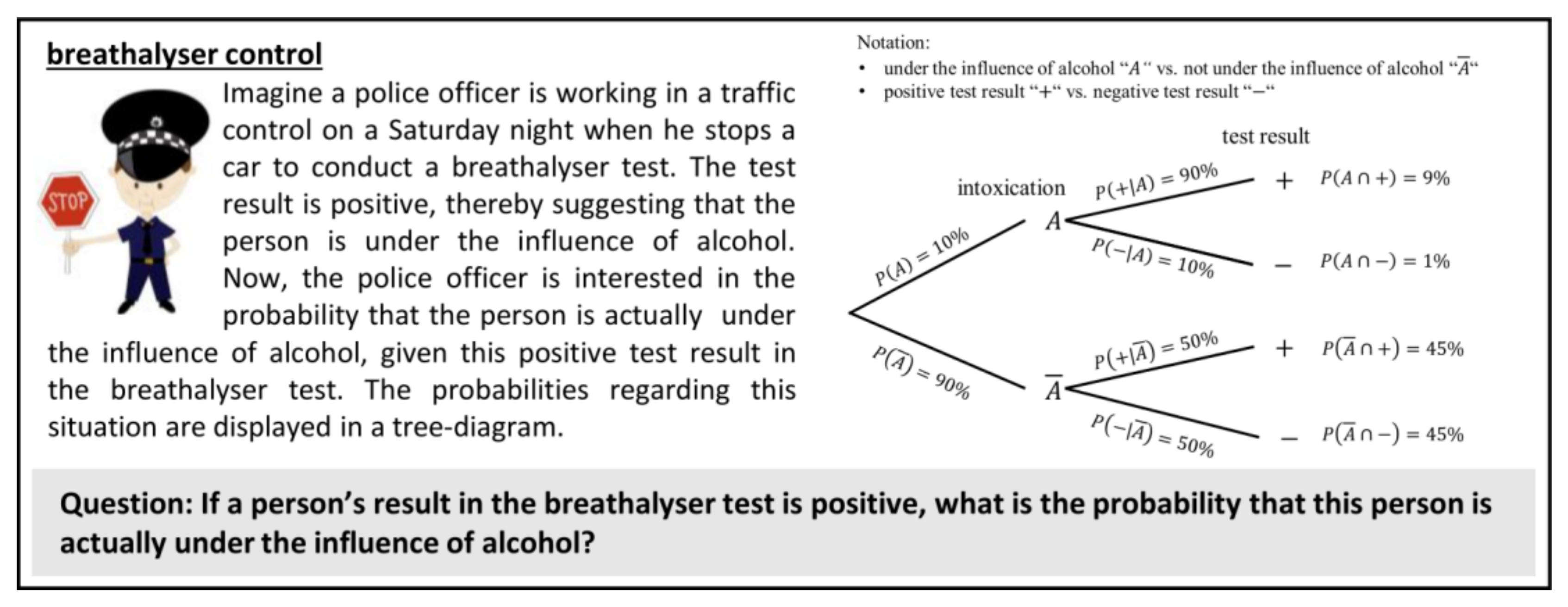
• The so-called base rate: the a priori probability that the hypothesis is true (prior to the presence of an indicator). In the example above, this corresponds to the probability of a person stopped by the police being under the influence of alcohol on a Saturday night, $P\left(A\right)$.
• The so-called true-positive rate: the probability that an indicator is present when the hypothesis is true. In the example above, this corresponds to the probability that the result of a person’s breathalyser test is positive, if that person is indeed under the influence of alcohol, $P(+|A)$.
• The so-called false-positive rate: the probability that an indicator is present even though the hypothesis is false. In the example above, this corresponds to the probability that the result of a person’s breathalyser test is positive even if that person is not under the influence of alcohol, $P(+|\overline{A})$.

Most often, Bayesian Reasoning is studied concerning the ability to calculate a conditional probability with these given parameters. Usually, one of the following two probabilities is to be determined in a Bayesian problem:

• The so-called positive predictive value (PPV): the probability that a hypothesis is actually true, if an indicator is given. In the example above, this corresponds to the probability that a person is actually under the influence of alcohol, if the breathalyser test is positive, $P(A|+)$.
• The so-called negative predictive value (NPV): the probability that a hypothesis is actually false, if no indicator is given or information is given which suggests that the hypothesis is false. In the example above, this corresponds to the probability that a person is actually not under the influence of alcohol, if the breathalyser test is negative, $P(\overline{A}|-)$.

With the probabilities given in the exercise in Figure 1, the application of Bayes’ formula results in $P\left(A|+\right)=\frac{0.1\times 0.9}{0.1\times 0.9+0.9\times 0.5}\approx 17\%$ for the PPV and $P\left(\overline{A}|-\right)=\frac{0.9\times 0.5}{0.9\times 0.5+0.1\times 0.1}\approx 98\%$ for the NPV.

A large variety of studies have contributed to the research on Bayesian Reasoning by studying the influence of different variables on the ability to calculate the PPV or NPV. However, calculating an outcome (e.g., in this case, the PPV) is only one facet of operating with the formula. Another desired facet of operating with a formula is described by Sokolowski [24]. He points out “it is believed that teaching students how to perceive formulas as covariational entities based on the provided context is essential. This skill can enable them to consider formulas as dynamic functions” [24] (p 184). Even though Sokolowski has emphasised the importance of “formulas as dynamic functions” for understanding physics, we consider it to be of equal importance in the Bayes’ formula with regard to understanding conditional probabilities. For example, Borovcnik [25] demands that opportunities should be created to “investigate the influence of variations of input parameters on the result“ (p. 21) in order to develop a conceptual understanding of conditional probabilities. Adopting the perspective of Bayes’ formula as a function (of three variables, which is rarely taken in empirical research) opens up the possibility of applying insights from research about the understanding of functions to Bayesian Reasoning as well. With Bayes’ formula at the root of Bayesian Reasoning, we propose to generalise the idea of using Bayes’ formula as a “dynamic function” by relating the different aspects of the concept of functional thinking to Bayesian Reasoning:

• Static aspect of Bayesian Reasoning: interpreting the formula’s structure in the sense that the given parameters (e.g., base rate, true- and false-positive rate) directly correspond to one result (e.g., PPV), which is calculated. This relates to the aspect of mapping in the concept of functional thinking [26,27] or the action conception of a function [28], because three given parameters, e.g., the base rate $P\left(A\right)$, the true-positive rate $P(+|A)$ and the false-positive rate $P(+|\overline{A})$, interpreted as independent variables, are used to calculate the requested dependent variable PPV $P(A|+)$. Thus, the solution $P(A|+)$ is a function value mapped to the three given variables $P\left(A\right)$, $P(+|A)$, and $P(+|\overline{A})$ via the Bayes’ formula. In Bayesian Reasoning, we refer to the ability to map three given parameters to the solution of Bayes’ formula as the aspect of performance (with or without the explicit use of Bayes’ formula).
• Dynamic aspect of Bayesian Reasoning: interpreting the formula’s structure in the sense that changes in the given parameters (e.g., base rate, true- or false-positive-rate) influence the result (e.g., the PPV). This relates to the aspect of covariation of the concept of functional thinking [26,27] or the process conception of a function [28] because a variation in one (or more) of the parameters being interpreted as independent variables (e.g., base rate $P\left(A\right)$, true-positive rate $P(+|A)$ or false-positive rate $P(+|\overline{A})$) alters the dependent variable (e.g., PPV $P(A|+)$) when $P\left(A|+\right)$ is understood as a function value of the Bayes’ formula, which is seen as a three-dimensional function with the given parameters (e.g., base rate, true- and false-positive rate) as the independent variables. Consequently, we refer to the ability to evaluate the influence of changes to the given parameters on the result of Bayes’ formula as the aspect of covariation.

Thus, the static and dynamic aspects (of Bayesian Reasoning and the concept of functional thinking) describe different ways of thinking (about Bayesian situations and functions) while performance and covariation relate to different abilities (in Bayesian Reasoning and working with functions). To the best of our knowledge, Bayesian Reasoning has (so far) been studied almost exclusively with regard to the static aspect by measuring performance. It has been shown that without any supportive strategies, performance in Bayesian Reasoning is generally very poor [6]. However, successful strategies have been identified to support performance in Bayesian Reasoning: The first one is the use of so-called natural frequencies, as the format of the given statistical information (see, e.g., [5,6,29,30,31,32,33]) improves the performance of Bayesian Reasoning. In this strategy, a pair of natural numbers is used to describe the probabilistic information and can represent an expected frequency in a fictitious sample [33]. The concept of natural frequencies was introduced by Gigerenzer and Hoffrage [33] and a comparison of the given information in form of probabilities and natural frequencies is given in

Table 1. Information provided in a Bayesian situation in form of probabilities and natural frequencies.

	Probabilities	Natural Frequencies
base rate	The probability is 10% that a person stopped by the police is under the influence of alcohol on a Saturday night.	10 out of 100 people are under the influence of alcohol when stopped by the police on a Saturday night.
true-positive rate	If a person who is under the influence of alcohol is tested, the probability is 90% that the breathalyser test is actually positive.	In 9 out of 10 people who are under the influence of alcohol, the breathalyser test is actually positive.
false-positive rate	If a person who is not under the influence of alcohol is tested, the probability is 50% that the breathalyser test is positive nevertheless.	In 45 out of 90 people who are not under the influence of alcohol, the breathalyser test is nevertheless positive.

. The second successful strategy is to use adequate visualisations as a representation of the Bayesian situation (see, for example, [7,15,34,35,36,37]). This strategy is explained in more detail in Section 2.2.

The dynamic aspect of Bayesian Reasoning, e.g., by measuring covariation, has only rarely been studied. Yet, Böcherer-Linder et al. [38] showed that the visualisation also affects covariation in Bayesian problems. Hence, (adequate) visualisations are a supportive tool for the static, as well as dynamic, aspect of Bayesian Reasoning. We propose that dynamic visualisations can be particularly supportive for tasks which address the dynamic aspect (dynamic tasks) while static visualisations are preferable for tasks which address the static aspect (static tasks) in Bayesian problems, in order to closely tie the specific demands of the task to its supportive strategy.

With this introduction on Bayesian Reasoning, we aim to highlight that specific Bayesian problems can differ with regard to the aspect of Bayesian Reasoning (static or dynamic) which is addressed by a specific task. Additionally, the support that is provided in the problem can be varied by using different strategies (i.e., natural frequencies and visualisations).

2.2. Visualisations and Bayesian Reasoning

An overview of typical visualisations for Bayesian situations can be found in Spiegelhalter et al. [7] or Binder et al. [29]. Furthermore, Khan et al. [15] have categorised these visualisations into three groups: (1) nested-style, (2) frequency-style, (3) branch-style. In Figure 2 (compare Section 1), an overview of some of the visualisations discussed here is given. They are presented without particularly supportive design-elements from a multimedia point of view (upper three rows). However, they already provide an idea of what visualisations may look like when designed according to multimedia principles (lowest row). Empirical studies have investigated a wide variety of visualisations that have been proven to support Bayesian Reasoning: tree diagrams (e.g., [13,29,39,40]), double-trees (e.g., [15,34,41]), unit squares (e.g., [42,43,44]); 2 × 2 tables (e.g., [35,45]), icon arrays (e.g., [36,46,47]), frequency nets [34,48] and others were all found to increase performance in Bayesian Reasoning. However, there are also visualisations that provide little or no support (e.g., Euler diagrams as in [49]). Moreover, comparisons between the helpful visualisations showed that some of these are more helpful than others. For example, tree diagrams help only when absolute frequencies are displayed within the diagram, rather than probabilities as in Figure 1 [29]. The double-tree and unit square are significantly more helpful than the common tree diagram (even if absolute frequencies are used in the tree diagram) [50]. Both the aforesaid visualisations (double-tree and unit square) are comparably helpful, with around 60% of participants revealed as able to solve a Bayesian problem when it is displayed in a double-tree or unit square with frequencies. Empirical results suggest that other visualisations such as a frequency 2 × 2 table and icon arrays may even outperform the double-tree and unit square regarding performance [34,50], yet we consider them less supportive for covariation (see below).

We wish to point out that, in this and the following analyses, we regard visualisations as a support for Bayesian problems in which the base rate, true- and false-positive rates in form of probabilities represent the given information, as this is the most common case in authentic situations. Moreover, we only refer to the statistical information given directly within the visualisations. In concrete tasks, there may be further information in the text surrounding the visualisation. However, we focus on the design of the visualisations here (for designing textual information according to multimedia principles, also see [8]).

As well as taking into account empirical results, subject-didactical and educational perspectives also need to be considered when selecting a particular visualisation as a supportive strategy in a Bayesian problem. For instance, some visualisations require time-consuming drawing and are therefore not very suitable in a context where the subsets change or the visualisation needs to be self-drawn, at least when large sample sizes are given (e.g., icon arrays). Therefore, we do not focus on icon arrays in this paper as a supporting visualisation. Additionally, an analysis of the demands of the Bayesian problem can help to identify characteristics of the visualisation that are necessary to solve the problem. Consequently, we will now evaluate (from a theoretical point of view): which relationships does a visualisation ideally display for (1) supporting the static aspect of Bayesian Reasoning (in static tasks), and (2) supporting the dynamic aspect of Bayesian Reasoning (in dynamic tasks)?

• Static tasks: Static tasks address the static aspect of Bayesian Reasoning. Therefore, in static tasks, the three given parameters are used to calculate the PPV (for example with Bayes’ formula). Bayes’ formula for two dichotomous events can be simplified to two conceptually simpler ratios: $P\left(A|+\right)=\frac{P\left(A\right)\cdot P(+|A)}{P\left(A\right)\cdot P(+|A)+P\left(\overline{A}\right)\cdot P(+|\overline{A})}=\frac{P\left(A\cap +\right)}{P\left(A\cap +\right)+P\left(\overline{A}\cap +\right)}=\frac{P\left(A\cap +\right)}{P\left(+\right)}$.
  Both transformations have a simpler structure than the original Bayes’ formula. As a consequence, we argue that a visualisation that represents the equivalence of these algebraic transformations can more easily lead to simpler (and correct) calculation of the result (even if the formula is not explicitly used in the teaching process). In order to do so, two equivalences should be observable in the visualisation: first, the equivalence of the product of the simple and conditional probability to the joint probability (first equal sign), and second, the equivalence of the sum of the two intersects (the true- and false-positives) to their shared superset (all positives; second equal sign). Consequently, in order to be supportive for static tasks, we argue (from a subject-didactical perspective) that it is important that the visualisation (in addition to the three pieces of information given in the task itself) shows these two intersections (or associated joint probabilities), and also makes it transparent that they both belong to the same superset. In doing so, the solution to static tasks of Bayesian Reasoning should become easier from a theoretical point of view.
• Dynamic tasks: Dynamic tasks address the dynamic aspect of Bayesian Reasoning. The question here is how modifications in the given parameters affect the result (PPV, NPV). Therefore, from a subject-didactical perspective, we regard it as important that the three pieces of information, which are given in the task itself, can be represented at all, and that the structure of the visualisation can visually represent how a change in these parameters affects the result (or the relevant intersections/joint probabilities).

The aspects relevant to static and dynamic tasks are implemented differently in the various visualisations (

Table 2. Different realisations of the aspects relevant for static and dynamic tasks in simple tree diagrams, double-trees, 2 × 2 tables and unit squares.

	Tree Diagram	Double-Tree	2 × 2 Table	Unit Square
Static tasks
Given probabilities	Represented on the branches	Represented on the branches	Not directly represented	Represented as the ratio of the division of the sides
Representation of the two relevant intersections (joint probabilities)	Joint probabilities can stand at the end of one path (probability tree) or intersections as frequencies in the nodes at the end of one path (frequency tree)	Intersections given in in the nodes of the middle level as frequencies	Intersections given in the inner fields as frequencies (2 × 2 table with frequencies) or joint probabilities given as probabilities (2 × 2 table with probabilities)	Intersections given as frequencies inside the inner areas and as the size of the inner areas
Belonging of the intersection (joint probability) to the superset	Expressed through the connection of the intersection to the superset by a branch; only given for one superset (node above the intersection)	Expressed through the connection of the intersection to the superset by a branch; given for both supersets (node above and below intersections)	Expressed through the adjoining positions of the inner fields: next to each other (as a row) or underneath each other (as a column)	Expressed through the adjoining positions of the areas (as in the 2 × 2 table)
Dynamic tasks
Dependence of the intersection (joint probability) on the given information	Connectedness of the nodes with the branches reveals the influence of the parameters on the associated absolute frequencies	Connectedness of the nodes with the branches reveals the influence of the parameters on the associated absolute frequencies	Cannot be visualised, as given probabilities are not directly represented	Size of the inner areas (i.e., intersections) depends on its length and width, which correspond to the ratios of the divisions on the sides (i.e., the given probabilities)

).

In Table 2 we provide two pairs of related visualisations, which differ regarding their support for the static and dynamic aspects: the double-tree is a progression of the simple tree diagram and the unit square can be seen as a 2 × 2 table with additional geometric features of area-proportionality [51] (please also see Figure 2 for an overview of the relevant visualisations). All four visualisations can represent the two relevant intersections. Additionally, the pairs of visualisations share certain characteristics. Both types of tree-diagrams (simple tree diagrams and double-trees) express membership of the superset through a connection by a branch. In contrast, in the unit square and the 2 × 2 table, belonging to the superset is expressed through the adjoining positions of the inner fields. Apart from that, both the unit square and double-tree represent aspects that cannot be represented in their related visualisation: The double-tree can represent membership of both supersets (which is not possible in the simple tree diagram) and the area-proportionality of the unit squares can represent given (conditional) probabilities and also their influence on the intersections (which is not possible in the 2 × 2 table). Thus, regarding the theoretical analysis of requirements of a visualisation for a Bayesian problem from a subject-didactical point of view, the nature of 2 × 2 tables seems problematic for dynamic tasks especially, since the true- and false-positive rates (typically given in a Bayesian problem) cannot be visualised directly. Hence, even though empirical results have shown that 2 × 2 tables are a supportive visualisation for static tasks of Bayesian Reasoning, we argue against them for dynamic tasks especially. However, two visualisations that have been identified as supportive for static tasks from an empirical perspective also stand out for their favourable characteristics in theoretical analysis: the double-tree and unit square. They both represent the relevant subsets, which are necessary for static tasks of Bayesian Reasoning, and also display the dependence of the intersections or joint probabilities on the given parameters. Therefore, they are (unlike the other visualisations discussed) suitable for Bayesian Reasoning from both empirical and theoretical perspectives. Therefore, in the following sections of this paper, we focus on describing how to design these two options.

2.3. Aspects of Multimedia Learning

Working with multiple representations (such as the textual description of a Bayesian problem together with a visualisation of the Bayesian situation) can serve different functions. Ainsworth [52] distinguishes three essential functions. Firstly, multiple representations can complement each other (complementary function). Secondly, the multiple linkage of representations is also suitable for explaining a little-known, or completely unknown, representation with a more accessible representation (constraining function). Finally, multiple representations can support the construction of deeper understanding (constructing function) by revealing underlying structures of a content concept through their different forms of presentation and the way they are linked. These functions are not mutually exclusive, but one set of representations can fulfil multiple functions [53]. All in all, multiple representations can support the process of extraction and transferral that takes place when learners recognise that a concept represented in a certain way can also be represented in another way, and learn how to do so on their own. Arguments for this beneficial effect of using multiple representations can be found in theories of multimedia learning.

2.3.1. Processing Multimedia Material

According to Schnotz [54] (p. 72), the term ‘multimedia’ at the level of presentation format refers to “the use of different forms of representation such as text and pictures”. Text can be in printed or spoken format and the pictures include static pictures (photos, figures, diagrams, …) and/or dynamic pictures (videos, animations). Therefore, solving a Bayesian problem with the help of a visualisation implies the use of multimedia.

Two theories of multimedia learning are at the forefront of research: Mayer’s [55] Cognitive Theory of Multimedia Learning (CTML), and the Integrated Model of Text and Picture Comprehension (ITPC) of Schnotz [54]. Both of these theories propose arguments as to why using multimedia fosters learning, a consequence which is also known as the multimedia-effect (a “benchmark finding” according to Schweppe et al. [56] (p. 24)) and which may occur when solving a Bayesian problem, for example.

According to Mayer’s [55] CTML, working memory has two channels in which externally represented information can be processed via mental representations: one channel for (printed or spoken) verbal information and one for non-verbal information. The capacity of these channels is limited but their independence from each other means that they are not competing to achieve greater capacity [55]. Separate mental representations of two channels are integrated into a coherent mental model when appropriate prior knowledge is retrieved from long-term memory. If, for example, a non-verbal graphical representation of given textual representation is generated, this means that two, instead of one, channels are involved. As cognitive capacity is limited, using both channels means that more working memory resources are available and can be used to, e.g., deepen understanding.

By problematising the assumption of parallel text and image processing of Mayer’s CTML [55] within a theoretical point of view the ITPC model of Schnotz [54] points out the fundamental assumption that texts and images are based on different sign systems and therefore follow different principles of representation. However, from a practical point of view, the ITPC model [54] is consistent with the CTML regarding its outcomes for designing multimedia-based learning environments.

This means that, according to CTML as well as ITPC, it can be theoretically reasoned that the use of double-trees or unit squares (which complement the text of a Bayesian problem) results in more available and sophisticated mental models compared with use of the text of the Bayesian situation alone. However, it is important to recognise that combinations of representations, such as the description and depiction of a Bayesian situation, are not helpful per se, but processing multiple external representations (MERs) can evoke translation processes between single representations which may be difficult and cognitively demanding. Thus, such translation processes should be carefully planned, designed and implemented in the learning setting, i.e., the Bayesian problem.

2.3.2. Cognitive Load

One theoretical reference theory for planning and designing learning scenarios, (particularly regarding cognitive demand), by using MERs is Sweller’s Cognitive Load theory (CLT; [57]). This theory integrates knowledge about limited working memory capacity with design principles for instructions, to reduce unnecessary cognitive load in order to enhance learning. It is often used in combination with Mayer’s [55] CTML. According to CLT, the cognitive load imposed on working memory originates from three categories of cognitive load [57]: intrinsic cognitive load (ICL), extraneous cognitive load (ECL) and germane cognitive load (GCL). The ICL of a subject matter derives from its complexity and the learner’s prior knowledge. The ECL refers to the cognitive load of aspects that are irrelevant to learning. This depends in particular on how the external representation of learning materials is designed. GCL refers to the cognitive load relevant to learning; in this approach, it is a desirable type of load. However, according to latest research, GCL is no longer assumed to contribute to the total cognitive load by assuming that GCL “has a redistributive function from extraneous to intrinsic aspects of the task rather than imposing a load in its own right” [58] (p. 264).

For our purposes, this means that: if either ICL and/or ECL in the Bayesian situation is high, working memory can become overloaded and inhibit successful learning [59]. Unlike ICL, which is inherent to the Bayesian problem itself, ECL can be reduced by changing the design of instructions [58]. Thus, the cognitive processing of any surface features (such as the visualisation which depicts the Bayesian situation) that are non-essential to the content can be reduced.

2.3.3. Design Principles

There are several design principles and guidelines for the design of educational material which different researchers derive from theories of multimedia learning (e.g., CTML) on the one hand and from CLT on the other hand with the goal of supporting multimedia learning and reducing ECL.

In this paper, we do not report all the principles of multimedia learning and design guidelines to optimise cognitive load (for an overview see [55,60]), but we refer to those features which are of special interest from a theoretical viewpoint regarding the design of visualisations, such as the unit square and double-tree used in Bayesian problem situations.

Split-attention: When learners are required to split their attention between at least two sources of information (e.g., text and diagram), one is speaking of a split-attention effect [61]. Split-attention can be caused by either spatial or temporal separation and increases ECL, which might inhibit learning (e.g., [62]). Research results suggest that a split-attention design has negative consequences and should be replaced by an integrated-format design, where relevant data are presented close to each other [63]. This could be an additional argument (alongside the empirical and theoretical reasonings from Section 2.2) against tree diagrams, as the two intersecting paths that belong together are not close to each other and therefore hard to recognise as belonging together, since the observer’s attention is split. Thus, in Section 3, we present design realisations of the double-tree and unit square, where the relevant information is not, or as little as possible, spatially separated.

Redundance: The redundancy effect (similar to Mayer’s redundancy principle [12]) suggests that learning is hindered when learners are presented with the same information in two or more forms, and/or with additional information that is not relevant for solving the task [64]. Processing redundant information takes up working memory capacity that could be put to better use. Research shows that eliminating redundant information from tasks results in enhanced learning (e.g., [65]). Consequently, we pay attention to designing the visualisations in Section 3 in such a way that each information is presented in one form only.

Coherence: Similarly to the redundancy principle, the coherence principle states that people learn better when extraneous material is excluded rather than included [12]. This means that words, audio and graphics that do not support instructional goals should be removed since they cause irrelevant cognitive load as learners’ working memory is overloaded with distracting details that do not contribute to the learning goals. The aim is to support coherence formation [66] between different multiple representations, since knowledge acquisition requires creating referential connections between corresponding representational elements in different formats. The coherence principle may be particularly important for learners with low working-memory capacity or low domain knowledge [67]. Therefore, in the realisations of the double-tree and unit square in Section 3, we specifically emphasise aspects of the visualisations concerning design features which support the goal of the learning scenario (e.g., the identification of the relevant subsets for calculating the PPV) but are mindful not to insert additional design features for irrelevant aspects of the Bayesian problem.

Signalling: According to van Gog [68], the signalling principle refers to the finding that people learn better with multimedia when supported by attention-guiding cues to the relevant elements of the learning material (e.g., via highlighting). Research reports on three different kinds of cues: picture-based cues (e.g., [69,70]), text-based cues (e.g., [71,72]) and cueing of corresponding elements in written text and pictures (e.g., [73,74]). Throughout research on signalling, colour coding is important because it is a frequently used element in all three different kinds of cueing mentioned previously. Although there were mixed findings regarding significance and effect sizes in studies of different kinds of cueing, it can generally be stated that most studies reveal cueing to have a positive effect on cognitive load and learning outcomes (cf. [68]). As a result, we use the signalling principle as a means to design the double-tree and unit square in Section 3 by highlighting particularly relevant elements of the visualisation for solving Bayesian problems.

Summing up Section 2, it becomes apparent that Bayesian Reasoning, where the Bayesian situation is characterised by text as well as visualisations, refers immediately to learning with multimedia material including symbolic representations (e.g., Bayes formula and its verbalisation) as well as different graphical representations, i.e., visualisations such as double-trees and unit squares on which we focus because they appear to be particularly advantageous.

3. Designing the Double-Tree and Unit Square

In this section we outline how we have integrated the above-mentioned implications from research on multimedia learning into digital realisations of the double-tree and unit square, which are used to support work on Bayesian problems. Thereby, we differentiate between static and dynamic realisations.

3.1. Static Visualisations

Static visualisations are used for Bayesian problems in which the static aspect of Bayesian Reasoning is addressed. There are many authentic scenarios in which the static aspect of Bayesian Reasoning is necessary, e.g., in the scenario when the police first stop a motorist. Unfortunately, probabilistic information (such as the characteristics of a breathalyser test or other diagnostic instruments) in the “real world” is most often given in probabilities and not in the more easily comprehensible frequencies. Thus, we adapt the visualisations so that both formats of statistical information are presented. According to Ainsworth [52], this could be regarded as the complementary function of visualisations. Therefore, the given probabilities (base-rate, true- and false-positive rate) as well as the complementary information in frequencies are displayed in the visualisation (Figure 3).

A Bayesian situation is usually characterised by two attributes (e.g., 1. intoxication of the person, 2. result in the breathalyser test) with two outcomes each (e.g., 1a. under the influence of alcohol, 1b. not under the influence of alcohol, 2a. positive test result, 2b. negative test result). Their combination results in four subsets (e.g., i. under the influence of alcohol and positive test result, ii. under the influence of alcohol and negative test result, etc.). These subsets are visualised in the double-tree as the four nodes in the middle level, and in the unit square as the four inner areas. Their relations to each other are expressed by the connectedness to different supersets, via the branches in the double-tree, and by being nested into to geometrically different superordinate structures (e.g., different rows and columns) in the unit square.

Generally, there are various ways to illustrate this 2-attributes × 2-outcomes structure in a multimedia context. In designing the double-tree and the unit square, we focused on the use of colours in the visualisations to highlight this structure by using different colours, different methods of colouring (colouring the surface vs. the border of a node, using different transparencies of the same colour, etc.) and different styles of the borders (colours or dashed vs. solid lines). In the following sections, the resulting different multimedia realisations are presented and directly evaluated with the principles of multimedia learning outlined above.

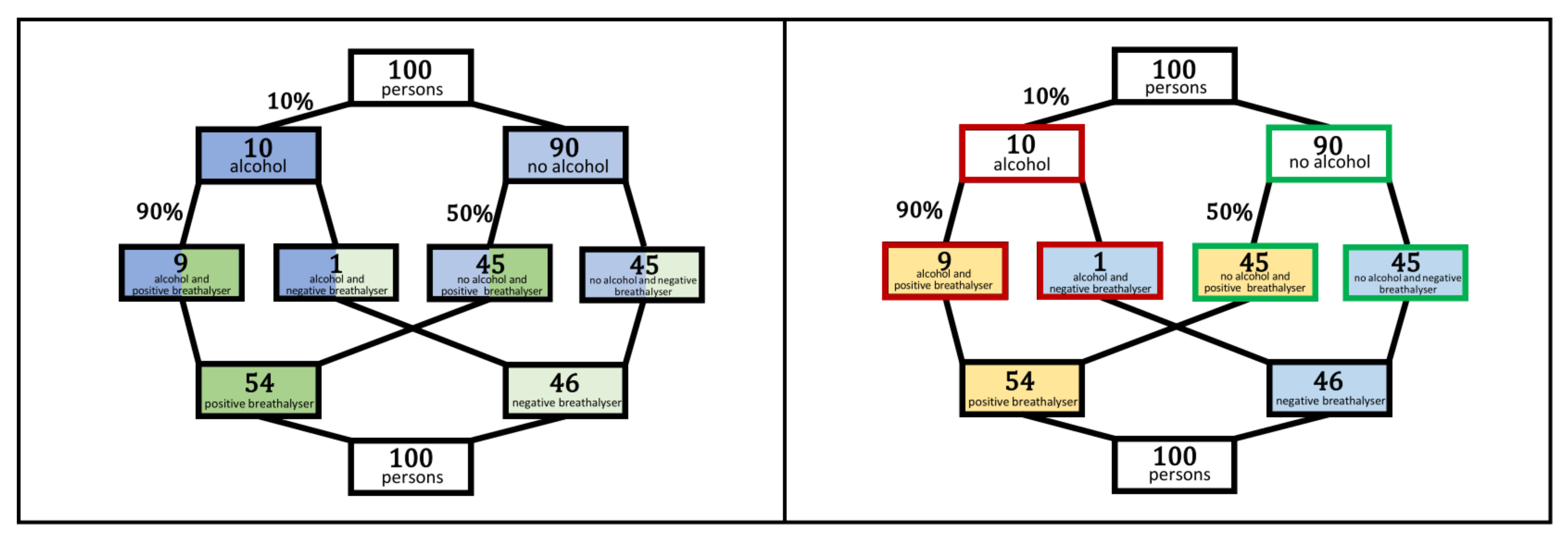
3.1.1. Static Double-Trees

The double-tree represents a node-branch structure that can be seen as an extension of the simple tree diagram. A major advantage of node-branch structures is that there is a fixed place for the frequencies (in the nodes) and a fixed place for the probabilities (on the branches). Through this structure, the helpful strategy of frequencies can be used to better understand the probabilities. In the double-tree (unlike the simple tree diagram), there are also nodes for the outcomes of the second attribute (e.g., positive vs. negative result in the breathalyser test) see Figure 2.

First, we considered whether the labelling in the double-tree should take place inside or outside of a node (see Figure 4).

Due to the split-attention principle, it makes sense from a multimedia point of view to position the text, i.e., the label, inside the representative node (double-tree on the right-hand side in Figure 4). Thus, the respective node is better linked with the label (i.e., the respective outcomes). Since the space in the node is limited, abbreviations must be used in some cases.

One difficulty of the double-tree is that two branches cross each other in the lower half. Thus, the number of individuals with positive tests is not composed by the frequencies directly above the node “positive breathalyser”. Consequently, in a second step, we set out to counteract the difficulty of crossing branches in the lower half by using different methods of highlighting according to the signalling principle (e.g., colouring the nodes). There are several different possibilities for highlighting, including the use of different colouring in the nodes or colouring the borders of the nodes. In addition, it would be conceivable to vary the type of lines linking the nodes.

Figure 5 shows two double-trees in which only colouring of the nodes according to the highlighting principle is used to clarify their belonging to different supersets.

In both cases, one colour is used for each outcome of an attribute. In this colouring method, however, the use of four different colours means that it is not possible to recognise which two outcomes belong to the same attribute. Thus, neither signalling method in Figure 5 is ideally suited for labelling the two attributes with two outcomes each. This disadvantage can be eliminated by working with one basic colour for each attribute and marking the outcomes of one attribute by a lighter or darker colouring (Figure 6, left). However, in those double-trees with two colours in one node (Figure 6, left; Figure 5), the impression could be conveyed that the number of people is always distributed in the same proportion. For example: half of the individuals under the influence of alcohol produce a positive breathalyser test and the other half of individuals under the influence of alcohol produce a negative breathalyser test. This impression is created by the equal proportions of the coloured areas in the middle level. Since the proportions of colourings of the inner nodes (50:50) do not correspond to the proportions of individuals with the respective outcomes of the attributes (as is the case with the unit square), this could represent a cognitive hurdle, which is why this signalling method would not appear to be optimal. Additionally, the redundancy principle suggests that this colouring method is not supportive, because two forms (two colours plus split area) are used to represent the intersections and therefore may elicit wrong interpretations. Thus, this form of misleading representation (a split area) is unnecessary and should be avoided. To avoid such misinterpretation, another method besides colouring only the inner part of the nodes must be used for highlighting, such as colouring the borders of the nodes (compare Figure 6, right).

The two different colouring methods (colouring the borders of the nodes vs. colouring the inner part of the nodes) highlight the two attributes differently. In the selected realisation (Figure 6, right) the result of the breathalyser test (positive vs. negative) is marked by the colouring of the inner part of a node, while the intoxication of a person (alcohol vs. no alcohol) is highlighted by colouring the border of a node. Reverse colouring methods would also be possible, i.e., a person’s intoxication is illustrated by colouring the inside of the node and the result of the breathalyser test is illustrated by colouring the border of the node. However, we chose the first option (Figure 6, right) because the upper part of the double-tree is analogous to the simple tree diagram and thus does not need to be emphasised to any particular degree. Furthermore, studies have shown that the crossed branches in the lower half make it difficult to correctly assign probabilities to the branches [34]. Thus, by colouring the inner parts of the nodes in the lower half of the double-tree it should be clear which two nodes belong to the node “positive breathalyser result” (or “negative breathalyser result”).

Furthermore, variations of the line types (rather than colouring of the border of the nodes) would have been conceivable. However, we decided against this highlighting method as it could cause confusion with regard to the lines from the branches. Presumably, one would then need several different types of lines to be able to differentiate clearly and this would unnecessarily increase the cognitive load.

3.1.2. Static Unit Squares

The unit square is related to the 2 × 2 table, as the same additional structure of the rows and columns is inherent in the unit square. An advantage of the unit square is that this structure is geometrically expressed by the area-representation. Thus, the areas of neighbouring inner fields always add up to the value of one row or column. The columns are just as easy to identify in the unit square as in the well-known 2 × 2 table. However, the rows are harder to recognise in the unit square since the horizontal division is usually (in the case of the two attributes not being stochastically independent) not on the same level for the neighbouring areas which add up to the value of one row. Consequently, there is no single division line which separates the upper from the lower row. In research on Bayesian Reasoning with unit squares, identifying the row has also been empirically identified as a difficulty of unit squares [35]. Therefore, we have used different design methods, which are specifically used to overcome this difficulty.

First, we altered the position of the labels in the unit square in order to more clearly illustrate the “rows” in the unit square. Thus, we aligned the labels on the left- and right-hand side of the unit square so that they are both on the same level as their counterparts and not displaced to a mid-height position adjacent to the area to which they correspond (compare Figure 7).

The split-attention principle suggests that recognition of the row should be easier in the second version of the unit square, as the left and right labels are now at the same height and therefore easier to identify as belonging to the same row.

Another way to highlight the rows in the unit square is to colour the areas of one row in the same colour and thereby make use of the highlighting principle. Two examples with different colours are displayed in Figure 8.

After colouring the rows it makes sense (a) to colour the labelling of the corresponding row (on the left- and right hand side) in the same colour as the areas which belong to this row (Figure 8) and (b) to use colours which are also clearly visible (such as green and blue, cf. [75]). Consequently, the colouring system with green and blue seems more appropriate.

The colouring method used so far only highlights the belonging of the inner area to the row. Thus, it neglects any membership of the inner area to the column. While the intention was to focus on the relation of the inner areas to the row, it might nevertheless be beneficial to use unobtrusive methods for signalling belonging to the column, in order to make the structure clearer.

In the first realisation (Figure 9, left), a line style was used in order to differentiate between the left and right columns. In the second realisation (Figure 9, right), the colour shade was varied to differentiate between the left and right columns. Both methods are less noticeable than the colouring of the areas itself (used to express their belonging to the row). As such, they correspond to the redundancy principle, since information which is already easy to identify (belonging to the column) is not reinforced in a second ostentatious way.

Finally, the frequencies in the unit square are so far only given for the intersections, not for the supersets. Even though the supersets are geometrically represented in the unit square (as the sum of both inner areas, which belong to the superset), it might be beneficial to also explicitly add this relation by adding the sums of the rows and columns (compare Section 2.2). However, according to the split-attention principle, it is important to also add the numbers in the vicinity of what they represent. We have considered two different ways of doing so (compare Figure 10).

While in the left realisation, the frequency is closer to the label of the attribute (the text), in the right realisation the frequency is closer to the geometrical feature of that attribute (the row or column). Depending on the context in which the visualisation is used, either one of these realisations can be more useful. In accordance with the split-attention principle, we propose focusing on the second realisation, if the geometrical aspects of the unit square are necessary or highlighted. Additionally, the left realisation seems unfavourable, as two numbers (frequencies and percentages) are right on top of each other. Furthermore, as the added frequencies represent sums (of the inner areas), the positioning in the right realisation is more natural in so far as sums usually appear in the lowest line (e.g., of addition by hand), or on the right-hand side of the equation. Finally, the positioning in the right-hand realisation makes the relation of the unit square to the 2 × 2 table more evident.

To summarise, in Section 3.1 we have shown that different design techniques can be used in order to emphasise the related nature of the different (sub-)sets of the structure of the Bayesian situation. Some of these techniques (e.g., colouring areas) are more eye-catching than others (e.g., line styles of borders, transparency of colours). Thus, they should be implemented carefully in order to facilitate recognition of more difficult relations (with use of more obtrusive methods) and easily understandable relations (with use of less ostentatious methods).

We have analysed the difficulties in the double-tree and the unit square in order to implement these different methods effectively. In doing so, we hope to have presented a design of each of the visualisations which clarifies the relations in the structure of the Bayesian situation. Consequently, this design should support identification of the relevant subsets which are needed in order to calculate a required probability (e.g., PPV or NPV). In the next section, we will discuss design possibilities for dynamic realisations of the same visualisations.

3.2. Dynamic Visualisations

The dynamic visualisations are relevant for assessing the influence of changes in the given parameters on the PPV. As the PPV is calculated with the ratio comprising the two relevant subsets (e.g., true-positives and false-positives), it is necessary firstly to assess the influences of changes in the given information on these subsets and, secondly, to identify the consequences of these changes for the ratio.

Thus, assessing changes in a Bayesian situation is fairly complex as, for instance, changes in the base rate affect all four subsets simultaneously. As a consequence, the ICL when evaluating the change of the base rate (for example) is assumed to be fairly high. A dynamic visualisation where the changes within the structure are observable through the employment of a slider can help to identify those changes [76,77]. Yet, as it is a demanding task where multiple changes are observable and ICL is high, it needs to be very carefully designed in order to minimise ECL.

3.2.1. Dynamic Double-Tree

In the double-tree, the probabilities given in a typical Bayesian task are found as percentages on the branches in the upper half of the visualisation (e.g., Figure 11). Various positions are conceivable for the arrangement of a slider with which the three percentages can be changed. Basically, two different positions can be discussed: (1) A slider along a branch (2) A horizontal slider (on a node). We argue that these different positions of the slider may represent different conceptual ideas about percentages and, therefore, also probabilities. Thus, we rely on two fundamental mental representations about fractions (here: realised as percentages) [78]: (i) fraction (or percentage) as a part–whole relationship and (ii) fraction (i.e., percentage) as the idea of odds. Then, by applying these conceptual ideas to the interpretation of probability, the first idea of a part–whole relationship leads to the understanding that a probability represents a smaller part of a reference group (i.e., the whole). In that case, the given percentage for a probability (e.g., 10% for the base rate) specifies the proportion of the whole (i.e., all the people who are tested) for whom the attribute of the probability (i.e., being under the influence of alcohol) applies, i.e., 10% of all people are under the influence of alcohol. On the other hand, the second conceptual idea of odds leads to the understanding that a probability specifies the chances for both outcomes of a particular attribute by way of a ratio of the two subsets simultaneously. Then, the given percentage (e.g., 10% for the base rate) stands for a ratio of 10% to 90% by which the chances for the different outcomes (i.e., the state of being or not being under the influence of alcohol) are assigned. The two proposed positionings aim at deploying these two different ideas of probabilities, i.e., the part–whole relationship and the idea of odds (see Figure 11).

The slider along a branch: The branch in the double-tree connects the part with the whole. Thus, positioning the slider on the branch, results in an emphasis of the part–whole relationship. Moreover, colouring the percentage of the branch which corresponds to the probability on the branch also highlights this feature. Therefore, increasing the percentage on the branch with a movement of the slider directly illustrates that more of the whole (i.e., the node at the upper end of the branch) now belongs to the part (i.e., the node in the lower end of the branch). However, in the double-trees, there are always two branches that stem from one node, which means that with one probability $P\left(A\right),$ also its complement $P\left(\overline{A}\right)$—despite not being depicted as a percentage—is visualised (i.e., on the adjacent branch). Therefore, a second slider must be arranged at the adjacent branch, which represents the complement. This second slider then moves automatically when the first slider is changed. This might result in the learning effect that you can observe: a probability and its complement always change inversely to each other and always add up to 100%. Yet, this is a relatively basic concept which we consider rather simple, so this simultaneous move could be eliminated here. Moreover, this representation has major disadvantages from a multimedia point of view: many changes occur simultaneously (as well as all numbers, which need to change, also two sliders move at the same time) and, moreover, one slider moves automatically which is counter-intuitive as usually the concept of a slider is that it only changes if you drag its handle. Therefore, this realisation increases cognitive load and diverts attention away from the essential concept, namely the change in the relevant frequencies for the PPV.

The horizontal slider (on a node): On the other hand, the positioning of the horizontal slider (on a node) relates to the idea of odds (e.g., 10:90). The considered quantity (in the upper node) is divided into two disjoint outcomes by only one slider, and thus a change of one percentage number. The ratio of the given probability is immediately observable on the slider itself, which shows clearly (compared to the slider along a branch) that the sum of the probabilities of event and counter-event is 1. Thus, it also illustrates how the sample in the Bayesian situation (i.e., all people tested) is divided into the different subsets (by the respective ratio). Furthermore, with this positioning—in contrast to Figure 11, left—only one slider per pair of branches is necessary. Thus, cognitive resources can be saved and applied to the observation of changes in the relevant frequencies.

With this type of slider, we believe there are two possible different arrangements. One, where the slider is between the two branches of the respective probability (Figure 11, middle) and another, where the slider is attached directly to the nodes (Figure 11, right).

In the illustration (Figure 11, middle) where the horizontal slider is positioned between the two branches, an additional line is required for the slider. This may cause confusion because each branch (which is marked by a line) stands for a concrete probability. However, due to the node-branch structure in the double-tree, the horizontal lines in the node itself can be used (in order to avoid confusion, Figure 11, right). Therefore, in the realisation on the right of Figure 11, the bottom horizontal line of a node is used to place the slider directly on this border of the node. Then, it is also clearly evident that the population (from the node) is divided into the two following subsets (given in the nodes beneath) by the ratio of the slider. Thus, we prefer the double-tree on the right-hand side of Figure 11 as a positioning of the slider.

In addition to the positioning of the sliders, it is also useful to highlight the sliders and the associated percentage on the respective branch by colouring. This makes it easier to see which percentage can be changed by the slider (compare Figure 12, left). Since changing one of the three probabilities (such as the base rate) in the double-tree can change up to eight frequencies (all except the number of the sample) at the same time, it makes sense to also focus attention on the frequencies that are relevant to the task at hand (coherence principle). For example, if the effect of change of the true positive rate on the PPV is concerned, it makes sense to highlight only the changing probability and the relevant frequencies in the visualisation (compare Figure 12, right).

3.2.2. Dynamic Unit Square

Similar matters need to be given consideration in the design of dynamic unit squares. Here, changes in the given parameters result in different positions of the dividing lines in the unit square. Thus, due to the area representation of the unit square, changes to the Bayesian situation are linked to changes in size of the inner areas in the visualisation (compare Figure 13).

This feature makes the positioning of the slider more straightforward than in the double-tree, as the sliders should be clearly associated with the dividing line (which is “moved” by a change to its value). Thus, the use of a slider makes this change even more dynamically “observable”.

There are basically three possible locations for the slider: (1) next to the dividing lines, (2) inside the unit square on the line they are moving, (3) on the side of the unit square (see Figure 14).

According to the split-attention principle, the slider should be spatially as close to the changing object as possible. Consequently, we prefer the second and third realisation of the slider as the sliders in these versions are closer to the dividing line they move. In the second realisation, the handle of the slider is further away from the percentage it changes than in the third. Moreover, sometimes (as in the example in Figure 14 in the middle) the position of the handle on the vertical line is unfortunate, as it is at the same height as one (or both) of the horizontal lines and thus it might be unclear what the slider is actually changing. Finally, the most crucial change is to the division on the sides (with changes of the given parameters), as the movement of the inner dividing lines are only a consequence of the changes in ratios on the side of the square. Therefore, our preferred version is the third realisation, where the handle of the slider is closest to the relevant changing feature.

As well as positioning the slider, its colour can be used to facilitate recognition of its connection to the percentage and line segment, which the slider changes (as already spelled out in the double-tree). We need to bear in mind that the slider changes three aspects simultaneously: (i) the percentage, (ii) the line segment on the side of the unit square, (iii) the position of the corresponding dividing line inside the unit square. By colouring the slider in a specific way, the reference to some, or all, of these aspects can be spelled out (see Figure 15).

In the colouring of the first two realisations, only two of the features which change are highlighted. However, the third realisation highlights the relation to all relevant features that are linked to, and changed, by the slider. Therefore, we argue that this is the easiest dynamic realisation of the unit square, where it is clearly evident which properties of the visualisation are affected by a change in the percentage.

Finally, we now discuss whether the frequencies in the unit square can or should be removed in a dynamic version of the unit square. The redundancy principle suggests that learning is hindered if information is presented in two or more forms. The four subsets in the unit square are represented by the size of the inner area as well as the frequency, which is inside that area. While the frequency is crucial in being able to determine the PPV (hence the static aspect is addressed), it is not necessary to be aware of concrete numerical changes in order to assess the influences of changes to a given percentage (when the dynamic aspect is addressed). Therefore, we argue that frequencies are redundant for the dynamic setting, and should be removed from the visualisation.

Removing the frequencies from the unit square has another advantage. If the percentages are close to 0% or 100%, one or multiple inner areas become so small that the number of the frequency no longer fits into the inner area. This would result in an ambiguity about what the number actually represents (see Figure 16, left). This problem is avoided by removing the frequencies but not the percentages (see Figure 16, right). This is particularly important for the dynamic visualisation since, in the dynamic aspect, the focus is not on concrete numbers (unlike in the static aspect, where the concrete numbers are indeed relevant and should not be removed).

4. Discussion

We have presented an approach for designing visualisations, which is based on the following elements. Firstly, it is necessary to analyse the specific demands of the mathematical tasks. We showed this in Section 2.1 through a discussion of the different aspects of Bayesian Reasoning, which demand different types of visualisations: tasks addressing the static aspect of Bayesian Reasoning should be supported with a static visualisation, whereas tasks addressing the dynamic aspect of Bayesian Reasoning should be supported with a dynamic visualisation. Secondly, it is necessary to select a visualisation type. We argue that two types of considerations should be involved in this decision: previous empirical results and subject-didactical considerations. In Section 2.2, we have first provided empirical results of comparisons between different visualisations for Bayesian problems. Afterwards, we have discussed probability tree diagrams, double-trees, 2 × 2 tables and unit squares from a subject-didactical perspective, by comparing how different subsets and their relations to each other are represented in the different visualisations. Through the combination of both considerations, we opted for the double-tree and the unit square [50]. The third element of our approach is the actual design process of the visualisations. For that, we used principles of multimedia learning [55,60], which were presented in Section 2.3 [79], and applied them to the design of the visualisations in Section 3. In the design process, the multimedia principles are used primarily for two goals. First, they are used for reducing difficult aspects of the visualisations, which have previously been identified (e.g., identifying the “rows” in the unit square, which was a recommended finding from previous empirical studies). Second, the multimedia principles are used to highlight the task-specific aspects within the visualisation (e.g., the sliders are coloured in the same colour as the number they alter). Finally, subject-didactical considerations are also relevant in the design process, e.g., for positioning the sliders in the double-tree. We have presented the different decisions relevant within the design-process in a step-by-step development of the double-tree and unit square. In doing so, we discussed the advantages and disadvantages of every option arising in the decision-making process.

In the following passages we demonstrate briefly how this approach can be applied to other visualisations that can be used to represent a Bayesian situation, and thereby broaden and generalise the results presented in Section 3.

As mentioned at the beginning, probability tree diagrams as representations of Bayesian situations are commonly used. However, as their benefit is inferior to the use of double-trees and unit squares (cf. Section 2.2), a careful design of the tree diagram is of particular importance.

The most difficult feature of the regular tree diagram concerning Bayesian problems is that the belonging of the different joint probabilities represented by paths is given to only one superset, while membership of the second superset is completely ignored. A colouring method such as that in Figure 17 can support the identification of one path to the second superset. Here, two features are explicitly used to make the relations in the tree diagram more explicit: (1) the complete path (e.g., first and second branch) is coloured in order to clarify that the joint probability relates to both branches, (2) the belonging of two paths to their respective superset is highlighted by the same colour in different intensities of shade.

The design of this tree diagram can also be implemented as a dynamic tree diagram with sliders for the given parameters in a Bayesian situation (Figure 18).

Additionally, 2 × 2 tables could be designed according to considerations made in this article. For instance, in Figure 19, we have added a colouring of the rows (and columns) based on the different colouring methods proposed for the double-tree and unit square. For the 2 × 2 table, we suggest the third colouring method (even though we decided against it in the double-tree). The reason is that, unlike in the double-tree and unit square, the set–subset relations are equally strong for both supersets (rows and columns) in the 2 × 2 table. Therefore, we do not select an option where belonging to one superset is emphasised less strongly than belonging to the other superset. This also illustrates the necessity for a didactical analysis of the structure of the visualisation to be designed (see Section 2.2).

Designing a dynamic 2 × 2 table is challenging, as the given probabilities (which change) are not directly provided in the visualisation. Therefore, they have to be added outside the visualisation with sliders (see Figure 20). In our realisation of a dynamic 2 × 2 table, it can be seen that the influence of the changing percentages is in no way (visually) linked to changes within the visualisation, which is unfavourable from the perspective of the split-attention principle and the reason why we argued against their use in dynamic tasks of Bayesian Reasoning.

Furthermore, discussing the design aspects of the double-tree and unit square also paves the way for adapting known visualisations or creating new ones.

For instance, the geometrical aspect of the unit square seems to be of particular advantage for identifying changes within the visualisation. Therefore, it might be worth considering how an area representation can be added to a node-branch-like visualisation. Thereby, a visualisation such as that in Figure 21 is conceivable, realized similarly in Brock [80] and Gigerenzer and Hoffrage [33].

Here, the structure is similar to a tree diagram with frequencies. Additionally, the area representation is inherent in this visualisation as the widths of the “nodes” depend on the percentage on the “branch”. Therefore, the idea of probabilities as chances becomes observable. However, there are also disadvantages to this realisation; for instance, with a change to the division of the top level (100), both sliders in the consecutive level move as well. This might be unintuitive and result in a high cognitive load.

Furthermore, the area-representation may be added to the frequency net (Figure 22), another beneficial Bayesian visualisation (see, e.g., [34]).

These implications are intended to illustrate how the consideration of multimedia aspects when designing visualisations can be transferred to other forms apart from the double-tree and unit square. Thus, they should inspire to acknowledge similar design decisions when working with visualisations as a supportive tool for mathematical problems. Of course, they cannot represent a fully comprehensive overview on designing the variety of Bayesian and/or mathematical visualisations.

The presented approach to designing visualisations adds to current research on Bayesian Reasoning, as it provides guidance on how to develop such visualisations, step-by-step, in order to boost understanding. Previously, the support of individual design elements has been empirically tested (e.g., [8,9,10,11]), yet we are aware of no other contribution that provides a similarly systematic approach to designing visualisations in the field of Bayesian Reasoning by using principles of multimedia learning. Moreover, the presented approach can also be used more generally, and thereby assist in the design of various visualisations for mathematics education. With the presentation of our approach, it should have become apparent that the potential of a visualisation to increase understanding depends on its specific design. Therefore, differences in design may also be one factor which can explain the varying results regarding performance with the same visualisation. For instance, performance with frequency tree diagrams varies between 32% in a study with a non-coloured tree diagram [50] and 68% with a coloured tree diagram whose colouring emphasises the belonging to the whole path [9]. Yet, there are certainly also other variables which explain differing performances, such as the sample of the study (e.g., [32]), the context of the Bayesian problem (e.g., [31]), the numerical information (e.g., [81]), and the question format, etc.

Naturally, the presented approach and methods also have certain limitations. Firstly, we have not made use of the whole spectrum of opportunities for applying principles of multimedia learning. Other approaches are also feasible. For example, an interactive visualisation (beyond a dynamic variation of the values or [sub]sets) could be another way to highlight relevant aspects of the visualisation. Previous empirical results for interactivity with the visualisation are diverse. For instance, Tsai et al. [19] used checkboxes to colour and show the values of the different subsets of a unit square and suggest that this interactivity feature helped participants to solve (static) Bayesian tasks. However, Mosca et al. [18] compared icon arrays without any opportunity to interact, with other icon arrays with different opportunities to interact (checkboxes, drag and drop, hover) and could not replicate any benefit of interactivity for the static Bayesian task.

Secondly, we have only applied principles of multimedia learning in the design process in order to boost the design of visualisations (as illustrated above). However, other methods are also conceivable. Therefore, future research should also analyse implications deriving from different research areas. For instance, it might be worth discussing the specific colours which are used for highlighting the relevant relations in the visualisations. For this, it might be necessary to consider the effect of certain colours themselves (e.g., that some are calming whereas others excite emotion or catch the observers’ attention). Additionally, it might also be important to regard a colour’s compatibility with the represented outcome in the specific context. For example, a positive test result in a breathalyser test or even a medical diagnostic test often does not entail a positive outcome (in the context) for the tested person and therefore should possibly not be represented in colours which often have positive connotations, such as green. These considerations could then beneficially complement the aspects presented in this article.

Thirdly, while we consider the approach presented here as fruitful for creating understanding, we acknowledge that the approach may not be suitable in all circumstances. For instance, the proposed designs for the static aspect are (from our perspective) particularly useful for instructional purposes. However, they may be neglected when students themselves create or draw the visualisations. Additionally, the design features we have developed for the dynamic aspect are of special importance in the instructional setting, yet may also be fruitful when students interact with the dynamic representation. Thus, the presented step-by-step development is most likely not used for designing every visualisation in mathematics lessons. We do assume, however, that they always add a scaffolding for understanding of the structure represented by the visualisation. This is based on the fact that a design created according to the steps we have suggested can help to reduce extraneous cognitive load and thereby free up resources for the actual learning process.

Finally, further empirical studies are needed to study the effects of using the presented elements of this approach on understanding of the visualisations.

5. Conclusions

Bayesian Reasoning and multimedia aspects in teaching mathematics are two areas that have been intensively researched in the past. Surprisingly, however, there are very few analytical studies that examine both aspects joined together. With the present theoretical analysis, we have tried to find overlaps between the two fields of research.

As we have indicated in this article, there is a variety of concrete implementations that could be further explored. These implementations of multimedia aspects could also produce a positive impact on teaching probability in schools and universities, because thinking about design features always implies reflection on the visualised content.

An empirical study wherein these carefully designed visualisations have been implemented in a training course on Bayesian Reasoning has already been carried out, with more than 500 students from law or medicine faculties. Within the study, training courses on Bayesian Reasoning with different visualisations are compared, and the learning material of the training courses (as well as the visualisations used as the central element within the training courses) have been developed in accordance with multimedia principles [51]. The results of the study are described by referring to the effect of the different training courses on the static aspect of Bayesian Reasoning, i.e., performance and on the dynamic aspect of Bayesian Reasoning, i.e., covariation separately. Interesting further research questions would now of course, deal with the effect that individual design elements have on the understanding of corresponding probabilities or changes of probabilities. Therefore, additional empirical studies are needed to gain further insights from data analyses.

References

1. O’Halloran, K.L.; Beezer, R.A.; Farmer, D.W. A new generation of mathematics textbook research and development. ZDM Math. Educ. 2018, 50, 863–879. [Google Scholar] [CrossRef]
2. Phillips, L.M.; Norris, S.P.; Macnab, J.S. Visualizations and Mathematics. In Visualization in Mathematics, Reading and Science Education; Phillips, L.M., Norris, S.P., Macnab, J.S., Eds.; Springer: Dordrecht, The Netherlands, 2010; pp. 45–50. ISBN 978-90-481-8815-4. [Google Scholar]
3. Gilbert, J.K.; Reiner, M.; Nakhleh, M. Visualization: Theory and Practice in Science Education; Springer: Dordrecht, The Netherlands, 2008; ISBN 9781402052675. [Google Scholar]
4. Mayer, R. Instruction Based on Visualization. In Handbook of Research on Learning and Instruction, 2nd ed.; Mayer, R.E., Alexander, P.A., Eds.; Routledge: New York, NY, USA; London, UK, 2017; pp. 483–501. ISBN 9781138831759. [Google Scholar]
5. Zhu, L.; Gigerenzer, G. Children can solve Bayesian problems: The role of representation in mental computation. Cognition 2006, 98, 287–308. [Google Scholar] [CrossRef] [Green Version]
6. McDowell, M.; Jacobs, P. Meta-analysis of the effect of natural frequencies on Bayesian reasoning. Psychol. Bull. 2017, 143, 1273–1312. [Google Scholar] [CrossRef] [PubMed]
7. Spiegelhalter, D.; Pearson, M.; Short, I. Visualizing uncertainty about the future. Science 2011, 333, 1393–1400. [Google Scholar] [CrossRef] [PubMed] [Green Version]
8. Khan, A.; Breslav, S.; Hornbæk, K. Interactive Instruction in Bayesian Inference. Hum.-Comput. Interact. 2018, 33, 207–233. [Google Scholar] [CrossRef]
9. Binder, K.; Krauss, S.; Bruckmaier, G.; Marienhagen, J. Visualizing the Bayesian 2-test case: The effect of tree diagrams on medical decision making. PLoS ONE 2018, 13, e0195029. [Google Scholar] [CrossRef] [Green Version]
10. Wu, C.M.; Meder, B.; Filimon, F.; Nelson, J.D. Asking better questions: How presentation formats influence information search. J. Exp. Psychol. Learn. Mem. Cogn. 2017, 43, 1274–1297. [Google Scholar] [CrossRef]
11. Clinton, V.; Morsanyi, K.; Alibali, M.W.; Nathan, M. Learning about Probability from Text and Tables: Do Color Coding and Labeling through an Interactive-user Interface Help? Cogn. Psychol. 2016, 30, 440–453. [Google Scholar] [CrossRef] [Green Version]
12. Mayer, R.E.; Fiorella, L. Principles for Reducing Extraneous Processing in Multimedia Learning: Coherence, Signaling, Redundancy, Spatial Contiguity, and Temporal Contiguity Principles. In The Cambridge Handbook of Multimedia Learning, 2nd ed.; Mayer, R.E., Ed.; Cambridge University Press: Cambridge, UK, 2014; pp. 279–315. ISBN 9781139547369. [Google Scholar]
13. Budgett, S.; Pfannkuch, M. Visualizing Chance: Tackling Conditional Probability Misconceptions. In Topics and Trends in Current Statistics Education Research; Springer: Cham, Switzerland, 2019; pp. 3–25. [Google Scholar]
14. Martignon, L.; Kuntze, S. Good Models and Good Representations are a Support for Learners’ Risk Assessment. Math. Enthus. 2015, 12, 157–167. [Google Scholar] [CrossRef]
15. Khan, A.; Breslav, S.; Glueck, M.; Hornbæk, K. Benefits of visualization in the Mammography Problem. Int. J. Hum.-Comput. Stud. 2015, 83, 94–113. [Google Scholar] [CrossRef]
16. Ottley, A.; Kaszowska, A.; Crouser, R.J.; Peck, E.M. The Curious Case of Combining Text and Visualization. EUROVIS 2019, 121–125. [Google Scholar] [CrossRef]
17. Shen, H.; Jin, H.; Cabrera, Á.A.; Perer, A.; Zhu, H.; Hong, J.I. Designing Alternative Representations of Confusion Matrices to Support Non-Expert Public Understanding of Algorithm Performance. Proc. ACM Hum.-Comput. Interact. 2020, 4, 1–22. [Google Scholar] [CrossRef]
18. Mosca, A.; Ottley, A.; Chang, R. Does Interaction Improve Bayesian Reasoning with Visualization? In Proceedings of the CHI’21: CHI Conference on Human Factors in Computing Systems, Yokohama, Japan, 8–13 May 2021; Kitamura, Y., Ed.; Association for Computing Machinery: New York, NY, USA, 2021; pp. 1–14, ISBN 9781450380966. [Google Scholar]
19. Tsai, J.; Miller, S.; Kirlik, A. Interactive Visualizations to Improve Bayesian Reasoning. Proc. Hum. Factors Ergon. Soc. Annu. Meet. 2011, 55, 385–389. [Google Scholar] [CrossRef]
20. Garcia-Retamero, R.; Cokely, E.T. Designing Visual Aids That Promote Risk Literacy: A Systematic Review of Health Research and Evidence-Based Design Heuristics. Hum. Factors 2017, 59, 582–627. [Google Scholar] [CrossRef]
21. Kellen, V.J. The Effects of Diagrams and Relational Complexity on User Performance in Conditional Probability Problems in a Non-Learning Context. Ph.D. Thesis, DePaul University, Chicago, IL, USA, 2012. [Google Scholar]
22. Ottley, A.; Peck, E.M.; Harrison, L.T.; Afergan, D.; Ziemkiewicz, C.; Taylor, H.A.; Han, P.K.J.; Chang, R. Improving Bayesian Reasoning: The Effects of Phrasing, Visualization, and Spatial Ability. IEEE Trans. Vis. Comput. Graph. 2016, 22, 529–538. [Google Scholar] [CrossRef] [Green Version]
23. Navarrete, G.; Correia, R.; Sirota, M.; Juanchich, M.; Huepe, D. Doctor, what does my positive test mean? From Bayesian textbook tasks to personalized risk communication. Front. Psychol. 2015, 6, 1327. [Google Scholar] [CrossRef] [Green Version]
24. Sokolowski, A. Are Physics Formulas Aiding Covariational Reasoning? Students’ Perspective. In Understanding Physics Using Mathematical Reasoning: A Modeling Approach for Practitioners and Researchers; Sokolowski, A., Ed.; Springer: Cham, Switzerland, 2021; pp. 177–186. ISBN 978-3-030-80205-9. [Google Scholar]
25. Borovcnik, M. Multiple Perspectives on the Concept of Conditional Probability. Av. Investig. Educ. Matemática 2012, 1, 5–27. [Google Scholar] [CrossRef] [Green Version]
26. Lichti, M.; Roth, J. Functional Thinking—A Three-Dimensional Construct? J. Math. Didakt. 2019, 40, 169–195. [Google Scholar] [CrossRef]
27. Wittmann, G. Elementare Funktionen und Ihre Anwendungen; Springer Spektrum: Berlin/Heidelberg, Germany, 2019; ISBN 978-3-662-58059-2. [Google Scholar]
28. Oerthmann, M.; Carlson, M.; Thompson, P.W. Foundational Reasoning Abilities that Promote Coherence in Student’s Function Understanding. In Making the Connection: Research and Teaching in Undergraduate Mathematics Education; Carlson, M.P., Rasmussen, C., Eds.; Mathematical Association of America: Washington, DC, USA, 2008; pp. 27–42. ISBN 9780883851838. [Google Scholar]
29. Binder, K.; Krauss, S.; Bruckmaier, G. Effects of visualizing statistical information—An empirical study on tree diagrams and 2 × 2 tables. Front. Psychol. 2015, 6, 1186. [Google Scholar] [CrossRef]
30. Hoffrage, U.; Hafenbrädl, S.; Bouquet, C. Natural frequencies facilitate diagnostic inferences of managers. Front. Psychol. 2015, 6, 642. [Google Scholar] [CrossRef]
31. Siegrist, M.; Keller, C. Natural frequencies and Bayesian reasoning: The impact of formal education and problem context. J. Risk Res. 2011, 14, 1039–1055. [Google Scholar] [CrossRef]
32. Chapman, G.B.; Liu, J. Numeracy, frequency, and Bayesian reasoning. Judgm. Decis. Mak. 2009, 4, 34–40. [Google Scholar]
33. Gigerenzer, G.; Hoffrage, U. How to improve Bayesian reasoning without instruction: Frequency formats. Psychol. Rev. 1995, 102, 684–704. [Google Scholar] [CrossRef]
34. Binder, K.; Krauss, S.; Wiesner, P. A New Visualization for Probabilistic Situations Containing Two Binary Events: The Frequency Net. Front. Psychol. 2020, 11, 750. [Google Scholar] [CrossRef]
35. Eichler, A.; Böcherer-Linder, K.; Vogel, M. Different Visualizations Cause Different Strategies When Dealing With Bayesian Situations. Front. Psychol. 2020, 11, 1897. [Google Scholar] [CrossRef]
36. Brase, G.L. Pictorial representations in statistical reasoning. Appl. Cogn. Psychol. 2008, 23, 369–381. [Google Scholar] [CrossRef]
37. Cosmides, L.; Tooby, J. Are humans good intuitive statisticians after all? Rethinking some conclusions from the literature on judgment under uncertainty. Cognition 1996, 58, 1–73. [Google Scholar] [CrossRef]
38. Böcherer-Linder, K.; Eichler, A.; Vogel, M. The impact of visualization on flexible Bayesian reasoning. AIEM 2017, 25–46. [Google Scholar] [CrossRef] [Green Version]
39. Yamagishi, K. Faciliating Normative Judgments of Conditional Probability: Frequency or Nested Sets. Exp. Psychol. 2003, 50, 97–106. [Google Scholar] [CrossRef]
40. Sedlmeier, P.; Gigerenzer, G. Teaching Bayesian reasoning in less than two hours. J. Exp. Psychol. Gen. 2001, 130, 380–400. [Google Scholar] [CrossRef]
41. Wassner, C. Förderung Bayesianischen Denkens: Kognitionspsychologische Grundlagen und Didaktische Analysen. Ph.D. Thesis, Universität Kassel; Franzbecker, Hildesheim, Germany, 2004. [Google Scholar]
42. Oldford, R.W.; Cherry, W.H. Picturing probability: The poverty of Venn diagrams, the richness of Eikosograms. 2003. Available online: http://www.math.uwaterloo.ca/~rwoldfor/papers/venn/eikosograms/paper.pdf (accessed on 5 May 2020).
43. Pfannkuch, M.; Budgett, S. Reasoning from an Eikosogram: An Exploratory Study. Int. J. Res. Undergrad. Math. Ed. 2017, 3, 283–310. [Google Scholar] [CrossRef]
44. Talboy, A.N.; Schneider, S.L. Improving Accuracy on Bayesian Inference Problems Using a Brief Tutorial. J. Behav. Dec. Mak. 2017, 30, 373–388. [Google Scholar] [CrossRef]
45. Steckelberg, A.; Balgenorth, A.; Berger, J.; Mühlhauser, I. Explaining computation of predictive values: 2 × 2 table versus frequency tree. A randomized controlled trial ISRCTN74278823. BMC Med. Educ. 2004, 4, 13. [Google Scholar] [CrossRef] [Green Version]
46. Zikmund-Fisher, B.J.; Witteman, H.O.; Dickson, M.; Fuhrel-Forbis, A.; Kahn, V.C.; Exe, N.L.; Valerio, M.; Holtzman, L.G.; Scherer, L.D.; Fagerlin, A. Blocks, ovals, or people? Icon type affects risk perceptions and recall of pictographs. Med. Decis. Mak. 2014, 34, 443–453. [Google Scholar] [CrossRef] [Green Version]
47. Reani, M.; Davies, A.; Peek, N.; Jay, C. How do people use information presentation to make decisions in Bayesian reasoning tasks? Int. J. Hum. -Comput. Stud. 2018, 111, 62–77. [Google Scholar] [CrossRef]
48. Binder, K.; Steib, N.; Krauss, S. Von Baumdiagrammen über Doppelbäume zu Häufigkeitsnetzen—kognitive Überlastung oder didaktische Unterstützung? in press.
49. Micallef, L.; Dragicevic, P.; Fekete, J.-D. Assessing the Effect of Visualizations on Bayesian Reasoning through Crowdsourcing. IEEE Trans. Vis. Comput. Graph. 2012, 18, 2536–2545. [Google Scholar] [CrossRef] [Green Version]
50. Böcherer-Linder, K.; Eichler, A. How to Improve Performance in Bayesian Inference Tasks: A Comparison of Five Visualizations. Front. Psychol. 2019, 10, 267. [Google Scholar] [CrossRef] [Green Version]
51. Büchter, T.; Eichler, A.; Steib, N.; Binder, K.; Böcherer-Linder, K.; Krauss, S.; Vogel, M. How to Train Novices in Bayesian Reasoning. Mathematics 2022, 10, 1558. [Google Scholar] [CrossRef]
52. Ainsworth, S. DeFT: A conceptual framework for considering learning with multiple representations. Learn. Instr. 2006, 16, 183–198. [Google Scholar] [CrossRef]
53. Ainsworth, S.; Wood, D.; O’Malley, C. There is more than one way to solve a problem: Evaluating a learning environment that supports the development of children’s multiplication skills. Learn. Instr. 1998, 8, 141–157. [Google Scholar] [CrossRef]
54. Schnotz, W. Integrated Model of Text and Picture Comprehension. In The Cambridge Handbook of Multimedia Learning, 2nd ed.; Mayer, R.E., Ed.; Cambridge University Press: Cambridge, UK, 2014; pp. 72–103. ISBN 9781139547369. [Google Scholar]
55. Mayer, R.E. Cognitive Theory of Multimedia Learning. In The Cambridge Handbook of Multimedia Learning, 2nd ed.; Mayer, R.E., Ed.; Cambridge University Press: Cambridge, UK, 2014; pp. 43–71. ISBN 9781139547369. [Google Scholar]
56. Schweppe, J.; Eitel, A.; Rummer, R. The multimedia effect and its stability over time. Learn. Instr. 2015, 38, 24–33. [Google Scholar] [CrossRef]
57. Paas, F.; Sweller, J. Implications of Cognitive Load Theory for Multimedia Learning. In The Cambridge Handbook of Multimedia Learning, 2nd ed.; Mayer, R.E., Ed.; Cambridge University Press: Cambridge, UK, 2014; pp. 27–42. ISBN 9781139547369. [Google Scholar]
58. Sweller, J.; van Merriënboer, J.J.G.; Paas, F. Cognitive Architecture and Instructional Design: 20 Years Later. Educ. Psychol. Rev. 2019, 31, 261–292. [Google Scholar] [CrossRef] [Green Version]
59. Ayres, P. Using subjective measures to detect variations of intrinsic cognitive load within problems. Learn. Instr. 2006, 16, 389–400. [Google Scholar] [CrossRef]
60. Sweller, J.; Ayres, P.; Kalyuga, S. (Eds.) Cognitive Load Theory; Springer: New York, NY, USA, 2011; ISBN 978-1-4419-8125-7. [Google Scholar]
61. Sweller, J.; Ayres, P.; Kalyuga, S. The Split-Attention Effect. In Cognitive Load Theory; Sweller, J., Ayres, P., Kalyuga, S., Eds.; Springer: New York, NY, USA, 2011; pp. 111–128. ISBN 978-1-4419-8125-7. [Google Scholar]
62. Ayres, P.; Sweller, J. The Split-Attention Principle in Multimedia Learning. In The Cambridge Handbook of Multimedia Learning, 2nd ed.; Mayer, R.E., Ed.; Cambridge University Press: Cambridge, UK, 2014; pp. 206–226. ISBN 9781139547369. [Google Scholar]
63. Sweller, J.; van Merrienboer, J.J.G.; Paas Fred, G.W.C. Cognitive Architecture and Instructional Design. Educ. Psychol. Rev. 1998, 10, 251–296. [Google Scholar] [CrossRef]
64. Sweller, J.; Ayres, P.; Kalyuga, S. The Redundancy Effect. In Cognitive Load Theory; Sweller, J., Ayres, P., Kalyuga, S., Eds.; Springer: New York, NY, USA, 2011; pp. 141–154. ISBN 978-1-4419-8125-7. [Google Scholar]
65. Mayer, R.E.; Heiser, J.; Lonn, S. Cognitive constraints on multimedia learning: When presenting more material results in less understanding. J. Educ. Psychol. 2001, 93, 187–198. [Google Scholar] [CrossRef]
66. Seufert, T. Kohärenzbildung beim Wissenserwerb mit multiplen Repräsentationen. In Was ist Bildkompetenz?: Studien zur Bildwissenschaft; Sachs-Hombach, K., Ed.; Dt. Univ.-Verl.: Wiesbaden, Germany, 2003; pp. 117–129. ISBN 978-3-8244-4498-4. [Google Scholar]
67. Mayer, R.E. Multimedia Learning, 2nd ed.; Cambridge University Press: Cambridge, UK, 2009; ISBN 9780511811678. [Google Scholar]
68. Van Gog, T. The Signaling (or Cueing) Principle in Multimedia Learning. In The Cambridge Handbook of Multimedia Learning, 2nd ed.; Mayer, R.E., Ed.; Cambridge University Press: Cambridge, UK, 2014; pp. 263–278. ISBN 9781139547369. [Google Scholar]
69. Tabbers, H.K.; Martens, R.L.; van Merriënboer, J.J.G. Multimedia instructions and cognitive load theory: Effects of modality and cueing. Br. J. Educ. Psychol. 2004, 74, 71–81. [Google Scholar] [CrossRef] [Green Version]
70. Jamet, E.; Gavota, M.; Quaireau, C. Attention guiding in multimedia learning. Learn. Instr. 2008, 18, 135–145. [Google Scholar] [CrossRef]
71. Mautone, P.D.; Mayer, R.E. Signaling as a cognitive guide in multimedia learning. J. Educ. Psychol. 2001, 93, 377–389. [Google Scholar] [CrossRef]
72. Moreno, R.; Abercrombie, S. Promoting Awareness of Learner Diversity in Prospective Teachers: Signaling Individual and Group Differences within Virtual Classroom Cases. J. Technol. Teach. Educ. 2010, 18, 111–130. [Google Scholar]
73. Kalyuga, S.; Chandler, P.; Sweller, J. Managing split-attention and redundancy in multimedia instruction. Appl Cogn. Psychol 1999, 13, 351–371. [Google Scholar] [CrossRef]
74. Folker, S.; Ritter, H.; Sichelschmidt, L. Processing and integrating multimodal material—The influence of color-coding. Proc. Annu. Meet. Cogn. Sci. Soc. 2005, 27. Available online: https://escholarship.org/content/qt5ch098t2/qt5ch098t2.pdf (accessed on 5 May 2020).
75. Wang, L.; Giesen, J.; McDonnell, K.T.; Zolliker, P.; Mueller, K. Color design for illustrative visualization. IEEE Trans. Vis. Comput. Graph. 2008, 14, 1739–1746. [Google Scholar] [CrossRef] [PubMed] [Green Version]
76. Kertil, M. Covariational Reasoning of Prospective Mathematics Teachers: How Do Dynamic Animations Affect? Turk. J. Comput. Math. Educ. (TURCOMAT) 2020, 11, 312–342. [Google Scholar] [CrossRef]
77. Günster, S.M.; Weigand, H.-G. Designing digital technology tasks for the development of functional thinking. ZDM Math. Educ. 2020, 52, 1259–1274. [Google Scholar] [CrossRef]
78. Padberg, F.; Wartha, S. Didaktik der Bruchrechnung; Springer: Berlin/Heidelberg, Germany, 2017; ISBN 9783662529690. [Google Scholar]
79. Mayer, R.E. (Ed.) The Cambridge Handbook of Multimedia Learning, 2nd ed.; Cambridge University Press: Cambridge, UK, 2014; ISBN 9781139547369. [Google Scholar]
80. Brock, T. How to Explain Screening Test Outcomes. Available online: https://www.significancemagazine.com/science/547-a-visual-guide-to-screening-test-results (accessed on 5 May 2020).
81. Hafenbrädl, S.; Hoffrage, U. Toward an ecological analysis of Bayesian inferences: How task characteristics influence responses. Front. Psychol. 2015, 6, 939. [Google Scholar] [CrossRef]
Figure 1. Exercise on Bayesian Reasoning with a probability tree as a supporting visualisation, in a form typically found in schoolbooks.
Education 12 00739 g001
Figure 2. Different visualisations which have been studied regarding Bayesian Reasoning, without specific design elements according to multimedia principles (rows 1–3) and with added specific design elements for the double-tree and unit square (row 4).
Education 12 00739 g002
Figure 3. Double-tree (left) and unit square (right) with frequencies and probabilities given in the Bayesian situation.
Education 12 00739 g003
Figure 4. Double-tree with labelling outside the nodes, (not selected, on (left)) or inside the nodes, (selected, on (right)).
Education 12 00739 g004
Figure 5. Double-trees with each outcome of an attribute in a different colour; (left,right) tree show two different variants of displaying two colours in each node of the middle row (neither one selected).
Education 12 00739 g005
Figure 6. Double-tree with one basic colour for each attribute and coding the outcomes based on the transparency of the colours, (not selected, on (left)) and double-tree with colouring of the borders for one attribute and colouring of the inner part of the nodes for the other attribute, (selected, on (right)).
Education 12 00739 g006
Figure 7. Unit squares with labelling of the rows either in the mid-height position adjacent to the area to which they correspond, not selected (left) or on the same level for both labels of one row, selected (right).
Education 12 00739 g007
Figure 8. Unit squares with rows coloured yellow and blue, (not selected, on (left)) or green and blue, (selected, on (right)).
Education 12 00739 g008
Figure 9. Unit squares with unobtrusive methods of signalling belonging of an area to the column: line style (not selected, on (left)) vs. transparency of the colours (selected, on (right)).
Education 12 00739 g009
Figure 10. Unit squares with different positions of the frequencies which represent the rows and columns: close to the label (not selected, on (left)) vs. close to the geometrical feature (selected, on (right)).
Education 12 00739 g010
Figure 11. Double-tree with sliders along branches (not selected, on (left)), with horizontal sliders between two branches (not selected, in (middle)) or on the nodes (selected, on (right)).
Education 12 00739 g011
Figure 12. Additional changes made: Double-tree with coloured sliders (left) and with highlighted values relevant for the specific task of evaluating changes of the true-positive rate on the PPV (right).
Education 12 00739 g012
Figure 13. Unit squares with different proportions: base rate of 10% (left) and 50% (right).
Education 12 00739 g013
Figure 14. Unit squares with sliders next to the dividing lines (not selected, on the (left)), inside the unit square (not selected, in the (middle)) or, on the side of the unit square (selected, on the (right)).
Education 12 00739 g014
Figure 15. Unit squares with different colouring of the sliders: highlighting the changing line segment on the side of the unit square (not selected, on the (left)) or the dividing line inside the unit square (not selected, in the (middle)) or both (selected, on the (right)).
Education 12 00739 g015
Figure 16. Unit square with frequencies (not selected, on the (left)), where the proportions seem ambiguous, as the frequency of the upper right area is not fully in this section, and without frequencies (selected, on the (right)), without the ambiguity of the frequency for the upper right-hand area.
Education 12 00739 g016
Figure 17. Static tree diagram with supportive colouring of the paths to express belonging to the second superset.
Education 12 00739 g017
Figure 18. Dynamic tree diagram with supportive positioning and colouring of the sliders.
Education 12 00739 g018
Figure 19. Static 2 × 2 table with different colouring methods: double-tree colouring (not selected, (left)), unit square colouring (not selected, (middle)), colouring with equally highlighted set–subset relations for both supersets (selected, (right)).
Education 12 00739 g019
Figure 20. Dynamic 2 × 2 table with changing percentages added outside the visualisation, but without any (visual) link between the changing parameters and changing values inside the 2 × 2 table.
Education 12 00739 g020
Figure 21. A node-branch-like structure with area proportionality.
Education 12 00739 g021
Figure 22. Area-proportionality within a frequency net.
Education 12 00739 g022