Nonsingular Integral-Type Dynamic Finite-Time Synchronization for Hyper-Chaotic Systems

Abstract

In this study, the synchronization problem of chaotic systems using integral-type sliding mode control for a category of hyper-chaotic systems is considered. The proposed control method can be used for an extensive range of identical/non-identical master-slave structures. Then, an integral-type dynamic sliding mode control scheme is planned to synchronize the hyper-chaotic systems. Using the Lyapunov stability theorem, the recommended control procedure guarantees that the master-slave hyper-chaotic systems are synchronized in the existence of uncertainty as quickly as possible. Next, in order to prove the new proposed controller, the master-slave synchronization goal is addressed by using a new six-dimensional hyper-chaotic system. It is exposed that the synchronization errors are completely compensated for by the new control scheme which has a better response compared to a similar controller. The analog electronic circuit of the new hyper-chaotic system using MultiSIM is provided. Finally, all simulation results are provided using MATLAB/Simulink software to confirm the success of the planned control method.

1. Introduction

1.1. Background and Motivation

In past decades, the synchronization and stability of nonlinear systems and related techniques have attracted the attention of researchers. Chaos phenomenon developed by creating irregular phenomena can be desirable for many applications and undesirable for many other applications [1,2,3,4]. For example, chaotic systems with optimal conditions can be used in secure communications [5], cryptography [6], economics [7], aerospace [8], event-triggered communication [9], masking communication [10], transportation [11], mechanics [12], power systems [13] and other sciences. Chaos theory also has been considered in stochastic systems [14], memristor-based circuits [15], neural systems [16], finite-size systems [17], urban systems [18], quantum systems [19], Takagi–Sugeno (TS) fuzzy systems [20,21], etc. A specific method is used to synchronize chaotic and super-chaotic systems with the possibility of oscillation of two or more systems. One approach is to synchronize two nonlinear systems from the master-slave perspective [22]. This approach was first reported by Pecora and Carroll, who were able to develop an effective approach [23]. These researchers believed that the phenomenon of chaotic synchronization could create new ways to achieve secure communication. In this method, the slave system modes must be adjusted with a control approach so that they eventually reach the master system. Controlling the nonlinear systems and chaotic behaviors for achievement of finite-time synchronization is a very interesting topic [9,24]. Controlling the chaotic behaviors in order to achieve finite-time synchronization is a very interesting topic that has been considered in recent years [25]. Various methods have been used to control the chaos [26,27]. Among the existing methods, sliding mode control has unique features. Sliding mode control is a robust and simple procedure that forces system modes to be placed on the switching surface, eventually converge to the origin, and be maintained in the same position [28]. For fast convergence, it is necessary to select a sufficiently large switching surface, which may lead to instability and increase the chattering phenomenon [29]. This will lead to many problems, including excessive control effort to increase energy consumption and the failure of mechanical components, including actuators [30]. Many control techniques have been used to overcome these problems [31,32]. Nonsingular integral-type control law is an efficient and optimal method that is designed based on nonlinear models and can create features such as the reduction of stress in actuators, elimination of chattering effects, convergence of finite-time, and high resistance to uncertainty [33,34].

1.2. Literature Review

In [35], the finite-time synchronization problem of a category of receiver-transmitter chaotic systems with unknown perturbations and uncertainties is considered. This paper presents a new fractional sliding surface and suitable adaptive rules for unknown system parameters. Finite-time synchronization is performed using the new Adaptive Sliding Mode Controller (ASMC) and unstable oscillations are removed from the system. It has been shown that with the application of the new controller, the system becomes fully robust, and the suggested method can be used for a wide range of nonlinear systems. In [36], sliding mode control problems for nonlinear systems with time-varying delays and exterior disturbances are discussed. The derivative of the time varying delay is considered to be bounded by a free bounded real number rather than by one. Then, using Lyapunov stability, several stable asymptotic global conditions for the sliding surface are obtained. In this paper, the system modes converge to the origin indefinitely and asymptotically. In [37], an adaptive backstepping controller technique is presented to solve stabilization and finite-time synchronization problems of two master-slave fractional-order nonlinear and chaotic systems. The method proposed in [37] ensures asymptotic stability and finite-time synchronization for fractional-order nonlinear and chaotic systems. In the so-called article, there are problems with finite-time synchronization. In [38], the state tracker is studied for spacecrafts using a new adaptive integral terminal sliding mode control approach. In this manuscript, a fundamental fault tracking control method is proposed to confirm the spacecraft tracking performance in the existence of a fault, exterior turbulence, and actuator saturation when the spacecraft’s rotational inertia is known. Next, a modified control method with adaptive rules is designed to compensate for actuator error and uncertainties, which includes external perturbation and rotational inertia uncertainty. One of the advantages of this method is that the suggested new control approach can provide the advantages of integral terminal sliding control, for instance, uniqueness and small steady-state errors. In [39], a new terminal sliding control technique is planned for trajectory tracking of a robotic airship. This controller is able to avoid the problem of singularity and improve the convergence time. The stability of the control system is guaranteed using the Lyapunov function. The considered technique can guarantee finite-time convergence; however, it does not remove the chattering phenomenon. In [40], a new second-order SMC, which can be employed for dealing with the output constraints, is designed. It is shown that, under the output constraint, the slider variable can still reach origin in finite time. In this manuscript, the chattering phenomena is beheld and an addition in the initial conditions prevents the switching surface and time derivative from converging to equilibrium. Reference [41] proposes a novel design of a robust integral-type sliding control with optional time-related switching rules for uncertain switched systems. According to the suggested common Lyapunov function method, a robust integral sliding control surface is designed, which is robust to the uniquid uncertainty. According to the results obtained from this article, there are also problems related to the chatting phenomenon in this article.

1.3. Contribution

Considering all of these cases, the finite time synchronization of N-dimensional hyper-chaotic systems using the nonsingular integral-type controller is studied in this study. The benefits of the suggested technique are as follows: (i) This method is employed for an extensive range of hyper-chaotic systems; (ii) this method provides faster convergence; and (iii) this method is free of chattering and unstable fluctuations. Its main contributions are listed as follows:

• N nonsingular integral-type controller design for the category of N-dimensional hyper-chaotic systems;
• The design of a new nonsingular integral-type controller for fast synchronization;
• The design of finite-time synchronization of a new six-dimensional master-slave systems;
• A plan that ensures finite-time stability and eliminates the effects of the chatting phenomenon.

1.4. Paper Organization

The manuscript is prepared as follows: in Section 2, a general class of first-order systems and related theorems are introduced. The main results, including the finite-time integral-type hyper-chaotic synchronization, integral sliding surface design, and finite-time tracker design, are discussed in Section 3. The introduction of a new 6-D hyper-chaotic system for finite-time synchronization, the circuit realization of the new hyperchaotic system, and simulations related to the implementation of the planned method on the hyperchaotic system are demonstrated in Section 4. Lastly, some concluding remarks are stated in Section 5.

2. System Definition and Preliminaries

The nonlinear system with disturbance is considered to be

$$\dot{x}\left(t\right)=\left(f\left(x\left(t\right)\right)+\Delta f\left(x\left(t\right)\right)\right)+g\left(x\left(t\right)\right)u\left(t\right)+d\left(t\right)$$

(1)

where $x\left(t\right)\in R^n$ is the vector of the states, and $u\left(t\right)\in R^n$ represents the control vector; $f\left(x\left(t\right)\right)\in R^n$ and $g\left(x\left(t\right)\right)\in R^{n\times n}$ denote the known nonlinear functions where $|g\left(x\left(t\right)\right)|\ne 0$. The bounded continuous nonlinear functions $\Delta f\left(x\left(t\right)\right)\in R^n$ and $d\left(t\right)\in R^n$ denote the parameter uncertainties and disturbance terms; $R$ is the set of real constants. The control purpose is to follow the desired reference trajectory $x_d\left(t\right)\in R^n$ in the presence of perturbations. The reference signal $x_d\left(t\right)$ is a time differentiable function. The tracking error signal is given as

$$e\left(t\right)=x\left(t\right)-x_d\left(t\right)$$

(2)

In this paper, a nonsingular second order terminal sliding tracker is proposed for a nonlinear system in the presence of a disturbance (1) where the suggested technique has a rapid reaching law.

Definition 1.

The nonlinear time-invariant system is formed by

$$\dot{x}\left(t\right)=f\left(x\right)$$

(3)

where$f\left(x\right):D\to R^n$ is the continuous function on an open neighborhood $D$ of equilibrium points. The equilibrium is locally finite-time stable if the subsequent circumstances are guaranteed:

(I) 

It should be stable asymptotically in subset $\widehat{D}\subseteq D$;

(II) 

It should be finite-time convergent in subset $\widehat{D}$. A convergence time $t_1\left(x_0\right)$ exists with $x\left(t,x_0\right)\to 0$ as $t\to t_1\left(x_0\right)$ and stays equal to zero thereafter. In addition, if $\widehat{D}=R^n$, then the equilibrium is considered to be globally finite-time stable.

Definition 2.

The affine nonlinear time-invariant system is considered to be

$$\dot{x}\left(t\right)=f\left(x\right)+g\left(x\right)u\left(t\right)$$

(4)

where $x\left(t\right)\in R^n$ is the state, $u\left(t\right)\in R^n$ is the controller, $|g\left(x\right)|\ne 0$, and $f\left(0\right)=0$. The feedback control law $u\left(t\right)=\Pi \left(x,t\right)$ is a finite-time tracker if the origin of the system (4) becomes finite-time stable.

Lemma 1.

Let $x\in \aleph \subset R^n$, $\dot{x}=I\left(x\right)$, $I:R^n\to R^n$ be a continuous functional on an open neighborhood $\aleph$ of the origin and locally Lipschitz on $\aleph \backslash \{0\}$ with $I\left(0\right)=0$. Consider that there is a continuous functional $V:\aleph \to R$ where the functional is positive-definite. The time derivative of the function is negative on $\aleph \backslash \{0\}$, and real positive values $m$, $0<\alpha <1$ and a neighborhood $N\subset \aleph$ of origin exist, where $\dot{V}+m{V}^{\alpha }\le 0$ on $N\backslash \{0\}$. Consequently, the origin is finite time stable. Then, for any given $t_0$, the Lyapunov functional $V$ converges to zero in finite time as

$$t_s=\frac{V{(t_0)}^{1-\alpha }}{m\left(1-\alpha \right)}$$

(5)

with $t_s$ as the settling time.

3. Main Results

3.1. Integral Terminal Sliding Surface

In order to satisfy the finite-time tracking approach, the terminal integral sliding surface is designed as

$$s\left(t\right)=k_{p}e\left(t\right)+k_i{{\displaystyle \int }}_0^{t}e{(\tau )}^{q/p}d\tau +k_d\dot{e},$$

(6)

where $k_p,k_i,k_d$ denote the positive scalars, and $q$ and $p$ signify odd positive values satisfying $q<p$. When the initial value of tracking error is zero, the tracking subject can be assumed as the error remaining on the surface $s\left(t\right)=0$. When the states reach the sliding surface, it stays on it while sliding to the conditions $e\left(t\right)=0$ and $\dot{e}\left(t\right)=0$.

When the error signals reach the sliding surface $s=0$, we have

$$k_{p}e\left(t\right)+k_i{{\displaystyle \int }}_0^{t}e{(\tau )}^{q/p}d\tau +k_d\dot{e}=0$$

(7)

and $\dot{s}=0$ is obtained, which gives

$$\ddot{e}=-\frac{k_p}{k_d}\dot{e}-\frac{k_i}{k_d}{e}^{q/p}$$

(8)

Construct the Lyapunov candidate functional as

$$V_0=0.5{\dot{e}}^2+\frac{k_{i}p}{k_d\left(q+p\right)}{e}^{1+q/p}$$

(9)

where differentiating $V_0$ and employing Equation (8) yields

$${\dot{V}}_0=\dot{e}\ddot{e}+\frac{k_{i}p}{k_d\left(q+p\right)}\left(\frac{q}{p}+1\right)e^{q/p}\dot{e} = \dot{e}\left(-\frac{k_p}{k_d}\dot{e}-\frac{k_i}{k_d}{e}^{q/p}\right)+\frac{k_i}{k_d}{e}^{q/p}\dot{e}=-\frac{k_p}{k_d}{\dot{e}}^2\le 0.$$

(10)

This means that when the error reaches the surface (6), it asymptotically converges to the origin. The error state is a uniformly bounded function. Because $V_0$ is a positive-definite functional and the time-derivative of $V_0$ is negative semi-definite, $\underset{t\to \infty }{lim}{V}_0=V_0(\infty )$ exists for $V_0(\infty )\in R^{+}$. Because of the errors’ boundedness, the term ${\dot{V}}_0$ is uniformly continuous. Consequently, by using Barbalat’s lemma, it is confirmed that $\underset{t\to \infty }{lim}\dot{e}\left(t\right)$ is equal to zero. One obtains from Equation (6) that $\underset{t\to \infty }{lim}e\left(t\right)=0$. To conclude, the tracking error converges the origin asymptotically.

3.2. Finite-Time Integral-Type Hyper-Chaotic Synchronization

Consider the hyper-chaotic master system as

$$\frac{d{x}_{im}\left(\tau \right)}{d\left(\tau \right)}={\Lambda }_1{x}_{im}\left(\tau \right)+{\Lambda }_{2}f(x_{im}\left(\tau \right)) \left(i=4,\dots ,N\right)$$

(11)

where $x_{im}\left(\tau \right)\in R^i$ are state variables,$f(x_{im}\left(\tau \right))$ is a nonlinear function, and ${\Lambda }_1,{\Lambda }_2\in R^{i\times i}$ are the known constant matrices of the hyper-chaotic master system (11). Similarly, for the hyper-chaotic slave system, we have

$$\frac{d{x}_{is}\left(\tau \right)}{d\left(\tau \right)}={\Lambda }_1{x}_{is}\left(\tau \right)+{\Lambda }_{2}f(x_{is}\left(\tau \right))+B{u}_i\left(\tau \right)+d_i\left(\tau \right) \left(i=4,\dots ,N\right)$$

(12)

where $x_{is}\left(\tau \right)\in R^i$ are state variables, $u_i\left(\tau \right)\in R^i$ is the control input, $B\in R^{i\times 1}$ are control gains, and $d_i\left(\tau \right)\in R^{i\times 1}$ are the total uncertainties of the hyper-chaotic slave system (12). In general, the sum of uncertainties $d_i\left(\tau \right)$ is bounded and is assumed to be as follows:

$$|d_i\left(\tau \right) |\le \gamma$$

(13)

where $\gamma$ denotes a positive constant.

Assumption 1.

Let the synchronization errors of (11) and (12) be

$$e\left(\tau \right)=x_s\left(\tau \right)-x_m\left(\tau \right)$$

(14)

Subtracting Equation (11) from Equation (12) yields

$$\begin{array}{ll}{\dot{e}}_i\left(\tau \right)={\Lambda }_1{x}_{is}\left(\tau \right)& +{\Lambda }_{2}f(x_{is}\left(\tau \right))+B{u}_i\left(\tau \right)+d_i\left(\tau \right)-{\Lambda }_1{x}_{im}\left(\tau \right)-{\Lambda }_{2}f(x_{im}\left(\tau \right))\\ & ={\Lambda }_1\left(x_{is}\left(\tau \right)- x_{im}\left(\tau \right)\right)+{\Lambda }_2\left(f(x_{is}\left(\tau \right)\right)-f(x_{im}\left(\tau \right)))+B{u}_i\left(\tau \right)+d_i\left(\tau \right)\\ & ={\Lambda }_1{e}_i\left(\tau \right)+{\Lambda }_{2}f(e_i\left(\tau \right))+B{u}_i\left(\tau \right)+d_i\left(\tau \right)\end{array}$$

(15)

where $f(e_i\left(\tau \right))=\left(f(x_{is}\left(\tau \right)\right)-\left(f(x_{im}\left(\tau \right))\right)$.

Based on Equation (15), the input control $u_i\left(\tau \right)$ can be designed as

$$u_i\left(\tau \right)=-B_i^{-1}{\acute{R}}_i\left(\tau \right), \left(i=4,\dots ,N\right)$$

(16)

where ${\acute{R}}_i\left(\tau \right)={\Lambda }_1{e}_i\left(\tau \right)+{\Lambda }_{2}f(e_i\left(\tau \right))+d_i\left(\tau \right)$ and $B_i^{-1}$ is the inverse matrix of $B_i.$

Theorem 1.

By properly selecting the controller (16), the hyper-chaotic systems (11) and (12) and the system error (14) can be asymptotically converged to the origin.

Proof. 

Let us consider the integral-type candidate Lyapunov function (9):

$${\dot{v}}_0=k{\left({\acute{R}}_i\left(\tau \right)+B_i{u}_i\left(\tau \right)\right)}^2$$

(17)

where $k=-\frac{k_p}{k_d}.$ By placing Equations (15) and (16) in Equation (17):

$${\dot{v}}_0=k\left(\begin{array}{c}{\Lambda }_1{e}_i\left(\tau \right)d_i\left(\tau \right)+{\Lambda }_1{e}_i\left(\tau \right)B_i{u}_i\left(\tau \right)+{\Lambda }_1{\Lambda }_2{e}_i\left(\tau \right)f(e_i\left(\tau \right))+{\Lambda }_{2}f(e_i\left(\tau \right))d_i\left(\tau \right)\\ +{\Lambda }_2{B}_{i}f(e_i\left(\tau \right))u_i\left(\tau \right)+B_i{u}_i\left(\tau \right)d_i\left(\tau \right)+{\Psi }_1^2\end{array}\right)$$

(18)

where ${\Psi }_1$ is equal to

$${\Psi }_1=\frac{{\Lambda }_1{e}_i\left(\tau \right)+{\Lambda }_{2}f(e_i\left(\tau \right))+B_i{u}_i\left(\tau \right)+d_i\left(\tau \right)}{2}$$

(19)

By applying controller (17) to Equation (19), we get

$${\dot{v}}_0=k\left(\begin{array}{c}{\Lambda }_1{e}_i\left(\tau \right)d_i\left(\tau \right)+{\Lambda }_1{\Lambda }_2{e}_i\left(\tau \right)f(e_i\left(\tau \right))+{\Psi }_1^2\end{array}+{\Psi }_2^2\right)$$

(20)

where ${\Psi }_2$ is equal to

$${\Psi }_2={\Lambda }_1{e}_i\left(\tau \right)+{\Lambda }_{2}f(e_i\left(\tau \right))+d_i\left(\tau \right)$$

(21)

By choosing ${\Lambda }_1\left({\Lambda }_{2}f(e_i\left(\tau \right))+d_i\left(\tau \right)\right)e_i\left(\tau \right)\le \xi$ in the bounded form, we get

$${\dot{v}}_0\le k\left(\begin{array}{c}\xi +{\Psi }_1^2\end{array}+{\Psi }_2^2\right)$$

(22)

where $\xi$ is a positive constant matrix. Placing $k=-k_p/k_d$ in Equation (22) yields

$${\dot{v}}_0\le -\frac{k_p}{k_d}\left(\begin{array}{c}\xi +{\Psi }_1^2\end{array}+{\Psi }_2^2\right)$$

(23)

Hence, the Lyapunov functional (9) is decreases gradually and the finite-time switching manifold (6) is convergent to zero in finite time. □

3.3. Finite Time Tracker Design

In order to reach the surfaces in finite time, an improved dynamic manifold is described by

$$\sigma \left(t\right)=s\left(t\right)-\left(I\left(t\right)+R\left(t\right)\right)s\left(0\right)$$

(24)

where $I\left(t\right)\in R$ and $R\left(t\right)\in R$ denote two exponential functions with

$$I\left(t\right)=l_1 exp(-{\varphi }_{1}t)+l_2 exp(-{\varphi }_{2}t)+l_3$$

(25)

$$R\left(t\right)=l_4 exp(-{\varphi }_{3}t)-l_3$$

(26)

where ${\varphi }_1,{\varphi }_2,{\varphi }_3>0$ and $l_i\left(i=1,\dots ,4\right)$ represent constant gains. The improved dynamic surface (24) speeds up the dynamic response with a fast decay rate. The initial condition of (25) and (26) is considered to be

$$I\left(0\right)+R\left(0\right)=1$$

(27)

which can be simplified as

$$l_1+l_2+l_4=1$$

(28)

The boundary condition of (25) and (26) in finite time is also calculated by

$$I\left(t_s\right)+R\left(t_s\right)=0$$

(29)

which can be simplified as

$$l_1 exp(-{\varphi }_1{t}_s)+l_2 exp(-{\varphi }_2{t}_s)+l_4 exp(-{\varphi }_3{t}_s)=0.$$

(30)

Parameters $l_1$ and $l_2$ are calculated from (28) and (30) as

$$l_1=\frac{\left(1-l_4\right) exp(-{\varphi }_2{t}_s)+l_4 exp(-{\varphi }_3{t}_s)}{ exp(-{\varphi }_2{t}_s)-exp(-{\varphi }_1{t}_s)}, t\le t_s$$

(31)

$$l_2=\frac{-\left(1-l_4\right) exp(-{\varphi }_1{t}_s)-l_4 exp(-{\varphi }_3{t}_s)}{ exp(-{\varphi }_2{t}_s)-exp(-{\varphi }_1{t}_s)}. t\le t_s$$

(32)

By taking the time-derivative of (24), one finds

$$\dot{\sigma }\left(t\right)=\dot{s}\left(t\right)-\left(\dot{I}\left(t\right)+\dot{R}\left(t\right)\right)s\left(0\right)$$

(33)

where, by using (6), one has

$$\dot{\sigma }\left(t\right)=k_p\dot{e}\left(t\right)+k_{i}e{(t)}^{q/p}+k_d\ddot{e}\left(t\right)-\left(\dot{I}\left(t\right)+\dot{R}\left(t\right)\right)s\left(0\right)$$

(34)

In light of (1) and (2), Equation (34) can be written as

$$\begin{array}{c}\dot{\sigma }\left(t\right)=k_p\left(f\left(x\left(t\right)\right)+\Delta f\left(x\left(t\right)\right)+g\left(x\left(t\right)\right)u\left(t\right)+d\left(t\right)-{\dot{x}}_d\left(t\right)\right)+k_{i}e{(t)}^{q/p}+k_d(\dot{f}\left(x\left(t\right)\right)+\Delta \dot{f}\left(x\left(t\right)\right)\\ +\dot{g}\left(x\left(t\right)\right)u\left(t\right)+g\left(x\left(t\right)\right)\dot{u}\left(t\right)+\dot{d}\left(t\right)-{\ddot{x}}_d\left(t\right))-\left(\dot{I}\left(t\right)+\dot{R}\left(t\right)\right)s\left(0\right)\end{array}$$

(35)

Theorem 2.

The nonlinear system with disturbance is considered as (1). The control input is formed as

$$\begin{array}{ll}\dot{u}\left(t\right)=& -k_d{}^{-1}g{(x\left(t\right))}^{-1}\{k_p\left(f\left(x\left(t\right)\right)+g\left(x\left(t\right)\right)u\left(t\right)-{\dot{x}}_d\left(t\right)\right)+k_{i}e{(t)}^{q/p} \\ & +\left({\varphi }_1{l}_1 exp(-{\varphi }_{1}t)+{\varphi }_2{l}_2 exp(-{\varphi }_{2}t)+{\varphi }_3{l}_4 exp(-{\varphi }_{3}t)\right)s\left(0\right)+k_d\dot{g}\left(x\left(t\right)\right)u\left(t\right)\\ & +k_d\dot{f}\left(x\left(t\right)\right)-k_d{\ddot{x}}_d\left(t\right)+\kappa sgn(\sigma \left(t\right)){|\sigma \left(t\right)|}^{\eta }+\gamma \sigma \left(t\right)+\delta sgn(\sigma \left(t\right))\}\end{array}$$

(36)

where $\kappa$ and $\gamma$ are two arbitrary positive coefficients, and $\delta$ is a positive constant satisfying

$$\delta \ge \Vert k_p\left(\Delta f\left(x\left(t\right)\right)+d\left(t\right)\right)+k_d\left(\Delta \dot{f}\left(x\left(t\right)\right)+\dot{d}\left(t\right)\right)\Vert$$

(37)

Then, the sliding manifold (24) is forced to converge to the origin in finite time.

Proof. 

The Lyapunov functional is constructed by

$$V_1\left(\sigma \left(t\right)\right)=\frac{1}{2}\sigma {(t)}^T\sigma \left(t\right)$$

(38)

From (25), (26), and (35), the term $\dot{\sigma }\left(t\right)$ is rewritten as

$$\begin{array}{ll}\dot{\sigma }\left(t\right)=& k_p\left(f\left(x\left(t\right)\right)+\Delta f\left(x\left(t\right)\right)+g\left(x\left(t\right)\right)u\left(t\right)+d\left(t\right)-{\dot{x}}_d\left(t\right)\right)+k_{i}e{(t)}^{q/p}\\ & +k_d\left(\dot{f}\left(x\left(t\right)\right)+\Delta \dot{f}\left(x\left(t\right)\right)+\dot{g}\left(x\left(t\right)\right)u\left(t\right)+g\left(x\left(t\right)\right)\dot{u}\left(t\right)+\dot{d}\left(t\right)-{\ddot{x}}_d\left(t\right)\right)\\ & +\left({\varphi }_1{l}_1 exp(-{\varphi }_{1}t)+{\varphi }_2{l}_2 exp(-{\varphi }_{2}t)+{\varphi }_3{l}_4 exp(-{\varphi }_{3}t)\right)s\left(0\right)\end{array}$$

(39)

Using the differentiation of the above Lyapunov functional and by using (39), we yield

$$\begin{array}{ll}{\dot{V}}_1\left(\sigma \left(t\right)\right)=& \sigma {(t)}^T\{k_p\left(f\left(x\left(t\right)\right)+\Delta f\left(x\left(t\right)\right)+g\left(x\left(t\right)\right)u\left(t\right)+d\left(t\right)-{\dot{x}}_d\left(t\right)\right)+k_{i}e{(t)}^{q/p}\\ & +k_d\left(\dot{f}\left(x\left(t\right)\right)+\Delta \dot{f}\left(x\left(t\right)\right)+\dot{g}\left(x\left(t\right)\right)u\left(t\right)+g\left(x\left(t\right)\right)\dot{u}\left(t\right)+\dot{d}\left(t\right)-{\ddot{x}}_d\left(t\right)\right)\\ & +\left({\varphi }_1{l}_1 exp(-{\varphi }_{1}t)+{\varphi }_2{l}_2 exp(-{\varphi }_{2}t)+{\varphi }_3{l}_4 exp(-{\varphi }_{3}t)\right)s\left(0\right)\}\end{array}$$

(40)

where substituting (36) into (40) yields

$$\begin{array}{c}{\dot{V}}_1\left(\sigma \left(t\right)\right)=k_p\sigma {(t)}^T\left(\Delta f\left(x\left(t\right)\right)+d\left(t\right)\right)+k_d\sigma {(t)}^T\left(\Delta \dot{f}\left(x\left(t\right)\right)+\dot{d}\left(t\right)\right)\\ -\sigma {(t)}^T\left(\gamma \sigma \left(t\right)+\kappa sgn(\sigma \left(t\right)){|\sigma \left(t\right)|}^{\eta }+\delta sgn(\sigma \left(t\right))\right).\end{array}$$

(41)

In light of (37), Equation (41) can be simplified as

$$\begin{array}{c}{\dot{V}}_1\left(\sigma \left(t\right)\right)\le k_p\sigma {(t)}^T\left(\Delta f\left(x\left(t\right)\right)+d\left(t\right)\right)+k_d\sigma {(t)}^T\left(\Delta \dot{f}\left(x\left(t\right)\right)+\dot{d}\left(t\right)\right)-\kappa \Vert \sigma {\left(t\right)\Vert }^{\eta +1}-\gamma \sigma {(t)}^T\sigma \left(t\right)\\ -\delta \sigma \left(t{)}^T sgn(\sigma \left(t\right)\right)\le -\gamma \Vert \sigma {\left(t\right)\Vert }^2-\kappa \Vert \sigma {\left(t\right)\Vert }^{\eta +1}\le -\alpha V_1\left(\sigma \left(t\right)\right)-\beta V_1{(\sigma \left(t\right))}^{\overline{\eta }}\end{array}$$

(42)

with $\overline{\eta }=\left(\eta +1\right)/2<1$, $0<\alpha =2\gamma$ and $0<\beta =2^{\overline{\eta }}\left(\kappa \right)$. Hence, the Lyapunov function (38) is gradually decreased and the finite time switching manifold (24) is convergent to zero in finite time. □

4. Simulation Results

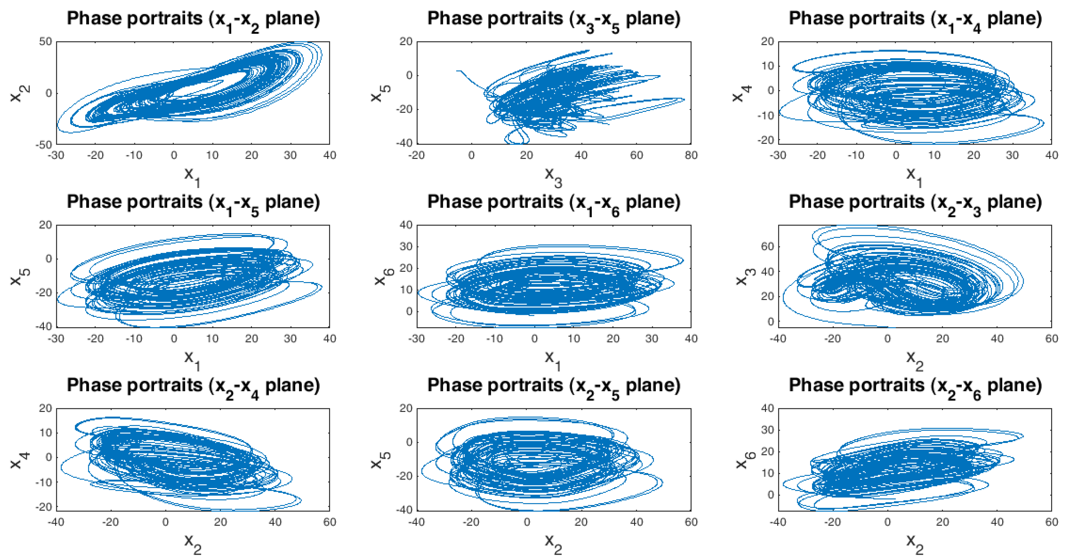
4.1. Introduction and Formulation

In what follows, to prove the effectiveness of the planned controller and hyper-chaotic synchronization, we use a new six-dimensional hyper-chaotic system. All numerical simulations in Section 4.1, Section 4.3 and Section 4.4 were performed with the MATLAB/Simulink toolbox, the ode45 solver, and a step size of 1 ms. The new system is as follows:

$$\begin{gathered} {\dot{x}}_1=a_1\left(x_2-x_1\right)-a_2{x}_5 \\ {\dot{x}}_2=a_3{x}_1-a_4{x}_4-x_1{x}_3 \\ {\dot{x}}_3=-a_5{x}_3+x_1^2 \\ {\dot{x}}_4=a_6\left(x_2+x_5\right)+x_6+k|x_3| \\ {\dot{x}}_5=a_7{x}_2-x_6 \\ {\dot{x}}_6=-a_8{x}_1+a_9\left(x_2+x_4\right)-x_5 \end{gathered}$$

(43)

where $k\in \left(0,5.5\right)$ is a hyper–chaotic control parameter. The hyper–chaotic system (43) has the following initial conditions and parameters:

$$\begin{gathered} x_1\left(0\right)=-0.6, x_2\left(0\right)=2.7, x_3\left(0\right)=-5.4, x_4\left(0\right)=7.3, x_5\left(0\right)=2.4, x_6\left(0\right)=-2, \\ {a}_1=19.8, a_2=1.2, a_3=22, a_4=18.6, a_5=7.5, a_6=3.7, a_7=6.9, a_8=5.3, a_9=0.87 \end{gathered}$$

(44)

Figure 1 displays the 2D phase portraits of the new system (43) with the parameters (44) and three different initial conditions. Figure 2 displays the 2D phase portraits of the new system (43) with the parameters (44) and a different hyper–chaotic control parameter. As it turns out, the new system is sensitive to changes in the initial conditions.

Figure 3 shows Lyapunov exponents of the hyper-chaotic system in exchange for a change in the control parameter $k\in \left(0,5.5\right)$. One of the attractions of the new system is the existence of four positive Lyapunov exponents, which are

$${\mathrm{LE}}_1=1.752, {\mathrm{LE}}_2=1.335,{ \mathrm{LE}}_3=0.958,{ \mathrm{LE}}_4=0.92,{ \mathrm{LE}}_5=0,{ \mathrm{LE}}_6=-1.513$$

(45)

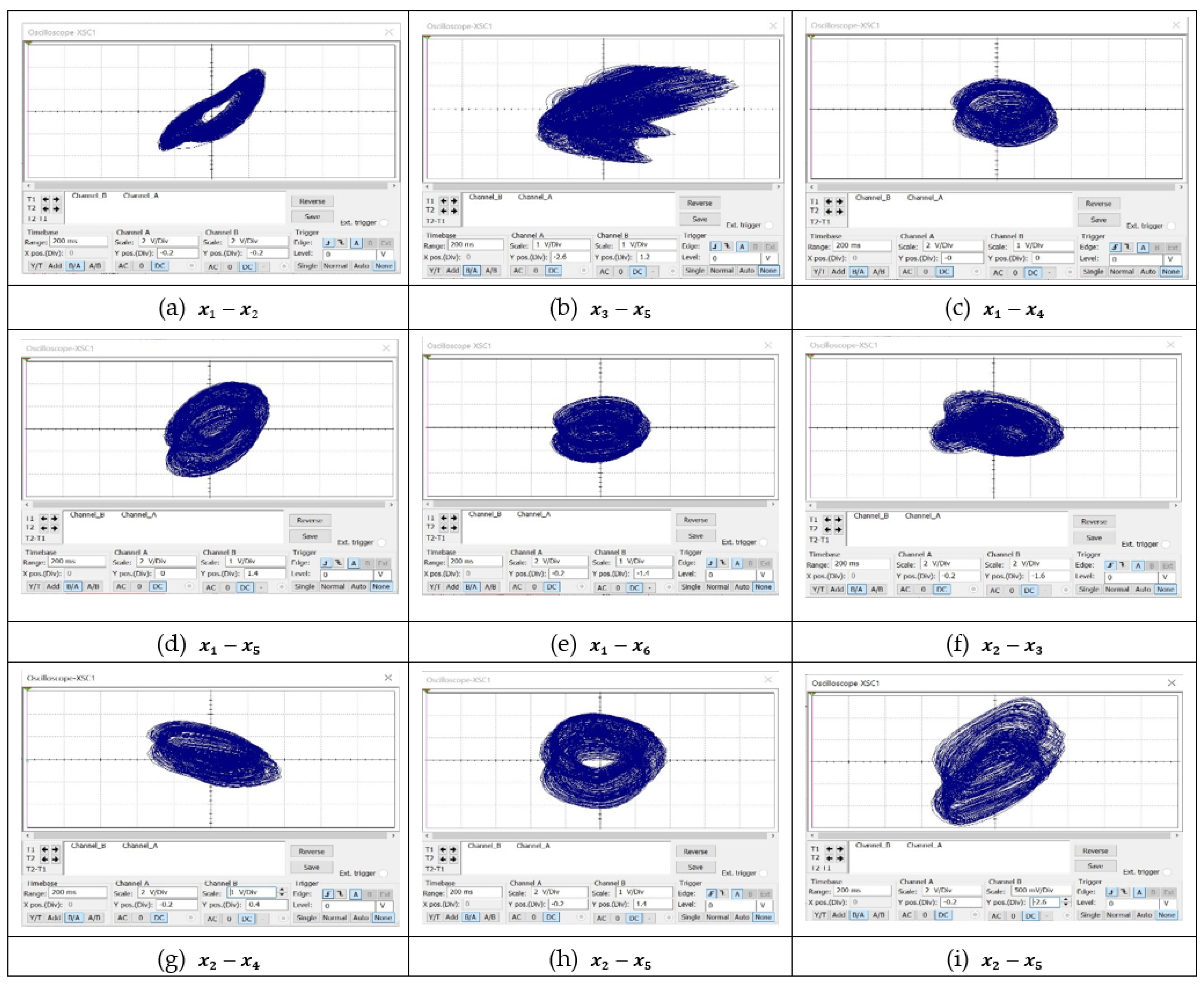
4.2. Circuit Realization of the New Hyperchaotic System

The analog electronic schematic of the new hyper-chaotic system (43) using MultiSIM is given in Figure 4.

The components used in this hyperchaotic circuit include 37 resistors, 6 capacitors, 2 AD633/AD multiplier ICs, 14 op-amps, and 2 1N4148 diodes. By using the Kirchhoff laws of the planned electronic circuit, its nonlinear equations were derived in the subsequent form

$$\begin{gathered} {\dot{x}}_1=\frac{1}{C_1{R}_1}{x}_2-\frac{1}{C_1{R}_2}{x}_1-\frac{1}{C_1{R}_3}{x}_5 \\ {\dot{x}}_2=\frac{1}{C_2{R}_4}{x}_1-\frac{1}{C_2{R}_5}{x}_4-\frac{1}{10C_2{R}_6}{x}_1{x}_3 \\ {\dot{x}}_3=\frac{1}{C_3{R}_7}{x}_3+\frac{1}{10C_3{R}_8}{x}_1^2 \\ {\dot{x}}_4=\frac{1}{C_4{R}_9}{x}_2+\frac{1}{C_4{R}_{10}}{x}_5+\frac{1}{C_4{R}_{11}}{x}_6+\frac{1}{C_4{R}_{12}}|x_3| \\ {\dot{x}}_5=\frac{1}{C_5{R}_{13}}{x}_2-\frac{1}{C_5{R}_{14}}{x}_6 \\ {\dot{x}}_6=-\frac{1}{C_6{R}_{15}}{x}_1+\frac{1}{C_6{R}_{16}}{x}_2+\frac{1}{C_6{R}_{17}}{x}_4-\frac{1}{C_6{R}_{18}}{x}_5 \end{gathered}$$

(46)

where x₁, x₂, x₃, x₄, x₅, and x₆ denote the voltages across capacitors C₁, C₂, C₃, C₄, C₅, and C₆, correspondingly. The following circuit components were selected: R₁ = R₂ = 20.2 kΩ, R₃ = R₁₂ = 333.33 kΩ, R₄ = 18.8 kΩ, R₅ = 21.5 kΩ, R₆ = R₈ = 40 kΩ, R₇ = 53.33 kΩ, R₉ = R₁₀ = 108.11 kΩ, R₁₃ = 57.97 kΩ, R₁₅ = 75.47 kΩ, R₁₈ = 400 kΩ, R₁₆ = R₁₇ = 459.77 kΩ, R₁₉ = R₂₀ = R₂₁ = R₂₂ = R₂₃ = R₂₄ = R₂₅ = R₂₆ = R₂₇ = R₂₈ = R₂₉ = R₃₀ = R₃₁ = R₃₂ = R₃₃ = R₃₄ = R₃₅ = R₃₆ = R₃₇ = 100 kΩ, C₁ = C₂ = C₃ = C₄ = C₅ = C₆ = 1 nF. All active devices were supplied with ±15 Volt and the operational amplifiers TL082CD were employed. The phase portraits on the MultiSIM results are illustrated in Figure 5. The agreement between the numerical results (Figure 6) and MultiSIM results (Figure 5) demonstrates the feasibility of the proposed hyperchaotic system.

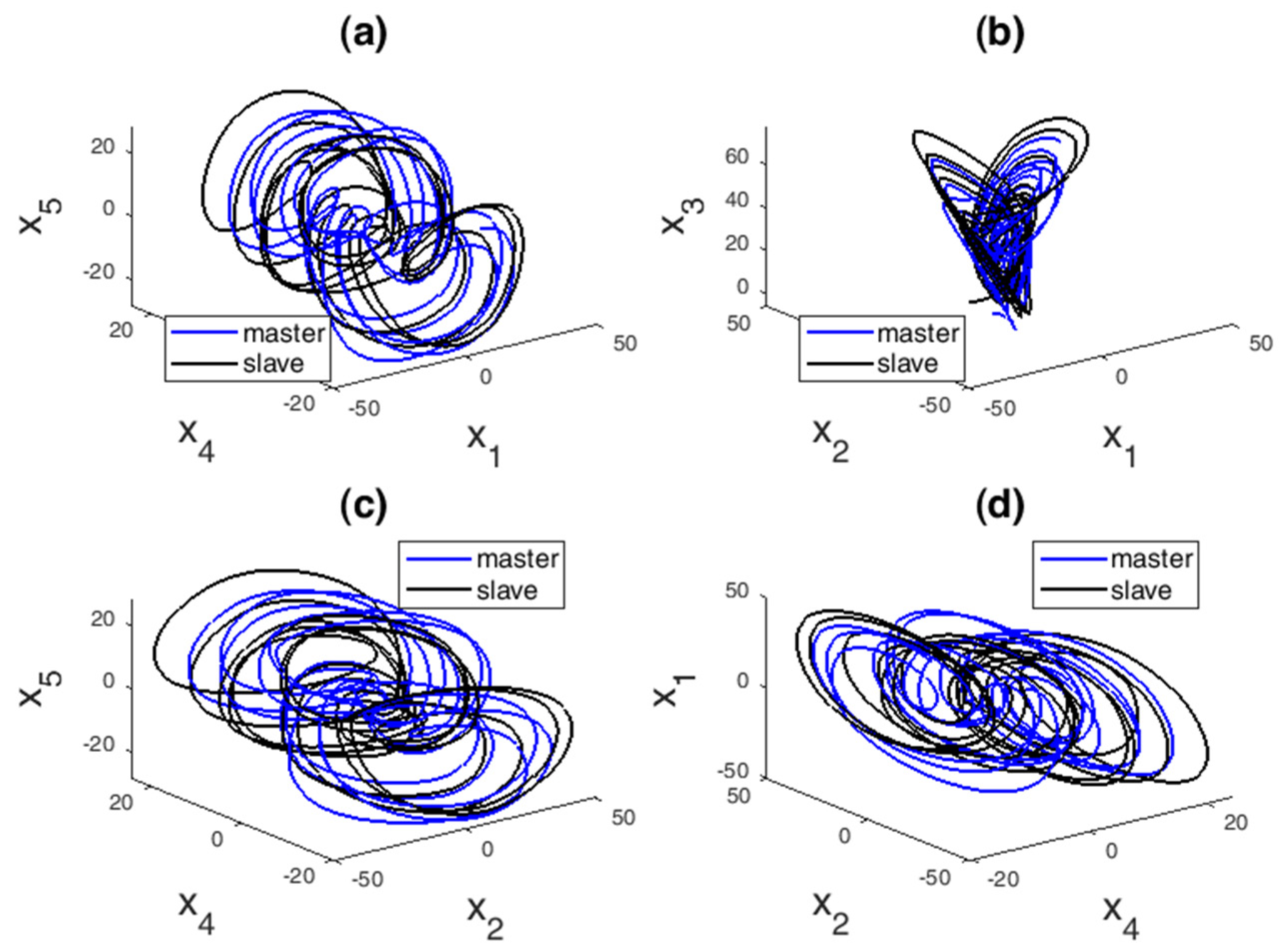
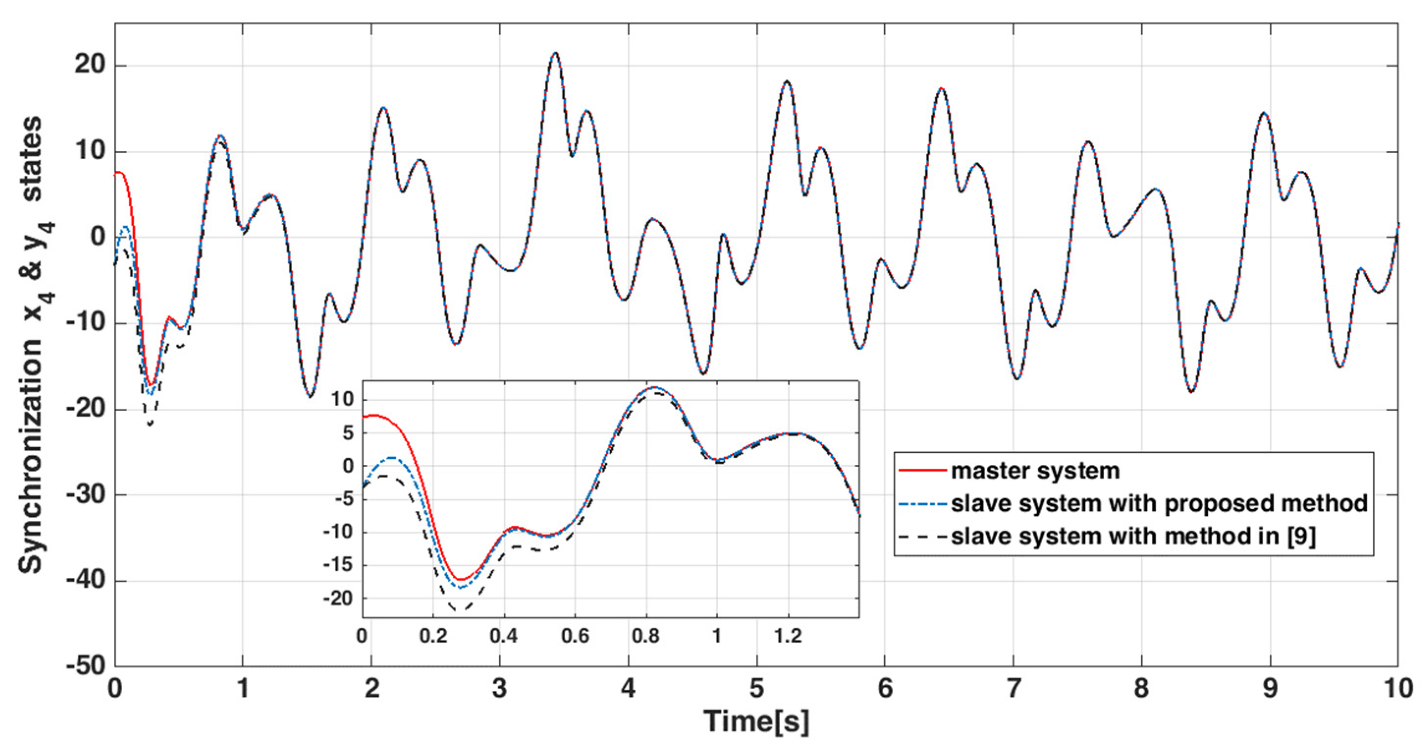
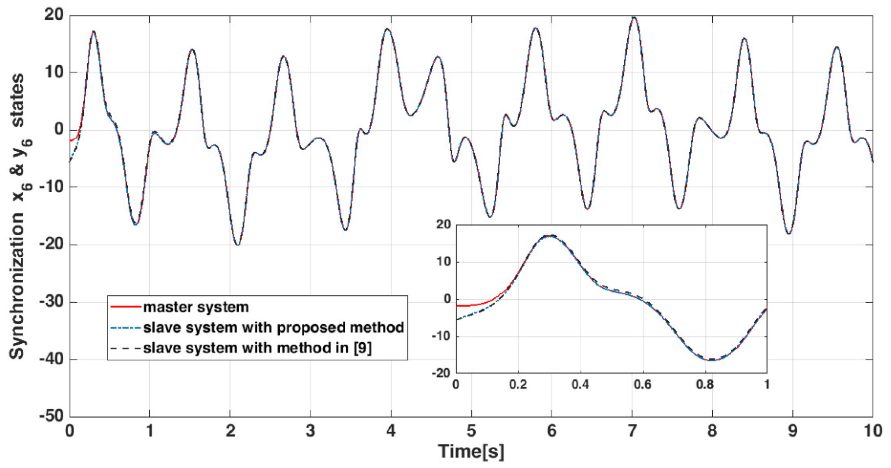
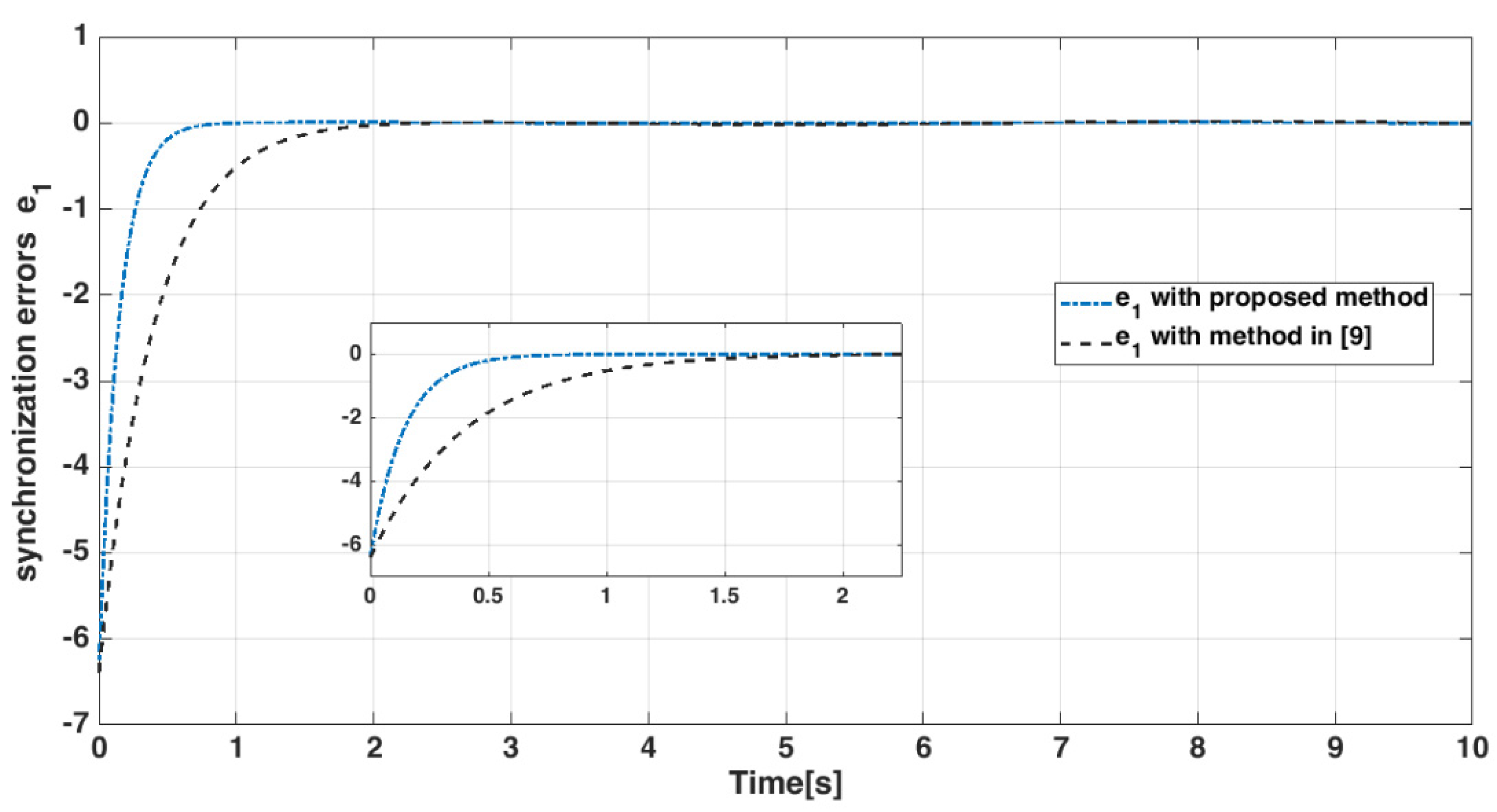
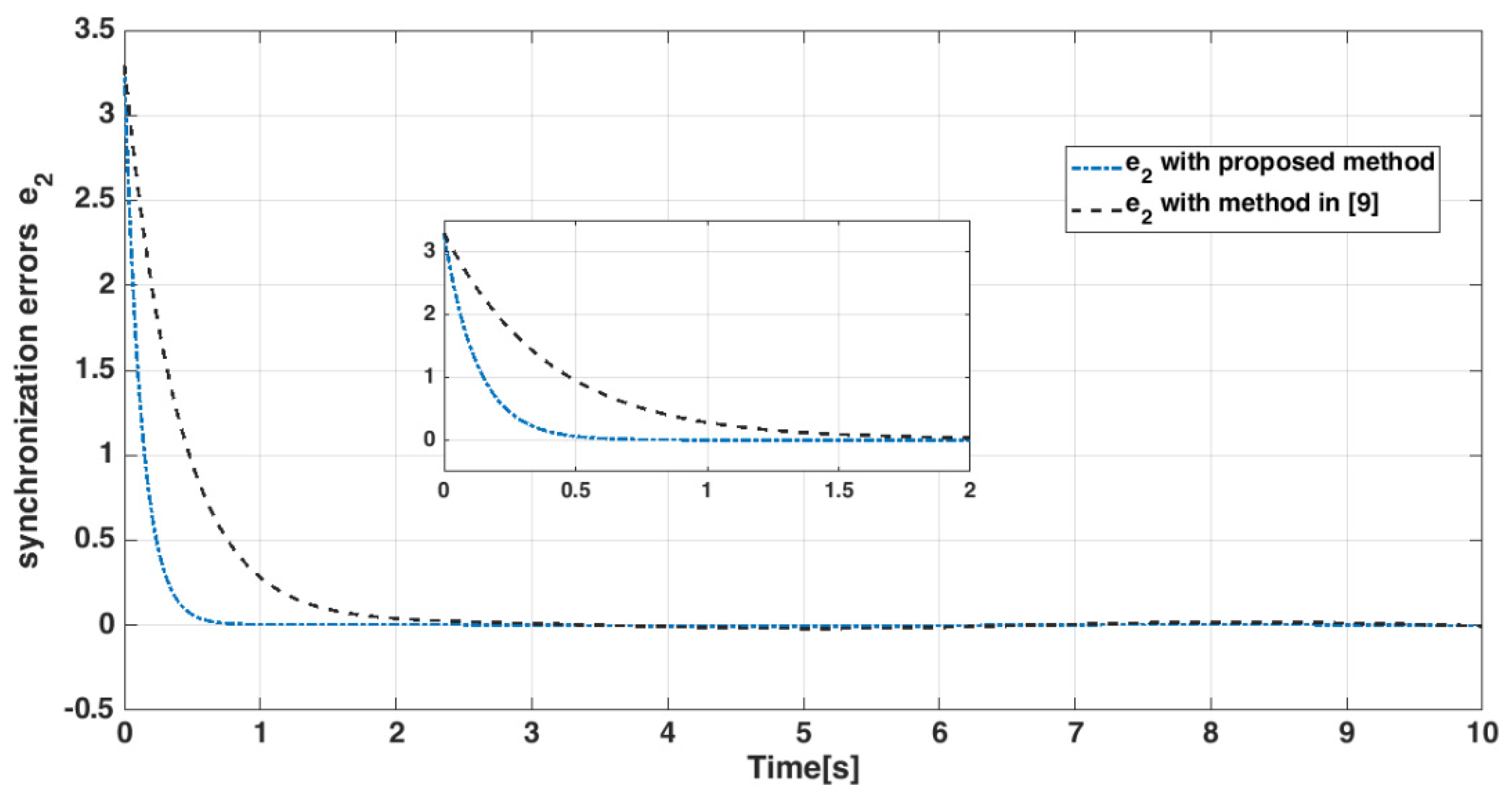
4.3. Hyper-Chaotic Synchronization

For synchronization, we selected the hyper-chaotic system (44) as the master. Similarly, for the hyper-chaotic slave system, we obtained

$$\begin{gathered} {\dot{y}}_1=a_1\left(y_2-y_1\right)-a_2{y}_5+d_1+u \\ {\dot{y}}_2=a_3{y}_1-a_4{y}_4-y_1{y}_3+d_2+u \\ {\dot{y}}_3=-a_5{y}_3+y_1^2+d_3+u \\ {\dot{y}}_4=a_6\left(y_2+y_5\right)+y_6+d_4++k|y_3|+u \\ {\dot{y}}_5=a_7{y}_2-y_6+d_5+u_5 \\ {\dot{y}}_6=-a_8{y}_1+a_9\left(y_2+y_4\right)-y_5+d_6+u \end{gathered}$$

(47)

where the sum of the uncertainty and disturbances is equal to

$$d_i=\left[\begin{array}{c}{d}_1\\ d_2\\ d_3\\ d_4\\ d_5\\ d_6\end{array}\right]=\left[\begin{array}{c}0.2 sin\left(17t\right)+14\\ -0.5 cos\left(20t\right)+10\\ -1.2 sin\left(13t\right)+2.8\\ 2 cos\left(11t\right)-7.2\\ 16 sin\left(2.4t\right)-12\\ 5 cos\left(14t\right)+24\end{array}\right]$$

(48)

Figure 7 demonstrates the 3-D phase portraits of master-slave systems (43) and (47) without controller. As it turns out, the systems behave differently.

Definition 3.

The master-slave systems (43) and (47) can be synchronized in a limited time $\tau$ [42]:

$$\underset{t\to \tau }{lim}\Vert y_j-x_j\Vert =0, j=1,2,\dots ,N$$

(49)

Assumption 2.

Suppose  $y_i\left(\tau \right)=x_i\left(\tau \right)$ implies that $\underset{\tau \to \infty }{lim}{e}_i\left(\tau \right)$.

Assumption 3.

Let the finite–time synchronization errors of systems (43) and (47) be defined as: $e_i=y_i-x_i , i=1,\dots ,6$.

Based on Assumption 3, to study chaos synchronization, the error according to systems (43) and (47) can be designed as follows:

$$\begin{gathered} {\dot{e}}_1=a_1\left(e_2-e_1\right)-a_2{e}_4+d_1+u \\ {\dot{e}}_2=a_3{e}_1-a_4{e}_4-y_1{y}_3+x_1{x}_3+d_2+u \\ {\dot{e}}_3=-a_5{e}_1+y_1^2-x_1^2+d_3+u \\ {\dot{e}}_4=a_6\left(e_2+e_5\right)+e_6+d_4+u \\ {\dot{e}}_5=a_7{e}_2-e_6+d_5+u \\ {\dot{e}}_6=-a_8{e}_1+a_9\left(e_2-e_4\right)-e_5+d_6+u \end{gathered}$$

(50)

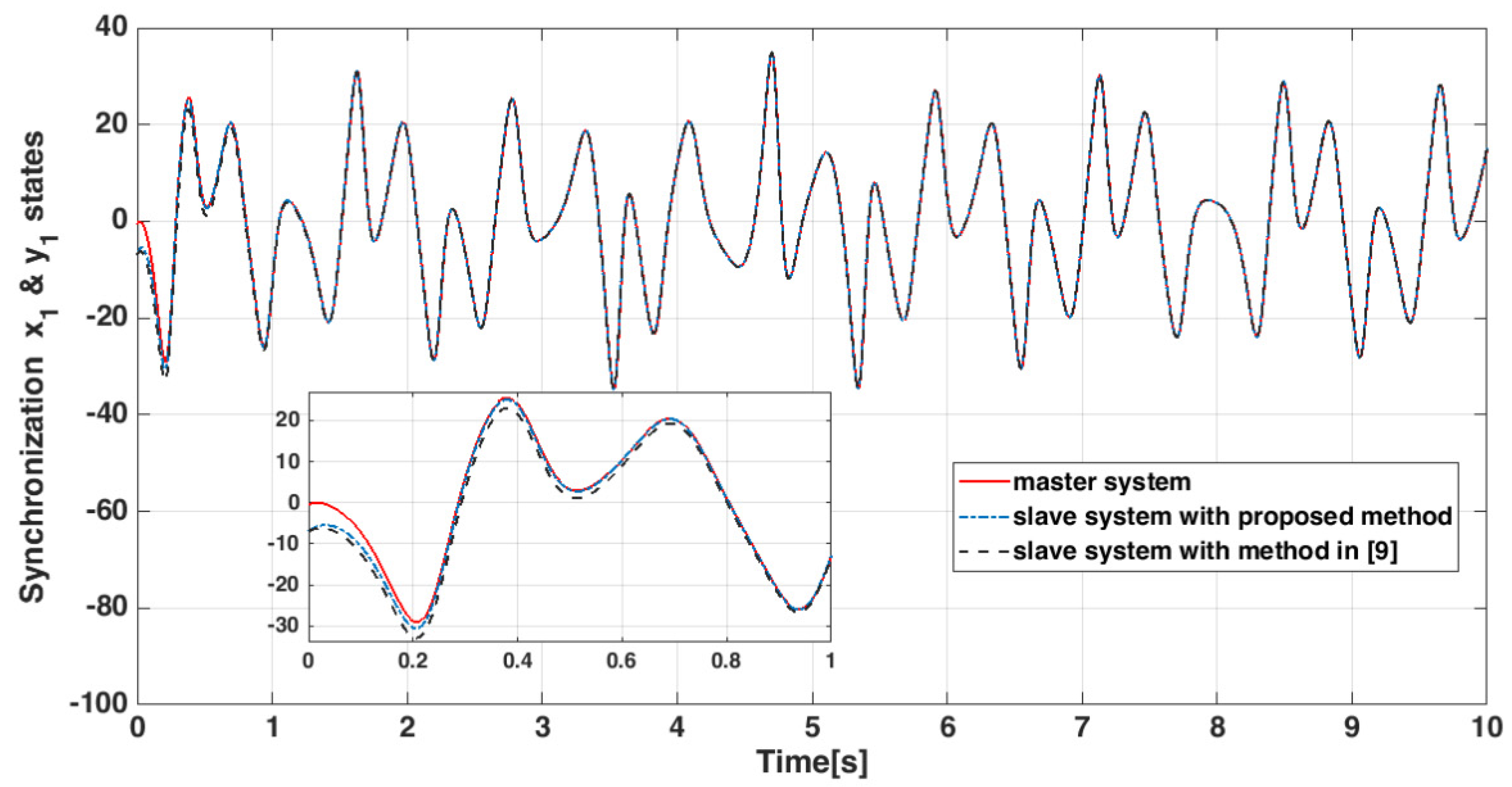
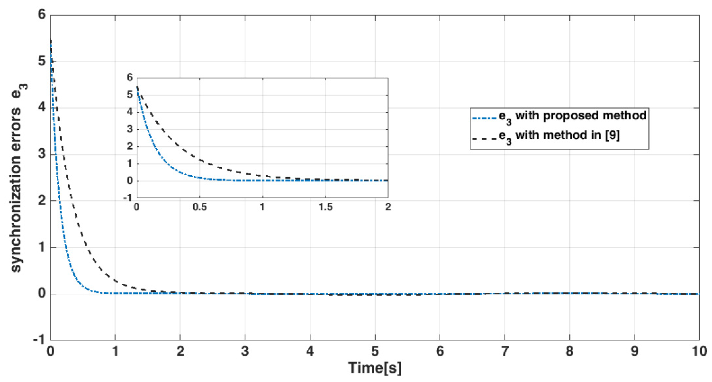
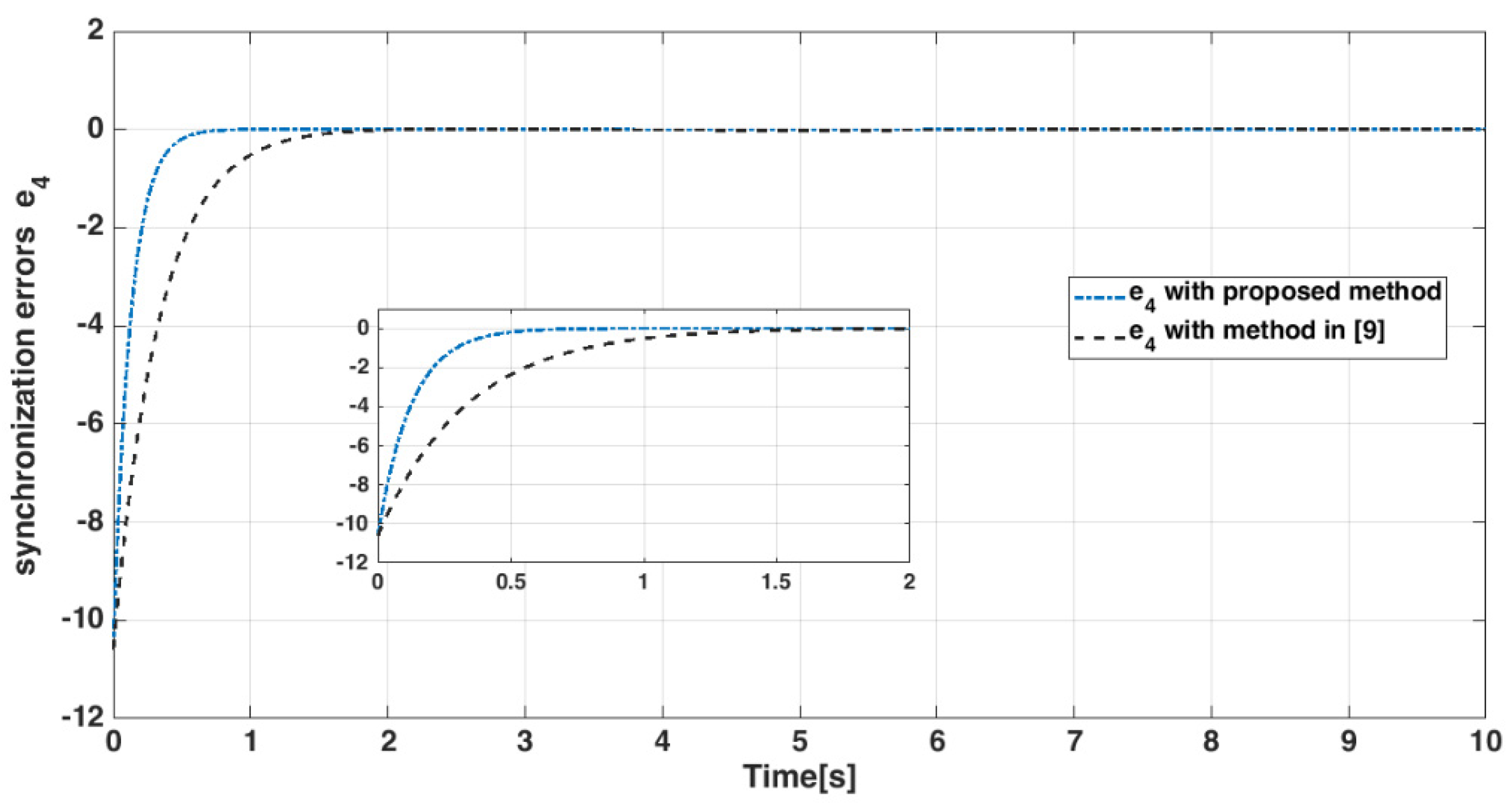
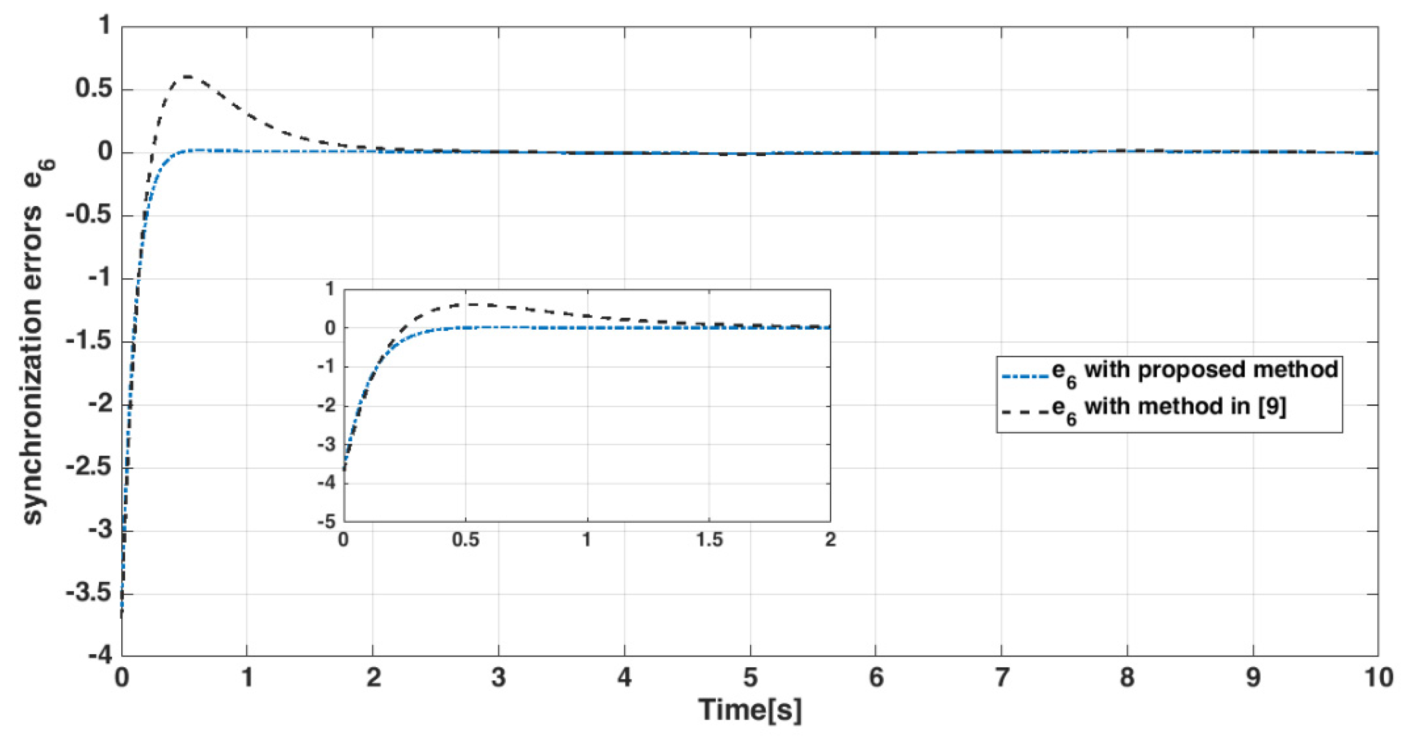
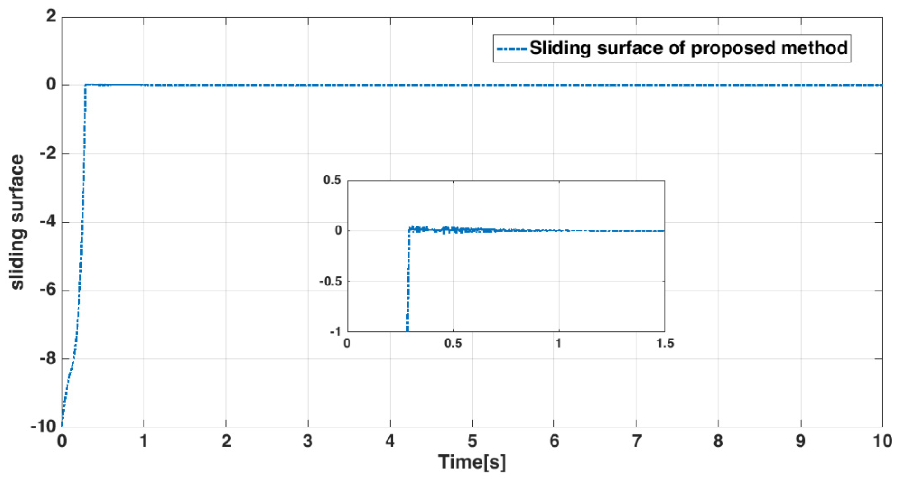
4.4. Numerical Results

In what follows, for hyper-chaotic finite-time synchronization, two simulator master-slave systems (43) and (47) using MATLAB software are presented. For finite-time synchronization, we used the accepted integral-type controller (36). In order to confirm the planned technique, all outcomes of this article are compared with the results of the planned method presented in [9]. For this purpose, we selected the controller parameters as follows:

$$\begin{gathered} k_p=\left[1.32 0.708 2.26 0.02 3.04 1.08\right] \\ {k}_d=\left[0.04 0.32 4.06 3.9 7.1 0.05\right] k_i=\left[2.6 1.3 5 1 0.9 0.04\right] \\ \kappa =32, \gamma =0.22, \eta =7/9 \end{gathered}$$

(51)

Increasing or decreasing the convergence speed, tracking accuracy, and the control signal amplitude depends on having the proper settings for the parameters $k_p$, $k_i$ and $k_d$. Increasing or decreasing the tracking accuracy and convergence rate depends on having the proper settings for the parameters $\kappa$, $\gamma$, and $\eta$. Additionally, having an excessive increase or improper adjustment of these three parameters can increase the amplitude of the control signal, causing the chattering phenomenon.

The state responses of the hyper-chaotic master-slave systems (43) and (47) compared to the method presented in [9], are shown from Figure 8, Figure 9, Figure 10, Figure 11, Figure 12 and Figure 13.

The state trajectories of the error dynamic systems $e_1-e_6$ compared to the method presented in [9], are shown from Figure 14, Figure 15, Figure 16, Figure 17, Figure 18 and Figure 19. According to the figures, it is obvious that the error system converges to the origin in finite time. Therefore, finite-time synchronization has occurred, and the proposed controller can eliminate uncertainties in a finite-time with better resistance.

In Figure 20, the control inputs are compared to the method presented in [9]. The time histories of the sliding surface are shown in Figure 21. As it turns out, the controller designed in this article has less overshoot than a similar controller.

Based on the above outcomes, the planned control scheme is able to stabilize the master-slave systems in finite time and achieves a good tracking performance while also eliminating the chattering phenomenon.

5. Conclusions

This study planned a novel nonsingular integral terminal sliding control strategy for finite-time synchronization of a category of hyper-chaotic systems. Then, an integral sliding mode control input was suggested to synchronize hyper-chaotic systems. Using the Lyapunov stability theorem, the planned controller scheme confirmed that master-slave hyper-chaotic systems arrive in the existence of parameter uncertainty as quickly as possible. To prove the applicability of the proposed controller, a new six-dimensional hyper-chaotic system in the form of two master-slave subsystems was used. The planned method satisfied the requirements of finite-time synchronization and properly alleviated uncertainty while attenuating the chattering phenomenon effect. The circuit realization of the new hyperchaotic system and simulation outcomes related to the implementation of the recommended technique on the considered hyperchaotic systems were studied. The proposed design method does not consider the actuator errors, and this will be realized in future work. It is also recommended to use nonsingular integral-type controllers in power systems, especially permanent-magnet electric motors. For the future research, we will focus on applications with time-varying disturbances, where the switching controllers can be employed to reduce the operating costs.

References

1. Mahmoud, E.E.; Jahanzaib, L.S.; Trikha, P.; Abualnaja, K.M. Analysis and control of a fractional chaotic tumour growth and decay model. Results Phys. 2021, 20, 103677. [Google Scholar] [CrossRef]
2. Iqbal, S.A.; Hafez, M.; Karim, S.A.A. Bifurcation analysis with chaotic motion of oblique plane wave for describing a discrete nonlinear electrical transmission line with conformable derivative. Results Phys. 2020, 18, 103309. [Google Scholar] [CrossRef]
3. Guo, R.; Zhang, Y.; Jiang, C. Synchronization of Fractional-Order Chaotic Systems with Model Uncertainty and External Disturbance. Mathematics 2021, 9, 877. [Google Scholar] [CrossRef]
4. Lin, C.-H.; Ho, C.-W.; Hu, G.-H.; Sreeramaneni, B.; Yan, J.-J. Secure Data Transmission Based on Adaptive Chattering-Free Sliding Mode Synchronization of Unified Chaotic Systems. Mathematics 2021, 9, 2658. [Google Scholar] [CrossRef]
5. Li, Y.; Li, Z.; Ma, M.; Wang, M. Generation of grid multi-wing chaotic attractors and its application in video secure communication system. Multimed. Tools Appl. 2020, 79, 29161–29177. [Google Scholar] [CrossRef]
6. Zhu, B.; Wang, F.; Yu, J. A Chaotic Encryption Scheme in DMT for IM/DD Intra-Datacenter Interconnects. IEEE Photon. Technol. Lett. 2021, 33, 383–386. [Google Scholar] [CrossRef]
7. Simhanath, Y. Religious Nationalism as Solution in the Chaotic Social, Economics and the Business Reality. Int. J. Relig. Cult. Stud. 2020, 2, 25–29. [Google Scholar] [CrossRef]
8. Weinmeister, J.; Xie, N.; Gao, X.; Prasad, A.K.; Roy, S. Analysis of a Polynomial Chaos-Kriging Metamodel for Uncertainty Quantification in Aerospace Applications. In Proceedings of the AIAA/ASCE/AHS/ASC Structures, Structural Dynamics, and Materials Conference, Kissimmee, FL, USA, 8–12 January 2018. [Google Scholar] [CrossRef] [Green Version]
9. Li, Y.-X.; Yang, G.-H. Adaptive integral sliding mode control fault tolerant control for a class of uncertain nonlinear systems. IET Control Theory Appl. 2018, 12, 1864–1872. [Google Scholar] [CrossRef]
10. Mahmoud, E.E.; Al-Harthi, B.H. A phenomenal form of complex synchronization and chaotic masking communication between two identical chaotic complex nonlinear structures with unknown parameters. Results Phys. 2019, 14, 102452. [Google Scholar] [CrossRef]
11. Sha, D.; Ozbay, K.; Bian, Z.; Wang, D. A Polynomial Chaos Expansion Based Approach for Efficient and Robust Calibration of Stochastic Transportation Simulation Models. In Proceedings of the Transportation Research Board 100th Annual Meeting, Washington, DC, USA, 5–29 January 2021. [Google Scholar]
12. Avanço, R.H.; Tusset, A.M.; Balthazar, J.M.; Nabarrete, A.; Navarro, H.A. On nonlinear dynamics behavior of an electro-mechanical pendulum excited by a nonideal motor and a chaos control taking into account parametric errors. J. Braz. Soc. Mech. Sci. Eng. 2018, 40, 23. [Google Scholar] [CrossRef]
13. Lu, S.; Wang, X.; Wang, L. Finite-time adaptive neural network control for fractional-order chaotic PMSM via command filtered backstepping. Adv. Differ. Equ. 2020, 2020, 121. [Google Scholar] [CrossRef] [Green Version]
14. Gunasekaran, N.; Joo, Y.H. Stochastic sampled-data controller for T–S fuzzy chaotic systems and its applications. IET Control Theory Appl. 2019, 13, 1834–1843. [Google Scholar] [CrossRef]
15. Gunasekaran, N.; Srinivasan, S.; Zhai, G.; Yu, Q. Dynamical Analysis and Sampled-Data Stabilization of Memristor-Based Chua’s Circuits. IEEE Access 2021, 9, 25648–25658. [Google Scholar] [CrossRef]
16. Morales, G.B.; Muñoz, M.A. Optimal Input Representation in Neural Systems at the Edge of Chaos. Biology 2021, 10, 702. [Google Scholar] [CrossRef]
17. Abanin, D.A.; Bardarson, J.H.; De Tomasi, G.; Gopalakrishnan, S.; Khemani, V.; Parameswaran, S.A.; Pollmann, F.; Potter, A.C.; Serbyn, M.; Vasseur, R. Distinguishing localization from chaos: Challenges in finite-size systems. Ann. Phys. 2021, 427, 168415. [Google Scholar] [CrossRef]
18. Taylor, L. The taming of chaos: Optimal cities and the state of the art in urban systems research. Urban Stud. 2021, 58, 3196–3202. [Google Scholar] [CrossRef]
19. Kos, P.; Bertini, B.; Prosen, T. Chaos and Ergodicity in Extended Quantum Systems with Noisy Driving. Phys. Rev. Lett. 2021, 126, 190601. [Google Scholar] [CrossRef]
20. Gunasekaran, N.; Joo, Y.H. Robust Sampled-data Fuzzy Control for Nonlinear Systems and Its Applications: Free-Weight Matrix Method. IEEE Trans. Fuzzy Syst. 2019, 27, 2130–2139. [Google Scholar] [CrossRef]
21. Gunasekaran, N.; Saravanakumar, R.; Ali, M.S.; Zhu, Q. Exponential sampled-data control for T–S fuzzy systems: Application to Chua’s circuit. Int. J. Syst. Sci. 2019, 50, 2979–2992. [Google Scholar] [CrossRef]
22. Xian, Y.-J.; Xia, C.; Guo, T.-T.; Fu, K.-R.; Xu, C.-B. Dynamical analysis and FPGA implementation of a large range chaotic system with coexisting attractors. Results Phys. 2018, 11, 368–376. [Google Scholar] [CrossRef]
23. Pecora, L.M.; Carroll, T.L. Synchronization in chaotic systems. Phys. Rev. Lett. 1990, 64, 821. [Google Scholar] [CrossRef]
24. Rahman, Z.-A.S.A.; Jasim, B.H.; Al-Yasir, Y.I.A.; Hu, Y.-F.; Abd-Alhameed, R.A.; Alhasnawi, B.N. A New Fractional-Order Chaotic System with Its Analysis, Synchronization, and Circuit Realization for Secure Communication Applications. Mathematics 2021, 9, 2593. [Google Scholar] [CrossRef]
25. Akinlar, M.A.; Tchier, F.; Inc, M. Chaos control and solutions of fractional-order Malkus waterwheel model. Chaos Solitons Fractals 2020, 135, 109746. [Google Scholar] [CrossRef]
26. Yan, L.; Liu, J.; Xu, F.; Teo, K.L.; Lai, M. Control and synchronization of hyperchaos in digital manufacturing supply chain. Appl. Math. Comput. 2021, 391, 125646. [Google Scholar] [CrossRef]
27. Batmani, Y. Chaos control and chaos synchronization using the state-dependent Riccati equation techniques. Trans. Inst. Meas. Control. 2018, 41, 311–320. [Google Scholar] [CrossRef]
28. Bartolini, G.; Ferrara, A.; Levant, A.; Usai, E. On second order sliding mode controllers. In Variable Structure Systems, Sliding Mode and Nonlinear Control; Young, K., Özgüner, Ü., Eds.; Springer: London, UK, 1999; Volume 247, pp. 329–350. Available online: https://link.springer.com/chapter/10.1007/BFb0109984#citeas (accessed on 20 November 2021).
29. Boiko, I.; Fridman, L. Analysis of chattering in continuous sliding-mode controllers. IEEE Trans. Autom. Control. 2005, 50, 1442–1446. [Google Scholar] [CrossRef] [Green Version]
30. Liu, J.; Wang, X. Advanced Sliding Mode Control for Mechanical Systems; Springer: Berlin/Heidelberg, Germany, 2011. [Google Scholar] [CrossRef]
31. Shtessel, Y.; Edwards, C.; Fridman, L.; Levant, A. Sliding Mode Control and Observation; Springer: New York, NY, USA, 2014; Volume 10. [Google Scholar]
32. Yang, J.; Su, J.; Li, S.; Yu, X. High-Order Mismatched Disturbance Compensation for Motion Control Systems Via a Continuous Dynamic Sliding-Mode Approach. IEEE Trans. Ind. Inform. 2013, 10, 604–614. [Google Scholar] [CrossRef] [Green Version]
33. Qiao, L.; Zhang, W. Adaptive non-singular integral terminal sliding mode tracking control for autonomous underwater vehicles. IET Control. Theory Appl. 2017, 11, 1293–1306. [Google Scholar] [CrossRef]
34. Mobayen, S.; Karami, H.; Fekih, A. Adaptive Nonsingular Integral-type Second Order Terminal Sliding Mode Tracking Controller for Uncertain Nonlinear Systems. Int. J. Control Autom. Syst. 2021, 19, 1539–1549. [Google Scholar] [CrossRef]
35. Rashidnejad, Z.; Karimaghaee, P. Synchronization of a class of uncertain chaotic systems utilizing a new finite-time fractional adaptive sliding mode control. Chaos Solitons Fractals X 2020, 5, 100042. [Google Scholar] [CrossRef]
36. Tong, D.; Xu, C.; Chen, Q.; Zhou, W. Sliding mode control of a class of nonlinear systems. J. Frankl. Inst. 2020, 357, 1560–1581. [Google Scholar] [CrossRef]
37. Shukla, M.K.; Sharma, B.B. Control and Synchronization of a Class of Uncertain Fractional Order Chaotic Systems via Adaptive Backstepping Control. Asian J. Control 2017, 20, 707–720. [Google Scholar] [CrossRef]
38. Wang, Z.; Li, Q.; Li, S. Adaptive Integral-Type Terminal Sliding Mode Fault Tolerant Control for Spacecraft Attitude Tracking. IEEE Access 2019, 7, 35195–35207. [Google Scholar] [CrossRef]
39. Yang, Y. A time-specified nonsingular terminal sliding mode control approach for trajectory tracking of robotic airships. Nonlinear Dyn. 2018, 92, 1359–1367. [Google Scholar] [CrossRef]
40. Dinga, S.; Park, J.H.; Chenc, C.C. Second-order sliding mode controller design with output constraint. Automatica 2020, 112, 108704. [Google Scholar] [CrossRef]
41. Zhang, X. Robust integral sliding mode control for uncertain switched systems under arbitrary switching rules. Nonlinear Anal. Hybrid Syst. 2020, 37, 100900. [Google Scholar] [CrossRef]
42. Abdurahman, A.; Jiang, H.; Teng, Z. Finite-time synchronization for memristor-based neural networks with time-varying delays. Neural Netw. 2015, 69, 20–28. [Google Scholar] [CrossRef]
Figure 1. Phase portrait diagrams of the new hyper-chaotic system on the x 2 x 3 space for different initial conditions: (a) [−0.01, −0.1, −0.01, −0.1, −0.01, −2.5], (b) [−0.1, −0.1, −0.1, −2.5, −0.1, −0.1] and (c) [−0.1, −0.1, −0.1, −0.1, −0.1, −2.5].
Mathematics 10 00115 g001
Figure 2. Phase portrait diagrams of the new hyper-chaotic system on the x 1 x 2 space for different hyper–chaotic control parameters: (a) [k = 0.002], (b) [k = 0.2], (c) [k = 0.85] and (d) [k = 1].
Mathematics 10 00115 g002
Figure 3. Lyapunov exponent spectrum of the new system (43) in k ( 0 , 5.5 ) .
Mathematics 10 00115 g003
Figure 4. Circuit realization of the new hyperchaotic system (43).
Mathematics 10 00115 g004aMathematics 10 00115 g004b
Figure 5. MultiSIM hyperchaotic attractors of the new chaotic system (43): (a) x1x2; (b) x3x5; (c) x1x4; (d) x1x5; (e) x1x6; (f) x2x3; (g) x2x4; (h) x2x5; (i) x2x5.
Mathematics 10 00115 g005
Figure 6. MATLAB PLOT hyperchaotic attractors of the new chaotic system (43).
Mathematics 10 00115 g006
Figure 7. Three-dimensional phase portraits of the master system (43) with the initial conditions (44) and the slave system (47) with the initial conditions [ y 1 ( 0 ) , y 2 ( 0 ) , y 3 ( 0 ) , y 4 ( 0 ) , y 5 ( 0 ) , y 6 ( 0 ) ] = [ 7 ,   6 ,   0.1 , 3.3 ,   1.4 , 5.7 ] in the (a) x 1 x 4 x 5 plane, (b) x 1 x 2 x 3 plane, (c) x 2 x 4 x 5 plane, and (d) x 4 x 2 x 1 plane.
Mathematics 10 00115 g007
Figure 8. Time trajectories of states x 1 and y 1 .
Mathematics 10 00115 g008
Figure 9. Time responses of states x 2 and y 2 .
Mathematics 10 00115 g009
Figure 10. Time responses of states x 3 and y 3 .
Mathematics 10 00115 g010
Figure 11. States x 4 and y 4 .
Mathematics 10 00115 g011
Figure 12. States x 5 and y 5 .
Mathematics 10 00115 g012
Figure 13. States x 6 and y 6 .
Mathematics 10 00115 g013
Figure 14. State error e 1 of master-slave systems.
Mathematics 10 00115 g014
Figure 15. State error e 2 of master-slave systems.
Mathematics 10 00115 g015
Figure 16. State errors e 3 of master-slave systems.
Mathematics 10 00115 g016
Figure 17. State error e 4 of master-slave systems.
Mathematics 10 00115 g017
Figure 18. State error e 5 of master-slave systems.
Mathematics 10 00115 g018
Figure 19. State error e 6 of master-slave systems.
Mathematics 10 00115 g019
Figure 20. Control signal u ( t ) .
Mathematics 10 00115 g020
Figure 21. Integral-type terminal sliding surface s ( e ( t ) ) .
Mathematics 10 00115 g021
Publisher’s Note: MDPI stays neutral with regard to jurisdictional claims in published maps and institutional affiliations.