Optimization Environment Definition for Beam Steering Reflectarray Antenna Design

Abstract

Reflectarray antennas are low-profile high-gain systems widely applied in the aerospace industry. The increase in their application is leading to the problem of getting more advanced performance while keeping the system as simple as possible. In these cases, their design cannot be conducted via analytical methods, thus evolutionary optimization algorithms are often implemented. Indeed, the design is characterized by the presence of many local minima, by high number of design variables, and by the high computational burden required to evaluate the antenna performance. The purpose of this paper is to develop, implement, and test a complete Optimization Environment that can be applied to achieve high scanning capabilities with a reflectarray. The design of the optimization environment has been selected to be flexible enough to be applied also with other different algorithms.

1. Introduction

In recent years, Evolutionary Algorithms (EAs) have been successfully applied to many engineering problems thanks to their capability to find optimal solutions in non-linear and multimodal problems [1]. Another important aspect of EAs is their flexibility: similar frameworks can be applied to different engineering problems [2].

Most of the problems faced with EAs require complex models to simulate the system and to define performance parameters. The model complexity, required for providing an accurate output of the optimization process, is usually time expensive; consequently, it requires an effective optimization process management to achieve the optimal result in reasonable time [3].

The design optimization of Reflectarray Antennas (RAs) is a clear example of this problem: in fact, these systems are composed by hundreds or even thousands of elements that can be optimized, leading to a very large non-linear multimodal optimization problem [4]. RAs are a group of powerful and efficient high-gain antennas; they are highly adopted in many different conditions thanks to their numerous advantages, such as low profile, low cost, good radiation performance, and ease of manufacturing [5]. Compared to traditional phased arrays, RA have a less complex feeding system and, thus, lead to a reduction in the losses introduced by the feeding networks [6].

Among all the antenna configurations, reflector antennas have been exploited for the high demand of radar and satellite communication, where a point-to-point connection was needed and, consequently, a high gain was required. In order to reduce the space required by the reflector, Reflectarray Antennas have been introduced, especially in aerospace applications: in fact, they have low weight, low profile, and the possibility to be easily folded [7]. Reflectarray Antennas consist in a planar array made up of different re-radiating elements illuminated by a feed source (typically a horn antenna) placed in central or offset position. In these antennas, changing one or more geometrical parameter of each patch is used to control the phase of the re-radiated field changes and to obtain the desired radiation pattern [8].

The design process complexity for RA depends on the type of radiation pattern that is required: for the simple case of a pencil beam RA, the design can be carried out analytically [9]. In the case of more complex requirements in terms of radiation pattern, optimization methods are fundamental. In this context, Evolutionary Algorithms (EAs) are very valuable tools.

Genetic Algorithms (GAs) have been widely adopted in the field of reflectarray optimization. In [10] the authors propose the application of GA to create the reflection layer of an RA: with respect to other works, in this one the reflection element shape is not fixed and can be tuned with the GA. A similar approach has been implemented in [11] for a dual band RA. In [12], a reconfigurable RA composed by a two layer pixel patches is proposed. The second layer height can be mechanically adjustable to change the beam direction. Both the pixel patches are optimized by means of a binary GA.

Other EAs have been applied to this problem: for example, Particle Swarm Optimization has been implemented in [13] to design a dual band RA and also Differential Evolution has been applied for the design of RAs [14]. In order to improve the optimization performance, variations of known algorithms are proposed: in [15] an dynamic clustering process is introduced in PSO to improve the trade-off between exploration and exploitation. The application of a single algorithm is not always sufficient due to the problem complexity: for this reason, hybrid approaches have been proposed in literature. The first tested hybridization consists in the combination of GA and PSO [16], while further improvements can be achieved combining EAs with deterministic methods, like the Taguchi one [17,18]. Finally, local search techniques can be applied for the final refinement of the solutions found by the EA. This approach has been applied successfully in [19] for a single optimization problem and in [20] for a multi-objective one.

A recent problem in reflectarray antenna design is to improve their scanning capabilities, i.e., the possibility to modify the direction of the radiation pattern main beam [21]. In our paper this capability is achieved by steering the feeder with respect to a fixed reflector. Thus, the latter must be designed to reach good reflection proprieties with different scan angles. This system is much simpler than electronic scanning, because it does not require a complex biasing system for the reflector; however, the radiation pattern worsens quickly with increasing scan angles. The lack of optimal deterministic solutions to this problem make it suitable to be addressed by an Evolutionary Optimization approach.

The aim of this paper is to analyze the entire Optimization Environment that has been implemented for the design of a beam-scanning RA. The problem is characterized by a large number of design variables (148) and is highly non-linear. The Optimization Environment has been designed to be easily adaptable to different EA: to prove this, seven EAs have been tested on this problem. With respect to other papers available in literature, here the entire optimization process has been analyzed to maximize the EAs performances.

The paper is structured as follows: in Section 2 the optimization problem is described and the optimization environment presented. Section 3 presents a brief description of the adopted Evolutionary Algorithms. In Section 4, the results of the antenna optimization are presented and, finally, in Section 5 some conclusions are drawn.

2. Antenna and Optimization Environment Description

In this section, the analyzed optimization problem will be deeply described. In particular, the antenna is analyzed and then, accordingly to the specific features of the analyzed problem, the optimization environment is properly designed and described.

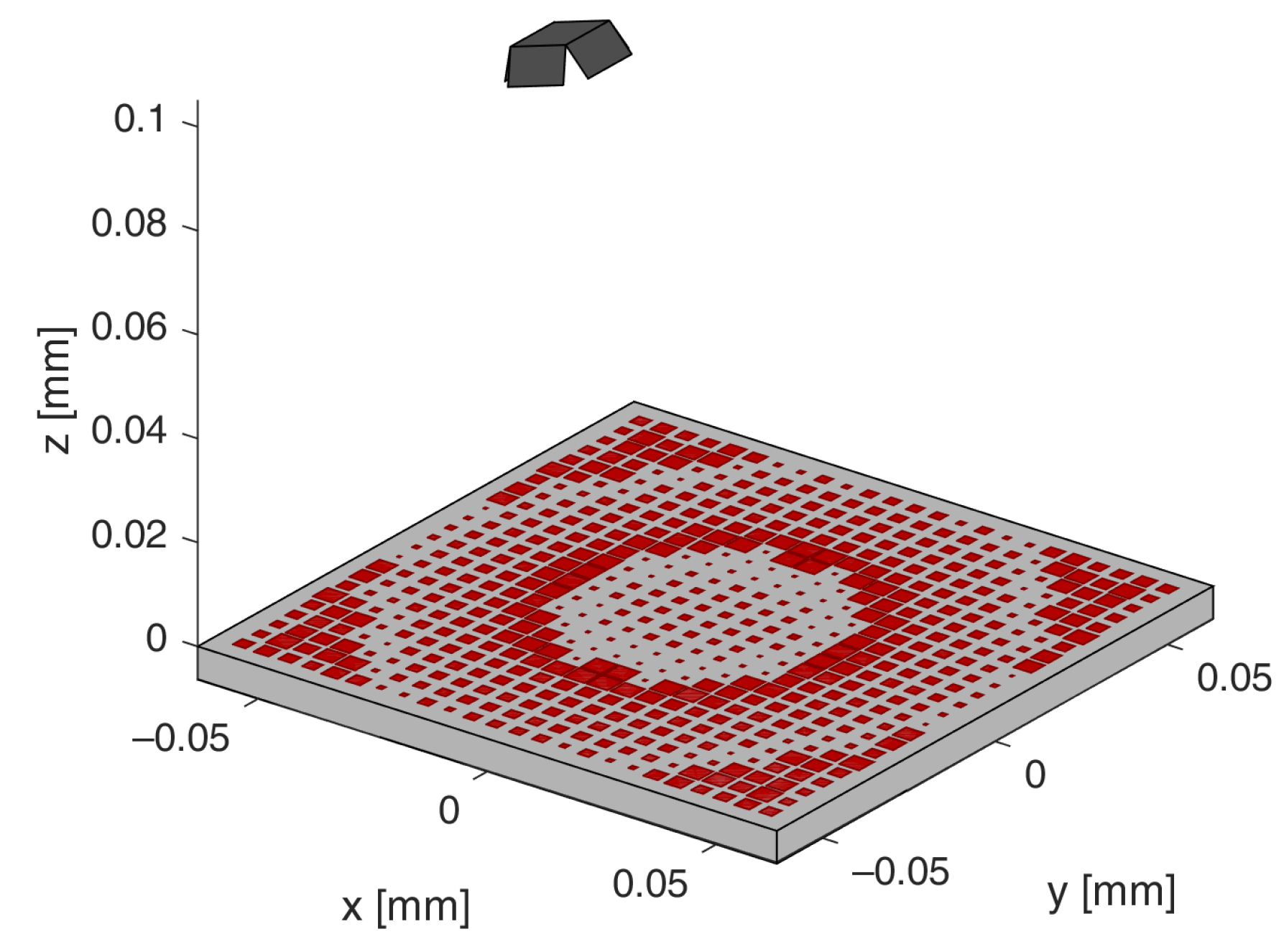
2.1. Antenna Geometry

Reflectarrays (RAs) are antenna structures originally aimed to improve directivity. They consist of a low profile planar array of printed radiating elements illuminated by a primary feed source [22].

Usually these antennas are characterized by a flat reflector: this solution reduces the production costs and the antenna volume which represents an important aspect especially in aerospace applications. Moreover, with respect to parabolic reflectors, it is possible to have more customizable solutions, such as conformal reflectors [23].

The planar reflector consists of several patches with different geometrical parameters, which affects their reflection proprieties, such as the reflection phase shift and the attenuation in the field amplitude. A proper selection of the geometrical parameters and electromagnetic response of all the patches can be used for obtaining the desired antenna performance [24].

Figure 1 shows the design scheme of the two most important components of the analyzed antenna: the upper element is the feed, that in this specific case is a horn antenna, while the lower element is the reflector. The reflector properties are achieved by properly selecting the patches (red elements in the figure). The analyzed geometry is composed by $24\times 24$ square patches of different size.

The selected patches are square shaped because they are able to provide good reflection properties at different sizes. These are shown in Figure 2: the upper diagram shows the reflection amplitude as function of the patch size, while the bottom part shows the angle variation induced by the reflection. This patch is suitable for the specific application because the reflection losses are low for all the analyzed patch sizes, and the reflection angles almost cover 360°.

The analyzed problem is the achievement of scanning capabilities, i.e., the possibility of changing the main radiation direction. In this application, the reflector has a fixed geometry, while the feeder can move in the space creating a relative angle to the reflector normal direction (${\theta }_{inc}$). This movement causes a rotation of the output radiation pattern of the entire antenna.

The radiation pattern properties can be modified by means of two different groups of design variables: the first one consists in the patches’ sizes. Changing these, the radiation pattern is modified for all scan angles. The second group of design variables are the beam deviation factors.

For a given scan angle (the desired output angle of the radiation pattern with respect to the vertical line, indicated with the symbol ${\theta }_{scan}$), the beam deviation factor (BDF) is defined as the difference between the incident angle (${\theta }_{inc}$) and the direction of the maximum amplitude of the radiation pattern (${\theta }_{max}$). This is shown in Figure 3.

2.2. Performance Parameters

For each antenna configuration, it is possible to use the Aperture Field Method to compute the radiation pattern of the antenna. This is an approximated approach that provides good results in the identification of the Radiation Pattern for RAs. With respect to a complete FEM solution, the performance worsening is acceptable, and the computational time is a couple of orders of magnitude lower in the aperture field method [25].

Each element of the planar reflector is identified by its position, assuming a reference system located in the plane of the reflector and centered with respect to the antenna:

$${\overrightarrow{r}}_{mn}=\left\{\begin{array}{c}{x}_{mn}\\ y_{mn}\\ 0\end{array}\right\}$$

(1)

Hence, the distance between each patch and the center of the array is:

$$r_{mn}=\sqrt{x_{mn}^2+y_{mn}^2}$$

(2)

The feeder location is identified with spherical coordinates: in this way, the radial coordinate $d_f$ is representative of the amount of energy radiated outside the reflector, and the tilting angles represent the position of the offset feeder that is oriented towards the center of the array.

Due to the fact that generally the feeder is tilted only with the $\theta$ coordinate, its vector position is:

$${\overrightarrow{r}}_f=\left\{\begin{array}{c}-d_{f}sin{\theta }_f\\ 0\\ d_{f}cos{\theta }_f\end{array}\right\}$$

(3)

Thus, the distance between the feed and each patch is:

$$r_{fmn}=\sqrt{x_{mn}^2+y_{mn}^2+z_f^2}$$

(4)

The two important elements that are used for the evaluation of the radiation pattern are the radiated field from the feeder and the reflection properties of each patch that are characterized by the two parameters $q_E$ and $q_H$.

In order to evaluate the field received by the reflector, it is necessary to evaluate the angles ${\varphi }_{F_{m}n}$ and ${\theta }_{F,mn}$ of each patch, seen from the feeder:

$${\varphi }_{F,mn}=arccos\left({\displaystyle \frac{x_{mn}+d_{f}sin{\theta }_f}{\sqrt{{(x_{mn}+d_{f}sin{\theta }_f)}^2+y_{mn}^2}}}\right)$$

(5)

$${\theta }_{F,mn}=arccos\left({\displaystyle \frac{d_f^2+{|{\overrightarrow{r}}_{mn}-{\overrightarrow{r}}_f|}^2-r_{mn}^2}{2d_f\sqrt{{(x_{mn}+d_{f}sin{\theta }_f)}^2+y_{mn}^2}}}\right)$$

(6)

The field received by each patch, expressed in spherical coordinates in the feeder reference system, is:

$${\mathbf{E}}^F=\left(\begin{array}{c}{E}_{\theta }^F\\ E_{\varphi }^F\end{array}\right)=\left(\begin{array}{c}j{\displaystyle \frac{k_0}{2\pi r_{fmn}}}{e}^{-j{k}_0{r}_{fmn}}·{cos}^{q_{fe}}{\theta }_{F,mn}·cos{\varphi }_{F,mn}\\ -j{\displaystyle \frac{k_0}{2\pi r_{fmn}}}{e}^{-j{k}_0{r}_{fmn}}·{cos}^{q_{fh}}{\theta }_{F,mn}sin{\varphi }_{F,mn}\end{array}\right)$$

(7)

where $q_{fe}$ and $q_{fh}$ are the two parameters that characterize a feed horn.

Then, this field projected in Cartesian coordinates of the feeder reference system is:

$${\mathbf{E}}^F=\left(\begin{array}{c}{E}_x^F\\ E_y^F\\ E_z^F\end{array}\right)=\left(\begin{array}{c}cos{\theta }_{mn}cos{\varphi }_{mn}{E}_{\theta }^F-sin{\varphi }_{mn}{E}_{\varphi }^F\\ cos{\theta }_{mn}sin{\varphi }_{mn}{E}_{\theta }^F+cos{\varphi }_{mn}{E}_{\varphi }^F\\ -sin{\theta }_{mn}{E}_{\theta }^F\end{array}\right)$$

(8)

Finally, it is possible to calculate the field in the reference system of the reflector:

$${\mathbf{E}}_{mn}^R=\left(\begin{array}{c}{E}_{mn,x}^R\\ E_{mn,y}^R\end{array}\right)=\left(\begin{array}{c}cos{\theta }_f{E}_x^F-sin{\theta }_f{E}_z^F\\ -E_y^F\end{array}\right)$$

(9)

The field calculated is the one that each patch receives as input from the feeder. Then it is possible to calculate the reflected field. With this aim, the geometrical characteristics of the patch (design variable of the antenna design problem) should be considered, since they affect the reflection coefficient.

For a given patch length $L_{mn}$, it is possible to calculate the reflection proprieties (amplitude $S_{MN}$ and phase ${\varphi }_{mn}$). Thus, the reflected field from each patch is:

$${\mathbf{a}}_{mn}=\left(\begin{array}{c}{E}_{mn,x}^R·S_{mn}{e}^{j{\varphi }_{mn}}\\ E_{mn,y}^R·S_{mn}{e}^{j{\varphi }_{mn}}\end{array}\right)$$

(10)

The combination of the radiated fields of all the patches is:

$${\mathbf{E}}^R(\theta ,\varphi )=\left(\begin{array}{c}{E}_x^R\\ E_y^R\end{array}\right)=\left(\begin{array}{c}\sum _{m=1}^{N_x}\sum _{n=1}^{N_y}{a}_{mn,x}·e^{j{k}_0(u·x_{nm}+v·y_{nm})}\\ \sum _{m=1}^{N_x}\sum _{n=1}^{N_y}{a}_{mn,y}·e^{j{k}_0(u·x_{nm}+v·y_{nm})}\end{array}\right)$$

(11)

Finally, this field is rotated in the $\theta$, $\varphi$ reference system:

$$\mathbf{E}(\theta ,\varphi )=\left(\begin{array}{c}\frac{-j{k}_0{r}_{ff}}{2\pi r_{ff}}(E_x^{R}cos\varphi +E_y^{R}sin\varphi )\\ \frac{-j{k}_0{r}_{ff}}{2\pi r_{ff}}(-E_x^{R}cos\theta sin\varphi +E_y^{R}cos\theta cos\varphi )\end{array}\right)$$

(12)

The radiation pattern of an antenna is the module of the radiated field and generally it is expressed in decibels.

Due to the scanning capabilities required for the antenna, several radiation patterns should be calculated to assess the radiating performance: in fact, the radiation pattern depends on the incident field.

From each of the calculated radiation patterns, i.e., for each scan angle (indicated in the following equations by means of s), it is possible to define two important performance parameters that are affected by the design variables, denoted with the symbol $\mathbf{d}$.

The first performance parameter regards the general shape of the radiation pattern, and in particular it is useful to limit the side lobe levels. This objective can be achieved my means of the definition of a mask that defines the upper level that the radiation pattern can achieve for each scan angle. Thus, the radiation pattern error ($\mathrm{RE}$) can be computed as follows:

$${\mathrm{RE}}_s\left(\mathbf{d}\right)=\int \int \Delta E(\theta ,\varphi )d\theta d\varphi$$

(13)

where $\Delta E$ is the radiation pattern error, defined by means of the Heavyside function H:

$$\Delta E(\theta ,\varphi )=\left[{\left|\mathbf{E}(\theta ,\varphi )\right|}_{dB}-M(\theta ,\varphi )\right]·H\left[{\left|\mathbf{E}(\theta ,\varphi )\right|}_{dB}-M(\theta ,\varphi )\right]$$

(14)

The second performance parameter is the scanning direction error, i.e., the difference between the desired scanning direction (${\theta }_{scan}$) and the direction of the maximum amplitude of the radiation pattern (${\theta }_{max}$):

$$\Delta {\theta }_s\left(\mathbf{d}\right)={\left({\theta }_{scan}-{\theta }_{max}\right)}^2$$

(15)

These two objective functions can be used to properly direct the optimization process [26]. In fact, the integral error between the mask and the radiation pattern is a very common cost value, but it cannot detect accurately the scan angle error. Thus, the second cost should also be used in the optimization procedure.

2.3. Optimization Environment

The Optimization Environment (OE) includes all the elements and the interactions between them that are required to properly conduct the optimization process. The definition of all the elements of the OE is fundamental to have a proper convergence of the optimization toward the function global optimum. The two main pillars of the environment are the optimization algorithm and the optimization problem (see Figure 4).

The complete definition of the algorithm requires four choices: the first is which of the algorithms available in literature is the most suitable for the specific problem; then, it is necessary to select which are the optimization variables, how many objective function calls are required, and which set of algorithm internal parameters is the most suitable. For what concerns the optimization variables, they can differ from the problem design variables: in fact, it is possible to define the design variables as the combination of two or more optimization variables, or it is possible to reduce the problem size considering the physical knowledge or the constraints.

The process of converting the optimization variables into the design variables consists of two steps: the first one is the decodification, i.e., the mapping procedure from the mathematical variables to the physical ones. The second step is the analysis of the variables with the feasibility function that takes into account the constraints on the problem variables. The most common constraints that are managed by the feasibility function are the box boundary conditions, i.e., the minimum and the maximum values that a variable can achieve. There are two main approaches to the feasibility function: it can edit the variables in order to satisfy the constraints, or it can reject the candidate solutions, bypassing the optimization problem.

The feasible candidate solutions are used in the optimization problem definition to compute the system behavior and, thus, the performance parameters. Generally, engineering problems can have more than one performance index that should be considered in the optimization procedure.

Once the performance parameters are computed, this information is fed back to the optimization algorithm by means of the cost function: this combines the performance indexes to obtain one (single-objective problem) or more (multi-objective problem) cost values. They can take into account different aspects, like the penalization of unfeasible solutions or solutions in which the system behavior is not acceptable. Once the optimization process is concluded, the final solution should be assessed.

For the RA optimization problem, the general Optimization Environment can be tailored as follows.

The design variables of this problem are size of all the patches ($24\times 24=576$ in this antenna) and, for each of the analyzed scan angles, the beam deviation factor. In order to reduce both the number of optimization variables and the computational effort in the system behavior calculation, it is possible to exploit the system symmetries: in fact, the required masks are symmetric in the $\varphi$ plane and the scanning requirements are symmetric for positive and negative ${\theta }_{scan}$ angles. Due to this reason, the system geometry should have two symmetries, thus reducing the number of optimization variables related to the patch size to 144. Similarly, it is possible to compute the system behavior with only positive scan angles, and the number of analyzed ${\theta }_{scan}$ is reduced to 4.

The optimization variables are allowed to vary in the range $[0,1]$, while in the decodification process, these values should be mapped in the range $[0.5,4.5]$ for the patch size and $[-6,6]$ for the BDF. The only constraint directly connected to the design variables is the satisfaction of the box boundary conditions. Solutions that violate these constraints are edited to fit them. Different approaches have been tested in this work for the feasibility function.

As previously described, the Aperture Field Method is used to calculate the radiation pattern for each tested scan angle. For each of them, the two performance parameters (the radiation pattern error $\mathrm{RE}$ and the scanning direction error $\Delta {\theta }_s$) are calculated. The computation of the radiation pattern takes 1.73 s on Intel Core i7 for this antenna, which corresponds to 23.8 h for the entire optimization considering 50,000 objective function calls.

The obtained performance parameters are combined by the cost function with a two-level scalarization procedure: the first level aims to obtain a single cost value for each scan angle, while the second level combines these costs to reduce the problem to a single objective one.

The first level of scalarization is obtained by means of a single parameter ($\lambda$) that tunes the relative importance of the two performance indexed:

$$c_s\left(\mathbf{d}\right)={\mathrm{RE}}_{\mathrm{s}}\left(\mathbf{d}\right)+\lambda ·\Delta {\theta }_s\left(\mathbf{d}\right)$$

(16)

The second scalarization level combines the four obtained cost values: for each scan angle a different scalar value (${\mu }_s$) is used to adjust the convergence of the procedure. This is very important for two reasons: firstly, solutions for larger scan angles are less effective than for small angles and secondly, the performance calculation procedure inside the Aperture Field Method penalizes errors closer to $\theta =0$ more than the others. Thus, the final cost value is defined as follows:

$$C\left(\mathbf{d}\right)=\sum _{s=1}^4{\mu }_s·c_s\left(\mathbf{d}\right)$$

(17)

The final solution is assessed using a Finite Element Method, called full wave analysis: it cannot be introduced in the optimization loop because it requires many hours to compute the performance of a single antenna configuration.

3. Evolutionary Algorithms

In this section, the adopted Evolutionary Algorithms are briefly described, explaining the operators implemented for this application.

3.1. Differential Evolution

Differential Evolution (DE) has been introduced in [27] for solving continuous optimization problems with the aim to handling non-differentiable, non-linear, and multimodal cost functions. Moreover, it has been designed to be easy for the user (robustness of the parameters choice) and suitable for parallelization. The algorithm has been applied to a wide range of problems, obtaining very good results [28].

The algorithm is based on the vector-based mutation: this operator has the objective to create the new population starting from the existing one. As a first step, two individuals of the population are selected (all the selection possibilities can be used) and the difference vector is calculated. Then a third individual is selected, and it is moved in the search space by a quantity that is proportional to the difference vector:

$${\mathbf{x}}_i(t+1)={\mathbf{x}}_{r_1}\left(t\right)+F·\left({\mathbf{x}}_{r_2}\left(t\right)-{\mathbf{x}}_{r_3}\left(t\right)\right)$$

(18)

where F is an user defined parameter and it has been set equal to 0.5.

This algorithm is native for real-valued problems, like the reflectarray antenna optimization. The algorithm has been implemented with an elitism-based replacement of the individuals, i.e., each element of the population is replaced with a new one only if the cost value is improved.

3.2. Genetic Algorithm

The Genetic Algorithm (GA) is the most popular among the Evolutionary Optimization algorithms and it is based on the three basic operators: selection, crossover, and mutation.

The GA implemented in this work is real-coded due to the intrinsic continuous nature of the variables of this problem. For what concerns the selection operator, one of the two parents is selected with the stud selection, which extracts the best individual of the population at every iteration. The GA with this operator is often considered as a separate algorithm called Stud-GA [29]. This modification of the GA has been used because it has been proved to be more effective than the GA itself on antenna applications [30]. The other parent has been selected with a roulette wheel selection with pressure ration equal to 1.

The crossover operator implemented is an arithmetic crossover that is specifically designed for real-coded problems. The crossover probability is set to 1. A Gaussian mutation has been used for creating the offspring generation, with a mutation rate equal to 0.1. The mutation amplitude, defined as the standard deviation of the Gaussian random distribution, is equal to 0.06.

3.3. Biogeography Based Optimization

Biogeography Based Optimization (BBO) is a biologically inspired algorithm developed in [31]. The main idea of this algorithm is to mimic the migrations of species in an archipelago. BBO has been used in antenna optimization, but it often leads to an early convergence: with the aim of reducing this behavior, two different modifications have been implemented and here adopted.

The first one, called mBBO, has been presented in [32] and introduces a new operator in the algorithm, the cataclysm. It aims to renovate the entire population when the algorithm stagnates for more than 10 iterations. The second modification used in mBBO is the use of a cosine immigration and emigration probability functions.

A second modification of the original algorithm has been tested: it is called nBBO and it introduces seasonality, i.e., an important modification of the island environment. This operator has been implemented with a Gaussian mutation with 0.01 as standard deviation.

3.4. Particle Swarm Optimization

The Particle Swarm Optimization (PSO) is another well-known population-based evolutionary algorithm implemented for real-value problems [33].

This algorithm has been widely studied and applied: its performance is highly dependent on the specific selection of the parameters and, with respect to GA, it is characterized by an higher convergence rate that in some cases leads to a premature stagnation in local minima.

The algorithm parameters have been selected according to [34]: the inertia has been set equal to 0.8, and both the social and personal knowledge parameters have been set to 0.5.

3.5. Social Network Optimization

Social Network Optimization (SNO) is a population-based algorithm that mimics the information sharing process in common online social networks. The population of this algorithm consists in the social network users that share their ideas and interact online.

Each user is characterized by its opinion that it is shared by means of a post (out of the metaphor, the candidate solution of the optimization problem). The post is evaluated by the social network and it receives a visibility value (the cost value of the problem) that indicates how much it is probable that another user can read it [35].

The online interaction takes place through two different networks: the friend one, characterized by strong connections among users and by a slow evolution rate, and the trust network, characterized by weaker interactions and by an evolution based on the posts’ visibility value. Each user exchanges opinions with other individuals and is influenced by both the people networks. The interaction is based on the following equation:

$$\begin{array}{c}\hfill \mathbf{o}(t+1)=\mathbf{o}\left(t\right)+\alpha \left[\mathbf{o}\right(t)-\mathbf{o}(t-1\left)\right]+\beta \left[\mathbf{a}\right(t)-\mathbf{o}(t\left)\right]\end{array}$$

(19)

where $\mathbf{o}$ it the user opinion and $\mathbf{a}$ is the mix of the ideas deriving from the two networks. The values of the parameters $\alpha$ and $\beta$ have been set respectively to 0.8 and 0.3.

The post has been created for the user’s idea according to the linguistic transposition operator, implemented as a Gaussian random mutation with standard deviation 0.015 and mutation probability 0.1.

4. Antenna Optimization Results and Discussion

In this section, firstly, the results of Optimization Environment analysis are provided and discussed. These results are obtained with SNO because, from the preliminary analysis shown before, it achieves the best results, especially in terms of robustness. Secondly, the antenna optimization problem is used to compare the different Evolutionary Algorithms described in Section 3. Finally, some comments on the optimal solution are here provided.

4.1. Feasibility Function

There are several approaches to the solutions that are outside the box boundary domain [36].

The first one considers the boundary as an impenetrable wall. If one or more components of the candidate solution exceed the limit, they are curtailed in the search space $\mathbb{S}$ and all the other components are not altered. This kind of feasibility boundary is very useful if the optimal solution can be close to the search space limits; on the other hand, the exploration is reduced. The mathematical formulation of this boundary condition is the following [36]:

$${\tilde{x}}_i=\left\{\begin{array}{ccc}{L}_i,\hfill & & x_i<L_i\hfill \\ U_i,\hfill & & x_i>U_i\hfill \\ x_i,\hfill & & \mathrm{otherwise}\hfill \end{array}\right.$$

(20)

where ${\tilde{x}}_i$ is the i-th component of the modified candidate solution, $x_i$ is the candidate solution, $U_i$ is the upper bound for the i-th component, and $L_i$ is the lower bound.

Another approach is to model the boundary as an elastic bound. If one or more components of the candidate solution exceed the bound, they are reflected inside the domain accordingly to the following rule [36]:

$${\tilde{x}}_i=\left\{\begin{array}{ccc}{L}_i+|L_i-x_i|,\hfill & & x_i<L_i\hfill \\ U_i-|U_i-x_i|,\hfill & & x_i>U_i\hfill \\ x_i,\hfill & & \mathrm{otherwise}\hfill \end{array}\right.$$

(21)

In this condition, the exploration is slightly increased; however, the capability of finding the best on the search space limits is drastically reduced.

Another choice is to eliminate the solutions that go outside the search domain; then a new random solution is created in the domain. In this case the exploration is drastically increased, even if the convergence can be worsened for the algorithms that work with trajectories, like, for example, the Particle Swarm Optimization. In fact, this boundary condition completely destroys the original trajectory. Its mathematical formulation is [36]:

$${\tilde{x}}_i=\left\{\begin{array}{ccc}r,\hfill & & x_i<L_i\hfill \\ r,\hfill & & x_i>U_i\hfill \\ x_i,\hfill & & \mathrm{otherwise}\hfill \end{array}\right.$$

(22)

where r is a random value inside the search domain.

Then, it is possible to define the search domain as it is a closed surface, and the boundary can be written in the following way [36]:

$${\tilde{x}}_i=\left\{\begin{array}{ccc}{U}_i-(L_i-x_i),\hfill & & x_i<L_i\hfill \\ L_i+(x_i-U_i),\hfill & & x_i>U_i\hfill \\ x_i,\hfill & & \mathrm{otherwise}\hfill \end{array}\right.$$

(23)

This condition is rarely used, but it can improve the optimization if the design variables refer to periodic elements (angles for example).

The box boundary condition has been analyzed because it can change the convergence proprieties of the algorithm. In particular, in the antenna problem they can highly influence the convergence due to the fact that a physical propriety of the patches, the reflection angle, is characterized by a periodic behavior.

All the four different functions seen before have been tested on the antenna problem. For each of them, 25 independent trials have been done with 50,000 objective function calls. Figure 5 shows the convergence curves with the four tested feasibility functions.

Here, it is possible to notice that the eliminating wall has a much worse convergence since the early iterations: this type of condition highly affects the final solution. In fact, the best solution obtained with this condition has no patches with length equal to the minimum or the maximum: in this case, the feasibility condition is reducing the number of solutions that can be easily reached by the optimizer. Moreover, this problem requires a good amount of exploitation, especially in the central part of the optimization time.

The closed search space has an intermediate behaviour, but the convergence is slower than the two best conditions. In fact, the continuous oscillation of the individuals from one side of the domain to the other can create in some parts of the optimization process an alternate attraction on the other individuals, resulting in a slower convergence.

The other two conditions are characterized by a very similar convergence. Similar considerations can be drawn analyzing the numerical results shown in

Table 1. Comparison of the results with the four feasibility function tested. The results are obtained with 12 independent trials and with 50,000 objective function calls. In bold the best values.

Box Condition	Mean	Standard Deviation	Best Result
Impenetrable wall	191.41	19.75	164.14
Elastic wall	201.08	52.76	159.1
Eliminating wall	2566.66	527.95	1452.67
Closed space	291.09	62.12	219.96

.

4.2. Cost Function Parameter Definition

The cost function parameters ($\lambda$ and ${\mu }_s$) definition is one of the most challenging tasks of for the objective function analysis. In fact, it is highly computational expansive and it requires the final solution analysis.

For the analysed problem, the definition of $\lambda$ is easier because this is a single parameter that combines two performance indexes. In order to analyse the behaviour of the optimization process with different values of $\lambda$, a set of optimization trials have been performed.

Seven values of $\lambda$ have been tested: for each of them, 25 independent optimization trials have been done with 50,000 objective function calls. For each trial, the values of the radiation pattern and scanning errors have been stored. Figure 6 shows the results of this analysis: each plot corresponds to a different scan angle. The left axis of all of them shows the values of ${\mathrm{RE}}_{\mathrm{s}}$: the blue line is the average of all the trials, while the light blue area represents the confidence interval of 90%. Similarly, the right axis represents the same values for the $\Delta {\theta }_s$.

The optimal value of the $\lambda$ parameter is the one for which both the errors are minimum in all the scan angles. The selected value in this application is $\lambda ={10}^2$, which has been able to provide more reliable results for ${\theta }_s={40}^{\circ }$.

The analysis of the second scalarization level, characterized by the values of ${\mu }_s$, is harder because it is possible to perform neither full nor a one-at-time analysis due to the high computational cost of the antenna optimization.

The parameter selection has been done with a trial-and-error procedure aimed to have similar performances for all the four scan angles. These values have been selected starting from the physical knowledge of the problem: the radiation pattern error is calculated in a more accurate way for low values of ${\theta }_{scan}$; in addition, a higher scan angle implies a harder optimization problem, because they are characterized by a lower value of the directivity.

4.3. Algorithm Comparison

The defined optimization procedure is flexible to be adapted to different EAs. Here, the algorithm previously described has been compared on the optimization of the beam scanning RA.

The population size has been set for each algorithm according to a preliminary sensitivity analysis on a smaller antenna problem. The population sizes for each algorithm are reported in

Table 2. Numerical results of the comparison.

Algorithm	DE	GA	SGA	mBBO	nBBO	PSO	SNO
Population size	25	50	25	25	25	25	100

. For what concerns all the other algorithm parameters, they have been set according to a sensitivity analysis performed on Schwefel-226 function because it is the benchmark in which the algorithm has a behavior closer to the antenna problem.

In order to have a fair comparison between algorithms, the number of objective function calls has been used as termination criterion: in fact, for problems in which the system behavior calculation is computationally expensive, this value is proportional to the total optimization time [37]. In this specific case, the total required time for one trial is around 1h, while the self time of the algorithms ranges from 2 s to 3 s. The selected number of objective function calls is 50,000 because it guarantees an optimal trade-off between the quality of the final results and the optimization time.

In this comparison, 25 independent trials have been done for each algorithm in order to guarantee a statistical reliability of the obtained results. These results are reported in

Table 3. Numerical results of the comparison between different EAs. In bold the best values.

Algorithm	Mean	Standard Deviation	Best Result
DE	196.57	67.49	125.13
GA	6124.97	1329.65	4224.91
SGA	873.38	1778.9	234.97
mBBO	539.64	106.72	335.32
nBBO	402.39	106.84	269.46
PSO	26,823.4	6314.18	13,603.59
SNO	195.95	27.65	154.14

, in which the average value of the independent trials, the standard deviation, and the best results are reported.

In Table 3, the best results obtained have been indicated again with the bold font. The most performative algorithms are DE and SNO: the first one is able to achieve the best solution over the different trials, while the second one has the best mean value and the lowest standard deviation. These two values confirm the very good reliability of the optimization with SNO: this is a very important aspect for the problem scalability because in the optimization of larger antennas, it is impossible to perform a large number of independent trials.

In order to have more information regarding the behaviour of the algorithms, in Figure 7 the average convergence curves are reported with a semi-logarithmic scale.

This plot shows that, even if the final results of DE and SNO are quite similar, they convergence behaviour is different. In fact, on one hand, DE has a very fast initial convergence and then the performance improvement is very low, while SNO has a more constant convergence rate. This means that, if more time is given to the algorithms, SNO is more likely to improve its solutions.

A deeper investigation has been performed on the convergence curves of the four most promising algorithms. Figure 8 shows the complete convergence curves of mBBO, nBBO, DE, and SNO: each thin line corresponds to a single optimization trial, while the thick red line is the average one.

These curves clearly show the differences between DE and SNO: for the first algorithm after half of the optimization process all of the trials have already reached convergence, while for SNO they continue to improve until the end of the available time. For what concerns the reliability, the DE trials have a higher dispersion of the results than SNO ones.

Therefore, it is clear that SNO, in this specific electromagnetic problem, is able to reach the same performance of DE, but its reduced standard deviation makes it reliable for this computationally intensive problem.

4.4. Analysis of the Final Solution

The final analysis has been conduced on the best solution found by SNO. The geometry of this solution is shown in Figure 9.

An interesting feature of this solution is the regularity of the patch size in the central parts of the reflector. This feature is important because it leads to a higher reliability of the model used in the optimization with respect to a full wave analysis.

The patch size distribution is less regular in the corners. This is a common feature of the solutions found with optimization procedures because these patches have a lower impact on the final radiation pattern: in fact, the incident field intensity is much lower in these parts of the reflector.

Finally, the solution has been assessed using a full wave simulation. The results are presented in Figure 10, the radiation patterns computed in E- and H- planes with the aperture field method (indicated in the legend with optimization) and of the full-wave are compared for all the analyzed scan angles.

It is important to notice that the radiation patterns are very similar, especially in the areas close to the main beam: there are some slight variations because the full-wave model takes into account also the interaction of the reflected field with the feeder.

5. Conclusions

In this paper a complete Optimization Environment has been designed to improve the results of the design optimization for a reflectarray antenna capable of beam scanning. This problem is an interesting benchmark for the evolutionary optimization due to the large number of its design variables and because it is highly non-linear.

The Optimization Environment has been proposed and all its components have been analyzed both theoretically and experimentally. Then, such designed environment has been applied with seven different Evolutionary Algorithms.

The results show that the best performance is achieved by Differential Evolution and Social Network Optimization: the first algorithm has better optimal results, but the dispersion of the independent trials is much higher than for SNO. This second algorithm has been considered the most relevant in this kind of application. In fact, these problems have a high computational cost, thus the reliability is a fundamental aspect because it allows a reduction of the number of independent trials required. Additionally, the reliability is very important for the scalability of the problem, i.e., the design of larger reflectarray and other engineering problems with increased complexity.

Finally, considering the addressed engineering problem, the proposed optimization environment and the related procedures have been validated by the significant improvements provided to the performance of beem-steering reflectarray antennas, as assessed by full-wave simulation of the optimized configurations.

References

1. Goudos, S.K.; Kalialakis, C.; Mittra, R. Evolutionary algorithms applied to antennas and propagation: A review of state of the art. Int. J. Antennas Propag. 2016, 2016, 1010459. [Google Scholar] [CrossRef]
2. Niccolai, A.; Bettini, L.; Zich, R. Optimization of electric vehicles charging station deployment by means of evolutionary algorithms. Int. J. Intell. Syst. 2021, 36, 5359–5383. [Google Scholar] [CrossRef]
3. Massa, A.; Salucci, M. On the Design of Complex EM Devices and Systems through the System-by-Design Paradigm—A Framework for Dealing with the Computational Complexity. IEEE Trans. Antennas Propag. 2021. [Google Scholar] [CrossRef]
4. Capozzoli, A.; Curcio, C.; Liseno, A. CUDA-based particle swarm optimization in reflectarray antenna synthesis. Adv. Electromagn. 2020, 9, 66–74. [Google Scholar] [CrossRef]
5. Nayeri, P.; Yang, F.; Elsherbeni, A.Z. Reflectarray Antennas: Theory, Designs and Applications; Wiley Online Library: Hoboken, NJ, USA, 2018. [Google Scholar]
6. Li, W.; Gao, S.; Zhang, L.; Luo, Q.; Cai, Y. An ultra-wide-band tightly coupled dipole reflectarray antenna. IEEE Trans. Antennas Propag. 2017, 66, 533–540. [Google Scholar] [CrossRef]
7. Dahri, M.H.; Jamaluddin, M.H.; Abbasi, M.I.; Kamarudin, M.R. A review of wideband reflectarray antennas for 5G communication systems. IEEE Access 2017, 5, 17803–17815. [Google Scholar] [CrossRef]
8. Karimipour, M.; Komjani, N. Bandwidth enhancement of electrically large shaped-beam reflectarray by modifying the shape and phase distribution of reflective surface. AEU Int. J. Electron. Commun. 2016, 70, 530–538. [Google Scholar] [CrossRef]
9. Huang, J.; Encinar, J.A. Reflectarray Antennas; John Wiley & Sons: Hoboken, NJ, USA, 2008. [Google Scholar]
10. Sakagawa, K.; Inoue, H.; Higashi, D.; Deguchi, H.; Tsuji, M. Design of a Dual-Band Single Layer Reflectarray with Arbitrarily-Shaped Elements. In Proceedings of the 2020 IEEE International Symposium on Antennas and Propagation and North American Radio Science Meeting, Montreal, QC, Canada, 5–10 July 2020; pp. 93–94. [Google Scholar]
11. Nouri, F.; Jam, S.; Basiri, R. The design of a wideband single-layer dual-band reflectarray antenna based on an optimized element. J. Comput. Electron. 2019, 18, 178–188. [Google Scholar] [CrossRef]
12. Li, C.; Xu, S.; Yang, F.; Li, M. Design and optimization of a mechanically reconfigurable reflectarray antenna with pixel patch elements using genetic algorithm. In Proceedings of the 2019 IEEE MTT-S International Wireless Symposium (IWS), Guangzhou, China, 19–22 May 2019; pp. 1–3. [Google Scholar]
13. Ohsawa, T.; Maruyama, T.; Omiya, M.; Suematsu, N. Design of Dual-frequency Reflectarray Using Particle Swam Optimization. In Proceedings of the 2018 International Symposium on Antennas and Propagation (ISAP), Busan, Korea, 23–26 October 2018; pp. 1–2. [Google Scholar]
14. Belen, A.; Güneş, F.; Belen, M.A.; Mahouti, P. 3D printed wideband flat gain multilayer nonuniform reflectarray antenna for X-band applications. Int. J. Numer. Model. Electron. Netw. Devices Fields 2020, 33, e2753. [Google Scholar] [CrossRef]
15. Rezaei, F.; Safavi, H.R. GuASPSO: A new approach to hold a better exploration–exploitation balance in PSO algorithm. Soft Comput. 2020, 24, 4855–4875. [Google Scholar] [CrossRef]
16. Li, W.T.; Shi, X.W.; Hei, Y.Q.; Liu, S.F.; Zhu, J. A hybrid optimization algorithm and its application for conformal array pattern synthesis. IEEE Trans. Antennas Propag. 2010, 58, 3401–3406. [Google Scholar] [CrossRef]
17. Jia, X.; Lu, G. A hybrid Taguchi binary particle swarm optimization for antenna designs. IEEE Antennas Wirel. Propag. Lett. 2019, 18, 1581–1585. [Google Scholar] [CrossRef]
18. Yigit, M.E.; Giinel, T. Pattern synthesis of linear antenna array via a new hybrid Taguchi-genetic-particle swarm optimization algorithm. In Proceedings of the 2018 18th Mediterranean Microwave Symposium (MMS), Istanbul, Turkey, 31 October–2 November 2018; pp. 17–21. [Google Scholar]
19. Yang, J.; Yang, P.; Yang, F.; Xing, Z.; Ma, X.; Yang, S. A Hybrid Approach for the Synthesis of Nonuniformly-Spaced Linear Subarrays. IEEE Trans. Antennas Propag. 2020, 69, 195–205. [Google Scholar] [CrossRef]
20. Zhang, S.R.; Zhang, Y.X.; Cui, C.Y. Efficient Multiobjective Optimization of Time Modulated Array Using a Hybrid Particle Swarm Algorithm with Convex Programming. IEEE Antennas Wirel. Propag. Lett. 2020, 19, 1842–1846. [Google Scholar] [CrossRef]
21. Nayeri, P.; Yang, F.; Elsherbeni, A.Z. Beam-Scanning Reflectarray Antennas: A technical overview and state of the art. IEEE Antennas Propag. Mag. 2015, 57, 32–47. [Google Scholar] [CrossRef]
22. Carrasco, E.; Barba, M.; Encinar, J.A. Reflectarray element based on aperture-coupled patches with slots and lines of variable length. IEEE Trans. Antennas Propag. 2007, 55, 820–825. [Google Scholar] [CrossRef]
23. Beccaria, M.; Pirinoli, P.; Dassano, G.; Orefice, M. Design and experimental validation of convex conformal reflectarray antennas. Electron. Lett. 2016, 52, 1511–1512. [Google Scholar] [CrossRef] [Green Version]
24. Dahri, M.H.; Jamaluddin, M.H.; Seman, F.C.; Abbasi, M.I.; Ashyap, A.Y.; Kamarudin, M.R.; Hayat, O. A Novel Asymmetric Patch Reflectarray Antenna with Ground Ring Slots for 5G Communication Systems. Electronics 2020, 9, 1450. [Google Scholar] [CrossRef]
25. Beccaria, M.; Niccolai, A.; Zich, R.E.; Pirinoli, P. Shaped-Beam Reflectarray Design by Means of Social Network Optimization (SNO). Electronics 2021, 10, 744. [Google Scholar] [CrossRef]
26. Niccolai, A.; Zich, R.; Beccaria, M.; Pirinoli, P. SNO Based Optimization for Shaped Beam Reflectarray Antennas. In Proceedings of the 2019 13th European Conference on Antennas and Propagation (EuCAP), Krakow, Poland, 31 March–5 April 2019; pp. 1–4. [Google Scholar]
27. Storn, R.; Price, K. Differential evolution—A simple and efficient heuristic for global optimization over continuous spaces. J. Glob. Optim. 1997, 11, 341–359. [Google Scholar] [CrossRef]
28. Price, K.V. Differential evolution. In Handbook of Optimization; Springer: New York, NY, USA, 2013; pp. 187–214. [Google Scholar]
29. Khatib, W.; Fleming, P.J. The stud GA: A mini revolution? In International Conference on Parallel Problem Solving from Nature; Springer: New York, NY, USA, 1998; pp. 683–691. [Google Scholar]
30. Grimaccia, F.; Mussetta, M.; Niccolai, A.; Zich, R.E. Comparison of binary evolutionary algorithms for optimization of thinned array antennas. In Proceedings of the 2018 IEEE Congress on Evolutionary Computation (CEC), Rio de Janeiro, Brazil, 8–13 July 2018; pp. 1–8. [Google Scholar]
31. Simon, D. Biogeography-based optimization. IEEE Trans. Evol. Comput. 2008, 12, 702–713. [Google Scholar] [CrossRef] [Green Version]
32. Mussetta, M.; Pirinoli, P. MmCn-BBO schemes for electromagnetic problem optimization. In Proceedings of the 2013 7th European Conference on Antennas and Propagation (EuCAP), Gothenburg, Sweden, 8–12 April 2013; pp. 1058–1059. [Google Scholar]
33. Eberhart, R.; Kennedy, J. A new optimizer using particle swarm theory. In Proceedings of the MHS’95, the Sixth International Symposium on Micro Machine and Human Science, Nagoya, Japan, 4–6 October 1995; pp. 39–43. [Google Scholar]
34. Song, C.; Pan, L.; Jiao, Y.; Jia, J. A high-performance transmitarray antenna with thin metasurface for 5G communication based on PSO (Particle Swarm Optimization). Sensors 2020, 20, 4460. [Google Scholar] [CrossRef] [PubMed]
35. Niccolai, A.; Grimaccia, F.; Mussetta, M.; Zich, R. Optimal Task Allocation in Wireless Sensor Networks by Means of Social Network Optimization. Mathematics 2019, 7, 315. [Google Scholar] [CrossRef] [Green Version]
36. Simon, D. Evolutionary Optimization Algorithms; John Wiley & Sons: Hoboken, NJ, USA, 2013. [Google Scholar]
37. Niccolai, A.; Grimaccia, F.; Mussetta, M.; Gandelli, A.; Zich, R. Social network optimization for WSN routing: Analysis on problem codification techniques. Mathematics 2020, 8, 583. [Google Scholar] [CrossRef] [Green Version]
Figure 1. Geometry of the planar reflectarray antenna: feeder (upper dark red horn antenna) and the reflector with in red the all patches.
Mathematics 10 00033 g001
Figure 2. Reflection characteristics of the selected patch: the upper diagram shows the reflection amplitude as function of the patch size, while the bottom part shows the angle variation induced by the reflection.
Mathematics 10 00033 g002
Figure 3. Definition of Beam Deviation Factor.
Mathematics 10 00033 g003
Figure 4. Optimization environment: it is composed by all the elements involved in the optimization process and it guarantees the quality of the final solution.
Mathematics 10 00033 g004
Figure 5. Comparison among the different convergence curves obtained with the four box boundary conditions. The curves are represented in semilogarithmic scale.
Mathematics 10 00033 g005
Figure 6. Analysis of scalarization factor λ for the four scan angles: for each plot, the left axis shows the average values of RE s (solid line) and the confidence interval of 90% (light area). Similarly, the right axis represents the same values for the Δ θ s . (a) Results for θ s = 10 ; (b) Results for θ s = 20 ; (c) Results for θ s = 30 ; (d) Results for θ s = 40 .
Mathematics 10 00033 g006
Figure 7. Average convergence curves for the analyzed algorithms.
Mathematics 10 00033 g007
Figure 8. Convergence curves of mBBO, nBBO, DE, and SNO: each thin line corresponds to a single optimization trial, while the thick red line is the average one. (a) mBBO; (b) nBBO; (c) DE; (d) SNO.
Mathematics 10 00033 g008
Figure 9. Optimal geometry obtained by SNO.
Mathematics 10 00033 g009
Figure 10. Comparison between radiation patterns of the aperture field method and of the full-wave. Each subfigure represents a different scan angle; the right diagram is the radiation pattern on the E-plane and the left one in the H-planes. (a) θ s c a n = 10 ; (b) θ s c a n = 20 ; (c) θ s c a n = 30 ; (d) θ s c a n = 40 .
Mathematics 10 00033 g010aMathematics 10 00033 g010b