Abstract
Osteosarcoma is a malignant bone tumor that is extremely dangerous to human health. Not only does it require a large amount of work, it is also a complicated task to outline the lesion area in an image manually, using traditional methods. With the development of computer-aided diagnostic techniques, more and more researchers are focusing on automatic segmentation techniques for osteosarcoma analysis. However, existing methods ignore the size of osteosarcomas, making it difficult to identify and segment smaller tumors. This is very detrimental to the early diagnosis of osteosarcoma. Therefore, this paper proposes a Contextual Axial-Preserving Attention Network (CaPaN)-based MRI image-assisted segmentation method for osteosarcoma detection. Based on the use of Res2Net, a parallel decoder is added to aggregate high-level features which effectively combines the local and global features of osteosarcoma. In addition, channel feature pyramid (CFP) and axial attention (A-RA) mechanisms are used. A lightweight CFP can extract feature mapping and contextual information of different sizes. A-RA uses axial attention to distinguish tumor tissues by mining, which reduces computational costs and thus improves the generalization performance of the model. We conducted experiments using a real dataset provided by the Second Xiangya Affiliated Hospital and the results showed that our proposed method achieves better segmentation results than alternative models. In particular, our method shows significant advantages with respect to small target segmentation. Its precision is about 2% higher than the average values of other models. For the segmentation of small objects, the DSC value of CaPaN is 0.021 higher than that of the commonly used U-Net method.
Keywords:
osteosarcoma aided detection; MRI image; preserving attention network; small object detection; channel feature pyramid MSC:
68T01
1. Introduction
Osteosarcoma is one of the most common malignant bone tumors [1]. The populations in which it is most prevalent are adolescents and children, followed by the elderly [2]. Osteosarcoma accounts for 44% of all primary malignant tumors in orthopedics, with a high incidence and a five-year survival rate of only 70% of patients [3]. The conventional treatment in hospitals consists of a combination of limb-preserving surgery and neoadjuvant chemotherapy. Patients have a high amputation rate and a poor prognosis [4]. Osteosarcoma can be better treated if it is diagnosed early and measures can be taken accordingly. Currently, medical imaging used to examine osteosarcoma mainly includes CT, X-ray, and MRI images [5]. MRI causes no radiological damage to brain tissue and its results are more pronounced in tissue components such as tumors, muscles, and blood vessels. Therefore, MRI is widely used for the detection of osteosarcoma [6].
In most developed countries, the treatment of osteosarcoma has been studied mainly by conducting epidemiological studies and designing clinical trials [7,8,9,10]. Treatment results are better in developed than in developing countries, such as Africa, South America, and South Asia, where it is difficult to conduct trials on a large scale due to limitations of medical resources [7]. Furthermore, most cancer epidemiology studies involve only North America and Europe and thus account for only a very small percentage of the global population. Diets, lifestyles, and living environments in developing countries differ from those of developed countries, as does genetic variation, which generates new factors that cause cancer and provides valuable information for cancer prevention [8]. Therefore, many of the data and much of the research from developed countries do not apply to the disease conditions in developing countries. In addition, the pathology of osteosarcoma is complex and the treatment period is long, such that many less developed countries and regions experience difficulties in ensuring timely and effective treatment for all due to technical limitations and economic shortages [9]. In China, for example, medical resources are unevenly distributed, with a large rural population base which has access to less than one-fifth of the medical resources available in urban areas [10].
In addition, there are also technical constraints. In clinical practice, accurate segmentation of focal areas from images is essential for the treatment of osteosarcoma, but manual outlining of tumor areas requires high professionalism, is time-consuming and labor-intensive, and is easily affected by the doctor’s subjective awareness and the surrounding environment [11,12,13]. It is easy to misdiagnose the tumor area manually, especially when there are small targets. Therefore, it is urgent to develop an automatic segmentation method for osteosarcoma that does not require manual outlining by a physician.
With the development of computer-aided diagnosis technology, doctors have been assisted in diagnosis by artificial intelligence, which has eased the medical predicament in developing countries to a certain extent [14,15,16,17]. Especially in the field of medical imaging, it has greatly alleviated the problem of tumor treatment in developing countries. Automatic segmentation and segmentation techniques for small medical objects have not only improved the efficiency of workflows in clinical scenarios and reduced the workloads of radiologists, but, more importantly, they have enabled timely and effective treatment of patients with osteosarcoma [18]. Currently, convolutional neural nets (CNNs) have achieved greater success in vision tasks such as medical image classification, segmentation, and target detection. CNN-based tools can learn the hierarchical structures of features that gradually become complex directly from local regions of an image [19]. No manual feature extraction is required and segmentation accuracy is significantly improved [20]. However, in MRI image segmentation of osteosarcoma, although the CNN-based approach has good representation capability, it is difficult to establish a clear distant dependency to solve the tumor multi-scale problem due to the limited acceptance range of convolutional kernels [21]. Moreover, each convolutional kernel of a CNN only focuses on the feature information itself and its boundary, and lacks a large range of feature fusion, which affects the overall effect [22,23,24]. Therefore, CNN-based methods have a high miss rate for the segmentation of small tumor objects.
To address the above problems, this study proposes a context-preserving attention network-based MRI image segmentation method (CaPaN) for osteosarcoma. At its core, an attention mechanism is utilized to improve the recognition ability and model generalization performance for multi-scale osteosarcoma. The CaPaN uses parallel partial decoders to aggregate high-level features to avoid the inability to balance local features with global features and incorporates a channel feature pyramid (CFP) module as the context module to obtain multi-scale feature information. In addition, two paths—axial attention and reverse attention—are added to the attention module. Reverse attention is used to progressively tap into the distinguished organizational regions by erasing foreground objects. Axial attention is used to maintain global connectivity and efficient computation. This method solves the redundant computation problem of CNN-based methods and reduces the waste of resources.
The contributions of this paper are listed as follows:
- (1)
- A new MRI image segmentation method for osteosarcoma is proposed. Based on the attention mechanism, it solves the problem of recognizing multi-scale tumors, especially fine tumor regions, and effectively improves the processing accuracy of the segmentation network.
- (2)
- The use of a parallel partial decoder avoids the inability to balance local features with global features. Axial attention also solves the redundant computation problem of CNN-based methods and reduces the waste of resources. The CaPaN achieves a good trade-off between segmentation performance and inference speed, and the model has better performance than alternatives while requiring fewer parameters.
- (3)
- Accurate segmentation of small tumor regions is achieved by using CFP as a contextual module to obtain multi-scale information about tumors. The results of model segmentation are used as a reference basis for doctors’ clinical diagnoses in order to reduce the occurrence of missed and misdiagnoses, thus reducing the time and personnel cost associated with doctors’ repeated verifications when manually segmenting tumor regions.
- (4)
- In this experiment, an independent non-public dataset from the Second Xiangya Hospital of Central South University was used for a validation analysis. The results demonstrate that the CaPaN has a better performance in MRI image segmentation of osteosarcomas, especially for small target objects.
The remainder of the paper is organized as follows: the second section introduces related medical image segmentation research; the third section introduces related theoretical concepts and algorithm models; and the fourth section verifies the model’s performance according to various standards using simulation experiments. The material in its entirety is discussed and summarized towards the conclusion of the article.
2. Related Work
With progress in medical intelligence, medical image segmentation and classification has become a hot research problem. Regarding the segmentation of osteosarcoma, the following are some of the algorithms that have been developed.
Nasor M. and Walid Obaid [25] proposed an MRI osteosarcoma segmentation technique that combined image processing techniques, such as K-means clustering, Chan-Vese segmentation, iterative Gaussian filtering, and Canny edge detection, to segment tumors and distinguish them from non-tumoral surrounding tissues such as bone. This technology is particularly suited to helping doctors plan therapy for osteosarcoma patients since it can segment osteosarcoma independent of its severity, texture, or location. Kayal et al. [26] suggested an automatic clustering-based SLIC superpixel and fuzzy C-mean clustering approach and a semi-automatic active contour method. The method has good robustness in dealing with image noise, segmenting irregular regions, and segmenting heterogeneous tumors. These methods have been shown to be successful not only in the segmentation of osteosarcoma, but also in the segmentation of other medical images. Frangi et al. [27] devised a method for segmenting osteosarcoma in dynamic perfusion MRI using cascaded feedforward neural networks, categorizing pixels into surviving and non-surviving tumors, as well as healthy tissue. Pharmacokinetic features were employed to train the classifier model, which had a segmentation accuracy of 38–78% overall. The results show that the most important features for distinguishing the tissues of interest are a multi-scale fuzzy version of the parametric image and a multi-scale formulation of the local image entropy. The mean or median method was used to weight the outputs of five bagged neural networks to determine the categorization of each pixel. The chance that a pixel belongs to a given class in an MRI of osteosarcoma is not only connected to its characteristics, but also to the information distribution of adjacent pixels. However, it is currently not possible to detect osteosarcoma lesions and associated issues at the same time. W. -B. Huang et al. [28] presented a completely automated MRI segmentation and identification system for osteosarcoma to overcome this challenge. It employs a conditional random field (CRF) model to fuse numerous characteristics, notably, texture context features, which are based on the relative location of pixel textures and make a considerable impact in terms of improving decisions about the class to which a given pixel belongs.
To intelligently separate osteosarcoma MRI images, Rajeswari et al. [29] suggested a dynamic clustering method (DCHS) based on harmony search (HS) hybridization with fuzzy C-means (FCM). At each iteration, the idea of variable length is used to encode a variable number of candidate clustering centers in each harmony memory vector. In addition, a new HS operator named the “null operator” is added to the harmony memory vector to facilitate the selection of null decision variables. To fine-tune the segmentation findings, FCM is incorporated into DCHS. Huang et al. [30] established a new strategy based on Bayesian networks to deal with the complexity and ambiguity of medical imaging diagnosis of osteosarcoma and used it to diagnose osteosarcoma for the first time. To build a more accurate and trustworthy probabilistic model for osteosarcoma detection, a unique multi-dimensional feature vector comprising biochemical markers and quantitative image characteristics was defined and employed as the input to a Bayesian network. The experimental findings confirmed the method’s efficiency, with results that were near to expert diagnoses. In this limited dataset, the RCNN sequence model with strain normalization described by Nabid et al. [31] showed superior accuracy with respect to the identification of tumor, necrotic, and non-tumor cells than other traditional CNN structures. Early HRC blocks detect low-level H&E picture characteristics, whereas later HRC blocks detect high-level H&E image features. Cell nuclei, color, and shape sequence patterns are better detected when Bi-GRU gates are used. With fewer parameters, the GRU addresses the vanishing gradient problem. The use of relatively limited datasets for training is, however, the work’s principal shortcoming. The model’s performance might be much better with a larger dataset. This approach may be used in telemedicine and mobile health systems, as well as to help professionals. Tumor response to chemotherapy is not assessed in the treatment of osteosarcoma. The fundamental difficulty is that chemotherapy does not cause osteosarcomas to shrink; instead, live tumors are replaced by necrotic tissue. Feng Hong et al. [32] presented a segmentation approach based on blood perfusion EPI MRI sequence analysis to accurately differentiate the interior portions of osteosarcoma. The EPI-MRI data were analyzed using a similar mapping approach and the watershed method was employed for segmentation. The method’s segmentation findings for patients were shown and compared with surgical results.
The simultaneous localization and categorization of objects in medical pictures, also known as medical object identification, is of significant clinical importance in medical target detection. The time-consuming method configuration and iterative procedure are the key research bottlenecks associated with this undertaking. Baumgartner et al. [33] recently introduced nnU-Net, which has effectively overcome these difficulties for image segmentation applications. We organize and automate the configuration process for medical item detection in this study following the nnU-Net agenda. nnDetection, the resulting self-configuring approach, adapts to any medical detection challenge without the need for human involvement, achieving outcomes that are equivalent to or better than the state of the art.
Automatic and precise lung nodule identification using 3D computed tomography (CT) images is critical for effective lung cancer screening. Although convolutional neural network (CNN)-based anchor-based detectors have recently achieved state-of-the-art performance in this task, they require predetermined anchor parameters, such as anchor size, number, and aspect ratio, and have limited robustness when dealing with lung nodules of varying sizes. Luo Xiangde et al. [34] introduced a centroid matching detection network (SCPM-Net) based on a 3D sphere representation that is anchorless and automatically predicts the position, radius, and offset of nodules without having to construct nodule/anchor parameters manually. The SCPM-Net architecture outperforms existing anchor-based and anchorless lung nodule identification algorithms with diverse datasets, according to experimental results. Furthermore, its 3D sphere representation of lung nodules has been confirmed to achieve greater detection accuracy than the traditional bounding box form. Peng Haixin et al. [35] proposed two 3D multi-scale deep convolutional neural networks for nodule candidate detection and false-positive reduction, respectively. This method is mainly used to solve the problems posed by differences in the size of pulmonary nodules and the visual similarity between pulmonary nodules and their surrounding structures, such as blood vessels and shadows.
Regarding the problem of automatic segmentation of osteosarcoma, there have been many studies in similar fields for different problems. For example, in image segmentation and medical image processing, there are various challenges for different diseases, disease sites, and types of medical images. In this paper, we investigate the segmentation of small and medium-sized targets of osteosarcoma.
3. System Model Design
CNN-based medical image segmentation models have been emerging in recent years. The high performance levels they exhibit also largely serve to meet medical needs. However, most CNN network-based models focus on improving overall segmentation performance, while neglecting segmentation performance for small medical objects. Since tumor removal is required for response monitoring, it cannot be carried out during chemotherapy. Furthermore, if a tumor is not removed immediately, the patient’s burden and medical resource requirements will be increased as a result of future recurrent treatments. Therefore, it is critical to be able to obtain a more accurate assessment of tumor area at once. The detection of microscopic medical targets is important for the early detection of disease and reduction of mortality and treatment and prognosis. Detecting tumors when they are small or identifying tumor metastasis movement in time is crucial not only for the treatment of osteosarcoma but also for other tumors. Although most segmentation algorithms perform quite well in medical picture segmentation, when segmenting smaller medical targets, there is a significant incidence of missed detection. Optimization of the segmentation performance of small medical objects can better provide directions for early diagnosis of osteosarcomas, such as sharper identification of early tumors and more accurate delineation of smaller tumors of origin. To tackle this challenge, the Context Axial-Preserving Attention Network (CaPaN) is a novel attention-based deep neural network that is employed in this study. Figure 1 depicts the CaPaN architecture.
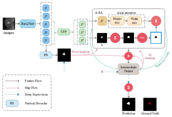
Figure 1.
Overview of the CaPaN. The system contains three contextual modules (the CFP) and the axial reverse attention module (A-RA). “S” stands for the Sigmoid function. Ground truth consists of the tumor regions manually annotated by radiologists—our label data.
This section is divided into two sub-sections: in Section 3.1, the main architecture of the CFP module is presented; and Section 3.2 contains an overall analysis of the CaPaN module. In Section 3.1, we use the CFP to acquire multi-scale feature information. In Section 3.2, we import MRI scans of osteosarcoma patients into the CaPaN, which allows us to determine the position of tumors and perform accurate cutting of smaller objects. The segmentation results can be used as an auxiliary basis for doctors’ clinical diagnoses.
3.1. CFP Module
Feature pyramids (FPs) are widely used in deep learning models for computer vision tasks because of their ability to represent multi-scale features. Since osteosarcomas are characterized by blurred boundaries and indeterminate shapes, the acquisition of more scale features in a single image becomes an important condition for the accurate segmentation of osteosarcomas. The CFP is employed in this model to reduce the number of parameters and the model’s size while still obtaining multi-scale characteristics. In this section, we will go over the fundamentals of the CFP module, such as the functional pyramid channel. The construction of the CFP module is then explained.
3.1.1. Feature Pyramid Channel
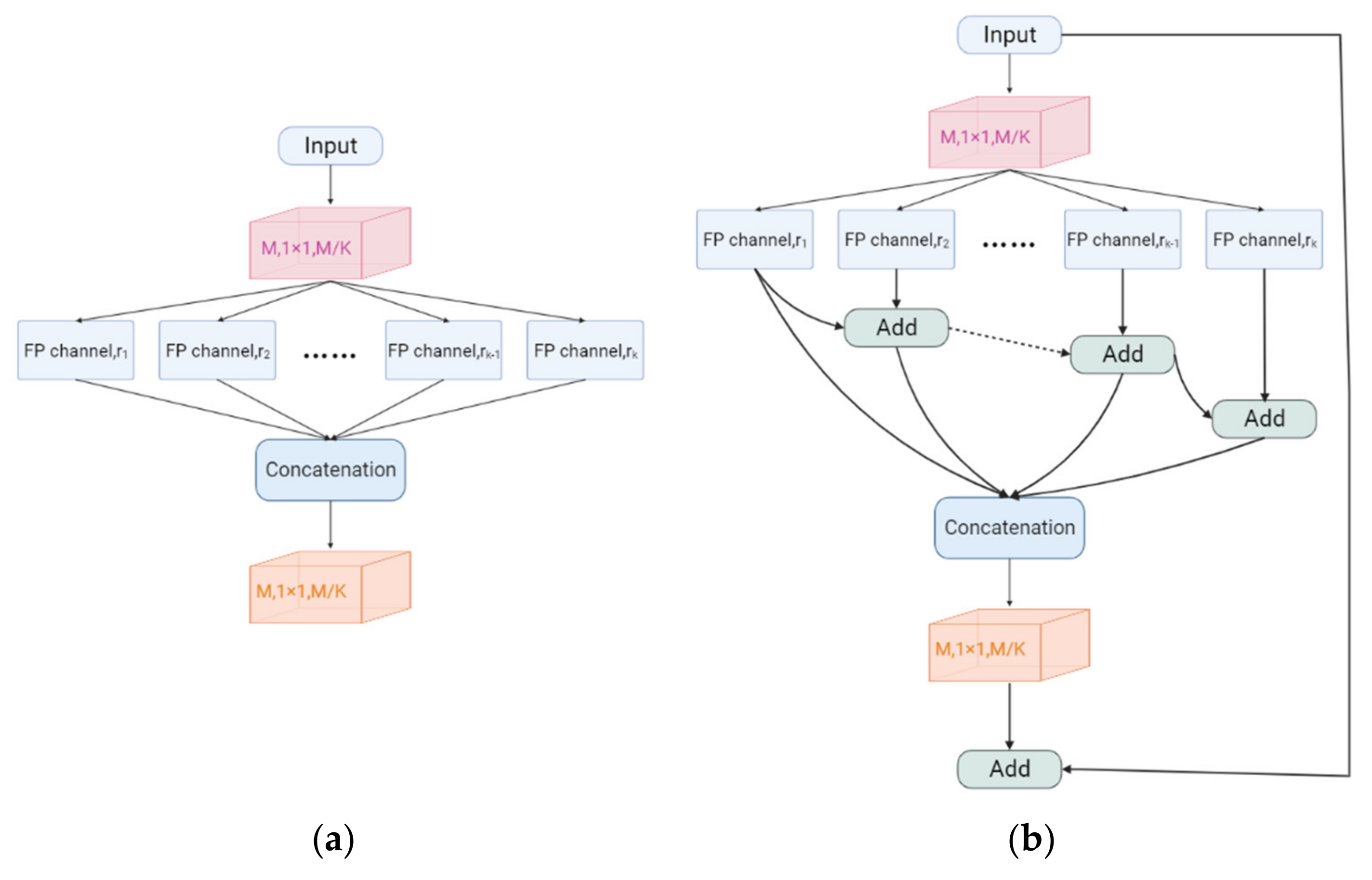
The Feature Pyramid channel is a decomposed form of convolution operator, as shown in Figure 2a,b, which decomposes the convolution of larger kernels into the convolution of smaller kernels. To reduce the resource burden and increase the speed of segmentation, we utilize the FP to decrease the number of parameters while maintaining processing accuracy and ensuring the acquisition of enough features. For the FP channel, we provide two versions of regular convolution and asymmetric convolution, as shown in Figure 2c,d. To avoid too large kernels and too many parameters, we combine the convolution kernels into a channel containing only 3 × 3 kernels. Then, as shown in Figure 2c, we decompose the normal convolution into an asymmetric form to create a feature pyramid (FP) channel. To create multi-scale feature maps, we use jump joints to connect the features extracted from each asymmetric convolution block, allowing each channel to be considered as a sub-pyramid. We choose regular convolution as the FP channel for the CaPaN. These sub-pyramids are connected by a hierarchical feature fusion operation to obtain the overall FP. As shown in Figure 3, the final FP contains four levels of feature stacks :
We calculate the final FP by
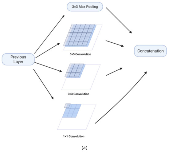

Figure 2.
(a) Naïve inception module. (b) Inception-v2. (c) FP channel with regular convolution. (d) FP channel with asymmetric convolution.
Figure 2.
(a) Naïve inception module. (b) Inception-v2. (c) FP channel with regular convolution. (d) FP channel with asymmetric convolution.

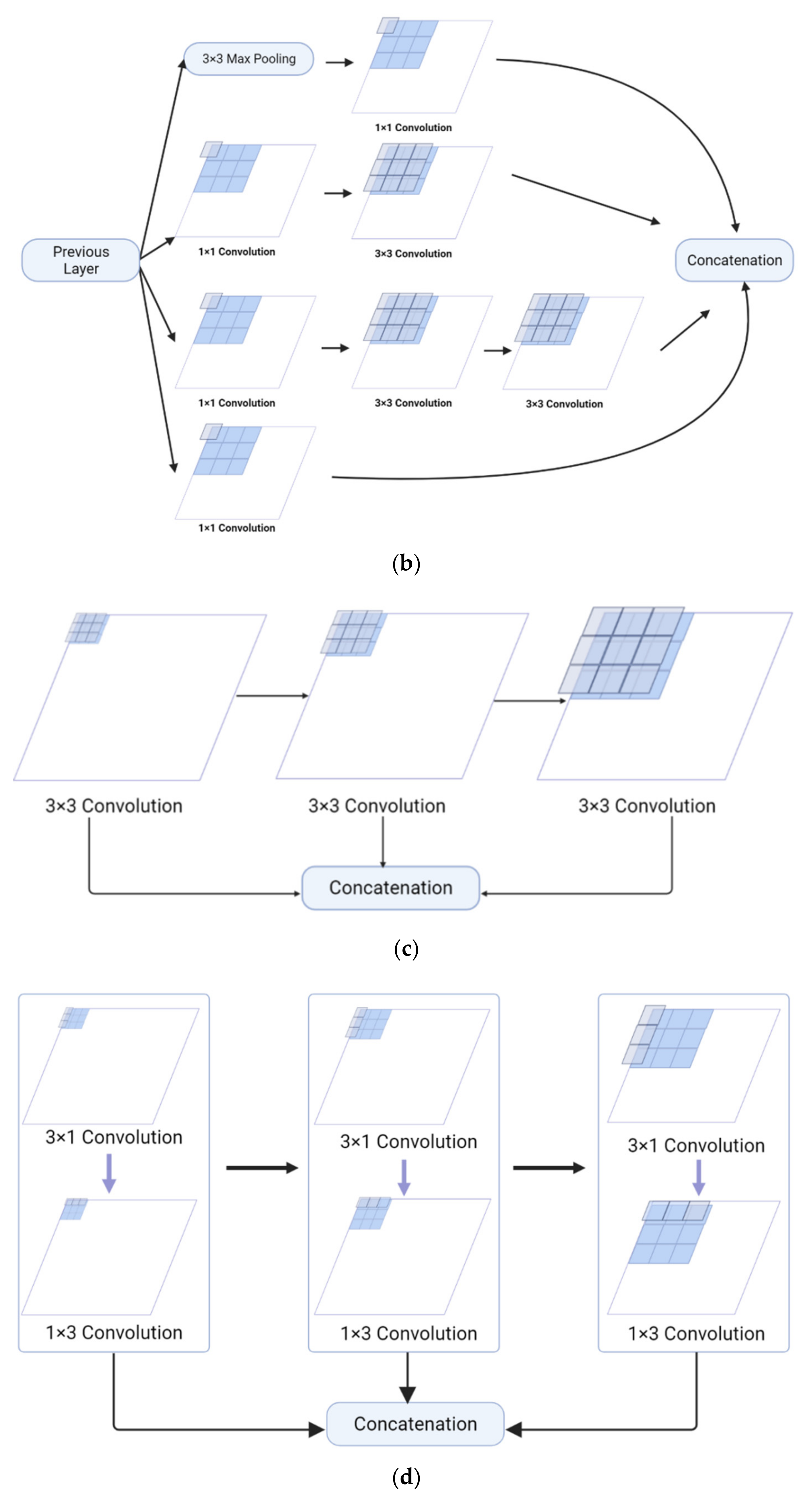
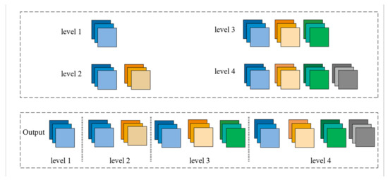
Figure 3.
The final feature pyramid obtained from the CFP module.
Figure 3.
The final feature pyramid obtained from the CFP module.

Compared to the Inception-v2 implementation, the FP channel saves 67% of parameters and reduces the computational resource consumption of the system. However, we can still learn feature information from receptive fields of the same size, allowing us to obtain the same quality of data with fewer resources. We must maintain the same dimensionality of the input and output due to the cascading nature of each asymmetric convolutional block by reordering the number of filters for each asymmetric convolutional block.
3.1.2. CFP Module Structure
We use the CFP module to obtain multi-scale feature information, which allows the network to capture small targets more sensitively. The CFP module can perform calculations accurately and quickly when few parameters have been obtained, which effectively improves the segmentation speed of the model. This is used as an auxiliary basis for clinical diagnosis, and doctors can receive the processing results of the model quickly, which greatly reduces the ineffective waiting time. K FP channels with varying expansion rates {r1, r2, …, rK} are included in the CFP module. To decrease the input dimension from M to M/K, the basic CFP module employs 1 × 1 convolutions. The first to third asymmetric blocks’ dimensions are M/4K, M/4K, and M/2K, respectively.
More information regarding the CFP module may be found in Figure 4. To translate high-dimensional characteristics into low-dimensional features, we employ 1 × 1 convolutions. Different dilution rates are used to set up several FP channels as parallel structures. Then we link all feature mappings to the input dimension and activate the result using another 1 × 1 convolution. As illustrated in Figure 4a, this is the basic structure of the original CFP module. The asymmetric convolution, on the other hand, increases the network’s depth, making training more challenging.
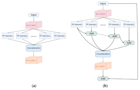
Figure 4.
(a) Original CFP module. (b) CFP module.
Furthermore, a basic fusion approach creates undesirable checkerboard or grid artifacts which have a significant impact on the segmentation mask’s accuracy and quality. In medical tasks, clear medical impact images are important for doctors to quickly analyze conditions. When analyzed manually, artifacts in an image can have an impact on the doctor’s analysis. However, for machines that learn everything from the input for analysis, the impact of artifacts can be even worse. Artifacts can make a machine acquire unnecessary feature information which can affect processing results, and MRI imaging itself is sensitive to magnetic field inhomogeneities and therefore prone to unwanted artifacts. Furthermore, poor magnetic field inhomogeneity at the air–tissue interface can result in substantial sensitivity to artifacts [16], with a greater magnetic field intensity resulting in more severe abnormalities. The segmentation of small objects is the acquisition of fewer features. When the machine acquires unnecessary features, the segmentation results may be more harmful. Therefore, we use residual connections to provide more feature information to remove artifacts produced by this training process, resulting in better segmentation results. We use hierarchical feature fusion (HFF) [36] to alleviate the influence of grid artifacts in the de-grid. The summing procedure is used to progressively integrate the feature maps, starting with the second channel, and then stitch them together into the final hierarchical feature map. Finally, the impact of MRI grid artifacts is decreased, allowing the following models to more precisely capture image characteristics. Figure 4b depicts the final version of the CFP module.
3.2. CaPaN Basic Structure
The architecture of the CaPaN is described in detail in this section. The system generates high-level semantic global maps using a parallel partial decoder [37] and detects global and local feature information using a variety of contextual and axial inverse attention procedures. In this way, it solves the problem of better delineation of osteosarcoma lesion regions in MRI imaging while capturing and segmenting small targets more precisely to improve the accuracy of treatment by physicians and achieve tumor detection at the early stages of tumor growth, enabling better treatment for patients. This section details the architecture of the CaPaN. It uses a parallel partial decoder [37] to generate a high-level semantic global graph and uses various contextual and axial reverse attention operations to detect global and local feature information. Therefore, the CaPaN solves the problem of better delineation of the osteosarcoma lesion area in MRI imaging and can more accurately capture and segment small targets. The segmentation accuracy of CaPaN is high and the results are used as an auxiliary basis for doctors’ diagnoses and treatments which can not only provide doctors with a more accurate reference, but also reduce the time and labor costs required for doctors to double-check the detection. We will introduce the components of this network in the following subsections.
- Parallel Partial Decoder:
Currently, the most popular segmentation models are based on U-Net, which aggregates all levels of the encoder’s feature maps. Most of these segmentation models cannot achieve accurate segmentation of small targets. U-Net using a simple jump-connection scheme is also still a challenge for modeling global multi-scale problems as not every jump-connection setting is effective due to incompatible codec stage feature sets and some jump connections can negatively affect segmentation performance. The U-Net without skip connections performs worse, but the original U-Net performs worse segmentation on some datasets. The proposers of the U-Net++ model, Zhou and Zongwei [38], also stated in their paper that for the feature extraction phase, the downsampling process performed by U-Net returns only after four layers. However, the importance of features at different levels is different for different datasets, and the four-layer U-Net structure cannot guarantee that it is optimal for the segmentation problem of all datasets. Based on the characteristics of large changes in the shape of osteosarcomas and blurred boundaries, the system can accurately segment small osteosarcomas, not only providing good auxiliary support for radiologists’ diagnoses and treatments, but also improving the efficiency of the manual division of lesion areas. This reduces the time and personnel cost of repeated inspections by doctors to ensure the accuracy of the test.
Experiments have shown that low-level features are more computationally intensive but contribute less to improving segmentation performance. Therefore, we combined high-level features using the parallel partial decoder illustrated in Figure 5 to increase segmentation accuracy for the improved acquisition of smaller objects. To extract low-level and high-level characteristics, we used Res2Net [31] as the backbone network. With this, we can retrieve five different levels of features {fi, i = 1, …, 5} with a resolution which is formulated as by feeding the original picture of size h × w × c (h, w, c signify height, width, and channel, respectively) into Res2Net. To aggregate the high-level features, we used the partial decoder PD (∙). To generate the global map Sg, partial decoding features were extracted using PD = pd (f3, f4, f5).
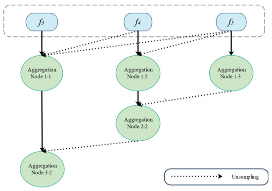
Figure 5.
Overview of the partial parallel decoder.
- Context Module:
Due to the limited annotation available for osteosarcomas, the obtainment of more valid information from the limited information already obtained becomes a critical issue. To obtain contextual information from high-level features, we applied a channel-based feature pyramid (CFP) module to obtain multi-scale feature information to achieve target refinement and to lay the foundation for identifying and segmenting small targets. We set the CFP dilation rate d = 8, so the dilation rate of each channel is {1, 2, 4, 8}. After the context module, we can obtain the multi-scale high-level features {f3′, f4′, f5′}.
- Axial Reverse Attention:
The axial attention path and the reverse attention path make up the Axial Reverse Attention module. The globe map simply depicts the organization’s basic location and lacks structural specifics [39]. As a result, we use reverse attention to gradually mine the distinct tissue areas by eliminating foreground items. While acquiring structural details, the prerequisites for the enhanced acquisition of small targets are met. For the segmentation of osteosarcomas in MRI scans, more comprehensive information is gathered. The inverse operation is written as:
For the other route, we use axial attention to maintain global connectivity and efficient computation [9], allowing improved accuracy while effectively simulating the original self-attentive mechanism for better capture of small targets of osteosarcomas. In axial attention, by computing the horizontal and vertical axes, the network can extract global dependencies and local representations. The output of the A-RA module can be expressed as:
is based on the multiplication of elements, while is a feature of the axial attention path.
- Axial Reverse Attention:
Since osteosarcoma MRI imaging has disadvantages, such as fewer available annotations, we weighted each feature for calculation. A weighted intersection set (IOU) and weighted binary cross-entropy (BCE) are used as loss functions for calculating global loss and local loss that is pixel-level so that a single characteristic does not have too much of an impact on the loss numbers. The stability and accuracy of the learning process are guaranteed. This lays the foundation for acquiring more and more accurate features for osteosarcoma MRI imaging [40]. To prevent the overfitting problem, it is necessary to make sure that the model does not learn in the direction of a certain feature. The loss function may be written as follows:
is calculated as:
where k, kernel_size, is the pooling kernel size; Ni is the batch size of the input ground truth, which is the size of the osteosarcoma MRI image; Cj denotes the number of channels in the input ground-truth signal; s, stride, is the step size of the pooling layer; and m is the ground truth, which is the osteosarcoma region.
is calculated as:
Here, p is the output of the linear layer and does not need to go through the sigmoid layer; m is the ground truth.
denoted as:
where inter is the overlap between the systematically divided tumor area and the correct lesion area. It is calculated as follows:
union, the area of the demarcated osteosarcoma region and the area of the accurate osteosarcoma region added together, uses the formula to compute:
The output of the linear layer after being processed by the sigmoid function is p.
To train the CaPaN, we perform deep supervision on the three sub outputs (, , ) and the global mapping . We upsample the losses to the same magnitude as the ground truth before computing them. As a result, the total loss may be written as:
- Small Object Segmentation Analysis:
The size of an object is defined by the number of pixels in the object (m) and the number of total pixels in the picture (N) since the size of all images submitted to the segmentation model must be fixed. As a result, we use the size ratio (scale) = m/N to consider the object’s size. Then, the performance of the segmentation model is assessed depending on the size of the item. We are particularly interested in smaller regions with area ratios less than 5%.
For the segmentation model, we first obtain the average dice coefficients and size ratios for the segmentation from the test dataset. Similar to computing a histogram, we plot the results on a curve whose y-axis is the average dice coefficient and whose x-axis is the progressively ordered size ratio. To smooth the curve, we take the interval-averaged average dice coefficients by sorting according to size ratio: we divide the entire range of size ratios into a continuous, non-overlapping sequence of equal-length intervals and then calculate the average dice coefficient for each interval’s size ratio. The interval-averaged coefficients have smooth curves and are more stable in the presence of noise. This demonstrates the robustness of our model when segmenting osteosarcoma MRI imaging and the segmentation of small targets is not affected by noise. In this way, the effect of MRI imaging results on the segmentation effect due to the variable performance of medical instruments obtained in developing countries is also addressed.
This study adopts a novel attention-based deep neural network, Res2Net, as the backbone network to obtain multi-scale representations of features. It solves the problem of blurred image features caused by increased signals in MRI imaging of osteosarcomas, thinning, interruption or loss of bone cortex, and soft tissue mass. To overcome the difficulty to balancing local and global features and to better collect tumor feature information in osteosarcoma MRI imaging, a parallel partial decoder is utilized to aggregate advanced features. The CFP module is used as a contextual module to acquire multi-scale feature information. By applying reverse attention to progressively mine the differentiated tissue regions by erasing foreground objects, the inability to accurately capture osteosarcoma features due to the development of the disease and the appearance of other interfering features in MRI imaging is avoided. For the other path, we use axial attention to maintain global connectivity and efficient computation [9]. The redundant computation problem of CNN-based methods is solved, and the waste of resources is reduced. The above features ensure that our model has a good generalization ability and that it solves the generalization problem in practical applications and clinical-level validations. The learning process is not disturbed by image quality and has low data requirements. It makes the application cost of the model low and facilitates expansion in developing countries. Automated and accurate tumor delineation eliminates the personnel and time costs incurred in the manual delineation of tumor areas and avoids the influence of subjective consciousness and the irresistible environmental factors that can accompany manual delineation. It reduces the workload of doctors and provides doctors with better and more accurate auxiliary diagnoses and treatment bases. For patients, more accurate tumor area delineation and small target capture can avoid the stress of follow-up treatments caused by incomplete tumor excision and repeated chemotherapy, which can cause great stress, reducing treatment costs and benefitting the patient’s body and mind.
4. Experimental Results
4.1. Datasets
The Department of Mobile Health Information, Ministry of Education—China Mobile Joint Laboratory, and the Second Xiangya Hospital, Central South University, contributed the data for this work [23]. In addition, we gathered more than 80,000 MRI osteosarcoma pictures and other metrics data from 204 osteosarcoma patients. We placed each picture into the network segmentation system after making image changes, such as rotation, highlighting, flipping, color-changing, and zooming in and out, to acquire the final segmentation results and to make the model segmentation results more accurate and robust. After dataset enhancement, the total training dataset was 4~6 times that of the original dataset, which assists the feature learning and training of the model. In the training process, we first divided the dataset into four subcategories according to disease region, as shown in Figure 6: single leg lateral MRI imaging with tumor present in the leg; single-leg knee lateral MRI imaging with a tumor present in the knee; thigh transverse section MRI imaging with a tumor present in the section; and double leg frontal MRI imaging with a tumor present in one of the legs. Eighty percent of the images in each category were used for training and 20% for testing. After the first round of training, we classified the data with unsatisfactory segmentation results in each class again according to the degree of similarity for the second round of training. Finally, 204 patients with osteosarcoma MRI imaging were classified into six categories to obtain the data used in this study.
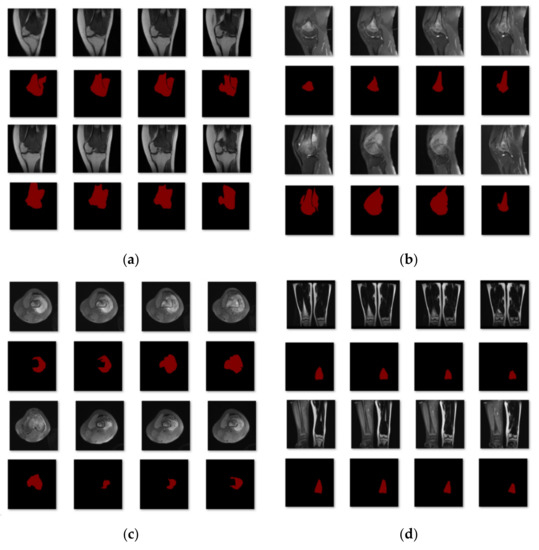
Figure 6.
The first classification results. (a) Class 1: Single leg lateral MRI imaging with a tumor present in the leg. (b) Class 2: Single leg lateral MRI imaging of the knee with a tumor present in the knee. (c) Class 3: MRI imaging of the thigh in the transverse section with a tumor in the section. (d) Class 4: Frontal MRI imaging of both legs with a tumor in one of the legs.
4.2. Training Strategies
CaPaN models require large amounts of data to train. Therefore, the dataset must be enhanced before training to improve the model’s resilience. We extended the dataset by rotating and flipping the images or increasing their brightness. In the training process, the optimizer is ADAM, the initial learning rate is 1 × 10⁻⁴, the decay rate of the learning rate is 0.1, the epoch is 200, each epoch contains 10 batches, and the learning rate is decayed once every 50 epochs.
In the training process, because the CaPaN model requires a certain number of data, we enhanced the dataset by rotating, highlighting, flipping, changing the color, and zooming in or out of images to meet the data volume requirement of the model before training. To begin the training process, we created a class of MRI pictures with the same tumor location (e.g., both leg MRI images) and tumor shapes comparable to those of the ground truth images, then selected 80% for training and the remaining 20% for validation. After the performance of one segmentation procedure, unsatisfactory segmentation results were then separated out for secondary classification and the experiments and classification operations were repeated until satisfactory results were obtained.
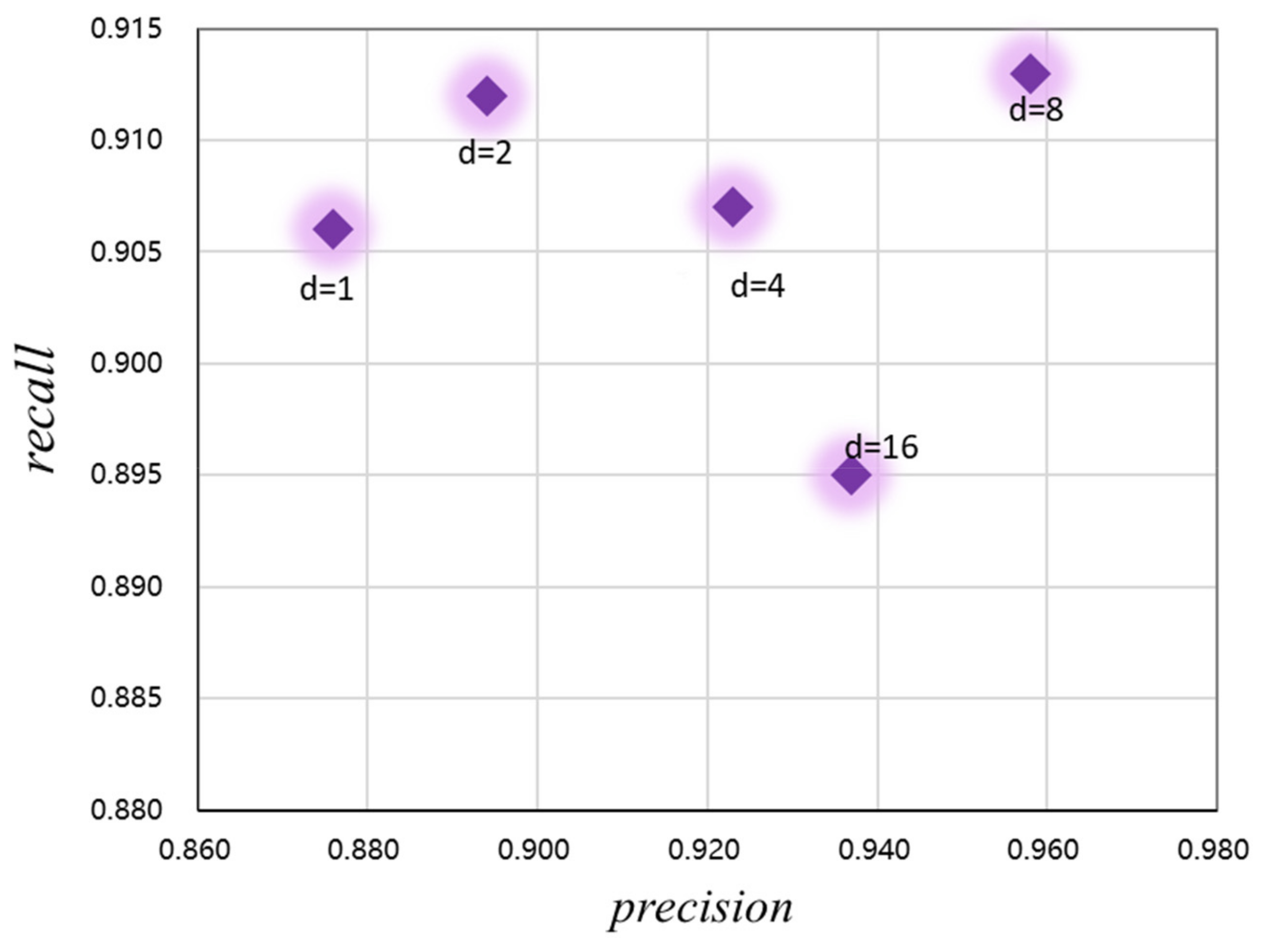
In addition, to optimize the performance of the CaPaN model and better obtain contextual information from the MRI images, we analyzed the expansion rate of the channel-based feature pyramid (CFP), namely, the hyper-parameter, to achieve the refinement of target lesions. By changing the size of the dilated convolution, the receptive field of the model output can be changed. As shown in Figure 7, both the precision and recall of the CaPaN model changes as the dilation rate changes. When the expansion rate is less than or equal to 2, although the recall value is higher, the precision value is lower. When the expansion rate is greater than 8, the recall rate of the CaPaN is higher. When the expansion rate d = 8, the performance of the CaPaN is optimal, and the CFP can better obtain multi-scale information at this time. Therefore, this study set d = 8 for the experimental analysis.
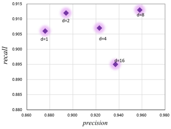
Figure 7.
Relationship between the CaPaN model’s performance and hyper-parameters.
4.3. Algorithm Comparison
We compared the CaPaN with eight of the most common image segmentation methods: FCN [41], FPN [42], MSFCN [43], PSPNet [44], U-Net [45], MSRN [46], SVseg [47], and Ga-CNN [48].
Fully Convolutional Network (FCN): The network employs a jump structure to perform precise segmentation and classifies pictures at the pixel level [41]. The fully connected network is replaced by a convolutional network, which solves the problem of image segmentation at the semantic level. The FCN-16S network that performs 16 upsampling is chosen in this paper.
Pyramid Scene Parsing Network (PSPNet): At the network’s heart is the pyramid pooling module, which collects contextual information from several locations to produce good outcomes in acquiring global information [44]. It can effectively obtain global contextual information for pixel-level scene annotation and the pyramid pooling module it employs has better feature representation capabilities than global pooling.
MSFCN: This model consists of a multi-supervised output layer complete convolutional network for automated tumor segmentation [43]. Its complete convolutional network has supervised side output layers that allow it to collect both global and local picture characteristics. In the upsampling phase, several feature channels are employed to collect more contextual information, ensuring precise tumor segmentation and low contrast of surrounding soft tissues. The final tumor borders are determined by fusing the findings of all side outputs [43].
Multi-scale Residual Network (MSRN): Using residual binning, convolution kernels of various sizes are added to adaptively identify picture characteristics at various scales [46]. The MSRN employs MSRBs to capture visual features at multiple scales and integrates the output of each MSRB for global feature fusion. The utilization of LR image features is maximized by combining local multi-scale features with global features.
U-Net: The U-shaped structure of this network was proposed to tackle the challenge of medical picture segmentation. The network employs convolution for encoding followed by upsampling for decoding [45]. It consists of two parts—feature extraction and higher-layer adoption. It is one of the most often used and simplest segmentation models. U-net is a basic, efficient, easy-to-understand, and simple-to-build neural network that can be trained using tiny datasets.
Feature Pyramid Network (FPN): This network is a feature extractor that aims to boost speed and accuracy. It creates higher-quality feature graph pyramids by replacing the feature extractor in detectors. By merging these distinct levels of features, both the high resolution of the lower-level features and the high semantic information of the higher-level features are used to accomplish prediction [42].
SVseg: This is an automatic segmentation method for vertebral CT images which is mainly based on the Stacked Sparse Autoencoder (SSAE). SVseg includes SSAE and sigmoid classifiers. Among them, SSAE learns raw features from CT images. Sigmoid completes patch classification based on class probabilities [47].
Ga-CNN: A liver CT image segmentation model, which is mainly a lightweight convolutional neural network composed of three convolutional layers and two fully connected layers [48].
4.4. Evaluation Indicators
To better assess the model’s efficacy in segmenting osteosarcomas, as an assessment criterion, we employed the following indexes, as given in Table 1.

Table 1.
Evaluation indexes and corresponding descriptions of the experiment.
First, four terms are clarified: true positive (tp) denotes an instance that belongs to a positive class and is predicted to belong to a positive class, also known as a true class; false positive (fp), also known as false detection, denotes an instance that belongs to a negative class but is predicted to belong to a positive class, also known as a false-positive class; true negative (tn) denotes a positive class that is projected to be a negative class, also known as a true negative class; false negative (fn) denotes a positive class that is predicted to be a negative class, also known as a false-negative class.
IoU (Intersection over Union) is a basic metric for determining the accuracy of finding an item corresponding to a given item in a given dataset [52]. It may be used for any task that produces bounding boxes as a result. The correlation between real and expected values is measured using this criterion; the stronger the correlation, the higher the value. The result of dividing the overlapping portion of two parts by the pooled part of the two regions yields the IoU, which is then compared against the result of this IoU computation using a defined threshold. The following is the formula for calculating it:
The Dice Similarity Coefficient (DSC) is the most commonly used evaluation criterion in the segmentation process [53]. The dice coefficient is a type of set similarity measure, usually used to measure the correlation of two samples with a value range of [0, 1], with the best segmentation results when the value is 1 and the worst when the value is 0. It is defined as follows:
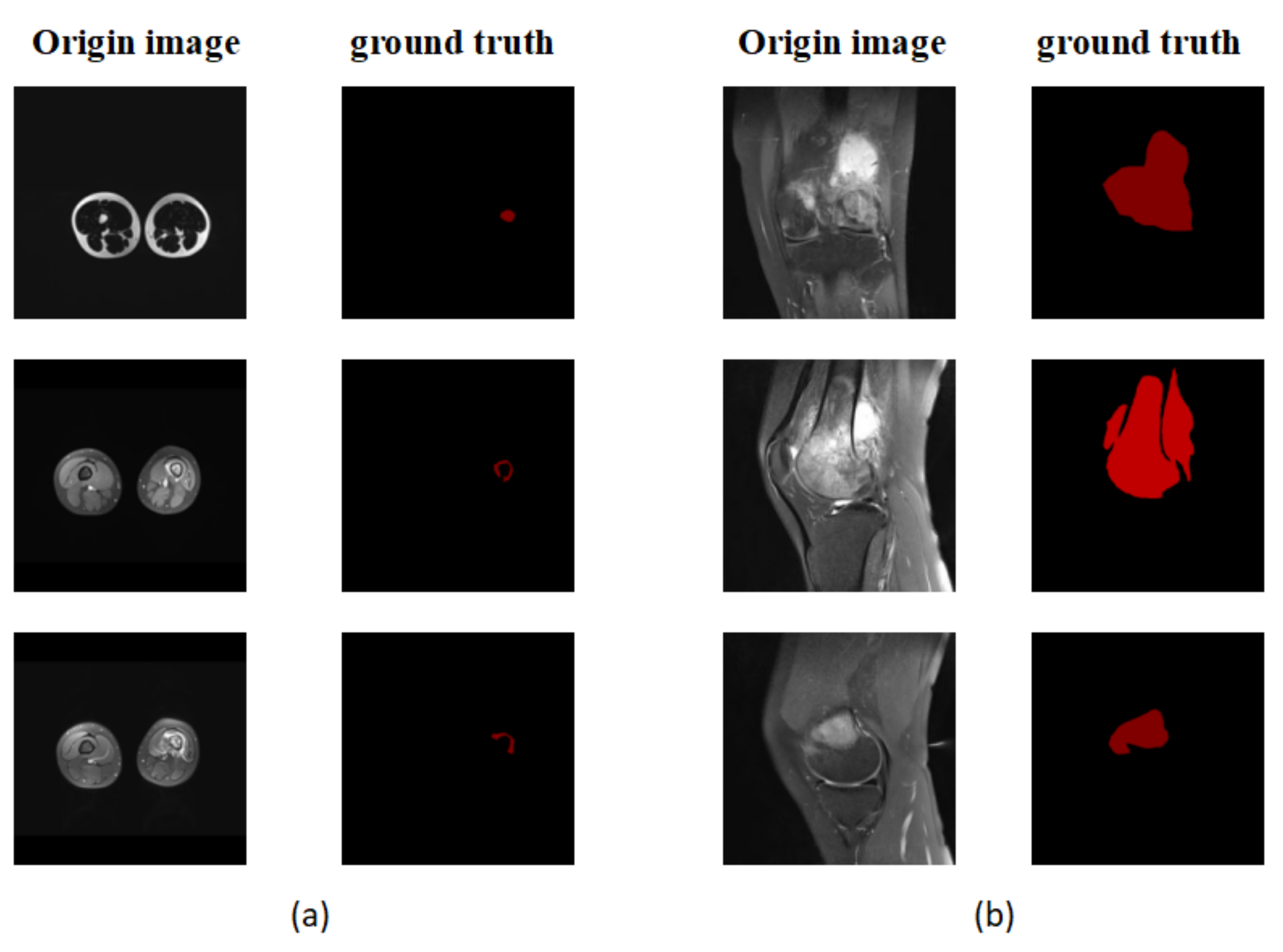
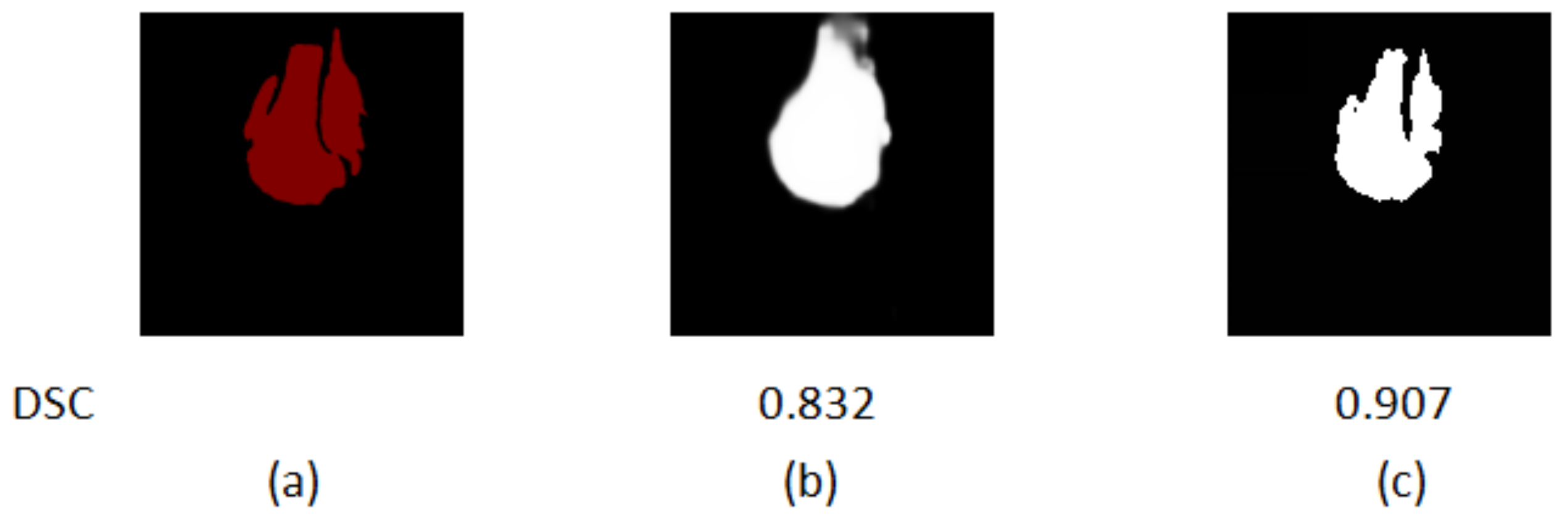
P is the result predicted by the model and G is the picture manually labeled by the doctor. Since the size of all pictures submitted to the segmentation model must be fixed, the size of the object is defined by the number of pixels in the object and the size of the entire image [54]. To determine the size of an item, we utilize the ratio (proportion) of the number of pixels in the object to the total number of pixels in the picture. The segmentation model’s performance is then assessed in relation to the object’s size. We pay special attention to smaller regions, those with a ratio of less than 5%, as shown in Figure 8.
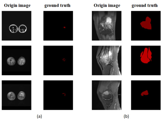
Figure 8.
(a) An example of a small area focused on in the experiment. (b) A non-small area.
4.5. Results
Figure 9 shows a comparison of the model segmentation effects before and after the dataset improvement. The left column represents the ground truth, the center column shows the segmentation result graph of the model before the enhancement of the dataset, and the right column shows the segmentation result of the model after the optimization. When the MRI image was not optimized, the results of the model segmentation shoed fuzzy segmentation and wrong segmentation. The optimized results were closer to the true labels and the completeness and accuracy of the model’s predictions were improved. The model’s performance was greatly enhanced as a result of dataset tuning. We performed a quantitative analysis, shown in Table 2. For the dataset without enhanced processing, the DSC value of the system was only 0.467, the F1 value was only 0.341, and the MAE value reached 0.018. After the dataset was enhanced four times and six times, various indicators were significantly improved, especially after six enhancements. The DCS value increased by 93%, the F1 value increased by 161.58%, and the MAE decreased by 61.2%.
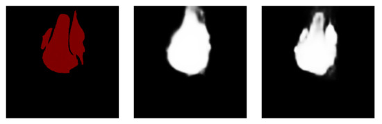
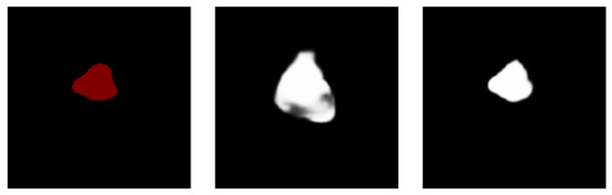
Figure 9.
Before and after the dataset was upgraded: a comparison of the model segmentation effect was made.
Table 2.
Variation in training model performance with four enhancements and six enhancements vs. no enhancements for the overall dataset.
In addition to the dataset enhancement, we also classified different kinds of images in the dataset and then performed training for them separately to improve the segmentation results. The results after different classifications are shown in Figure 10.

Figure 10.
Comparison of the segmentation results of the first classification and the final classification of data in the dataset. (a) The ground truth. (b) The first classification segmentation result. (c) The final result.
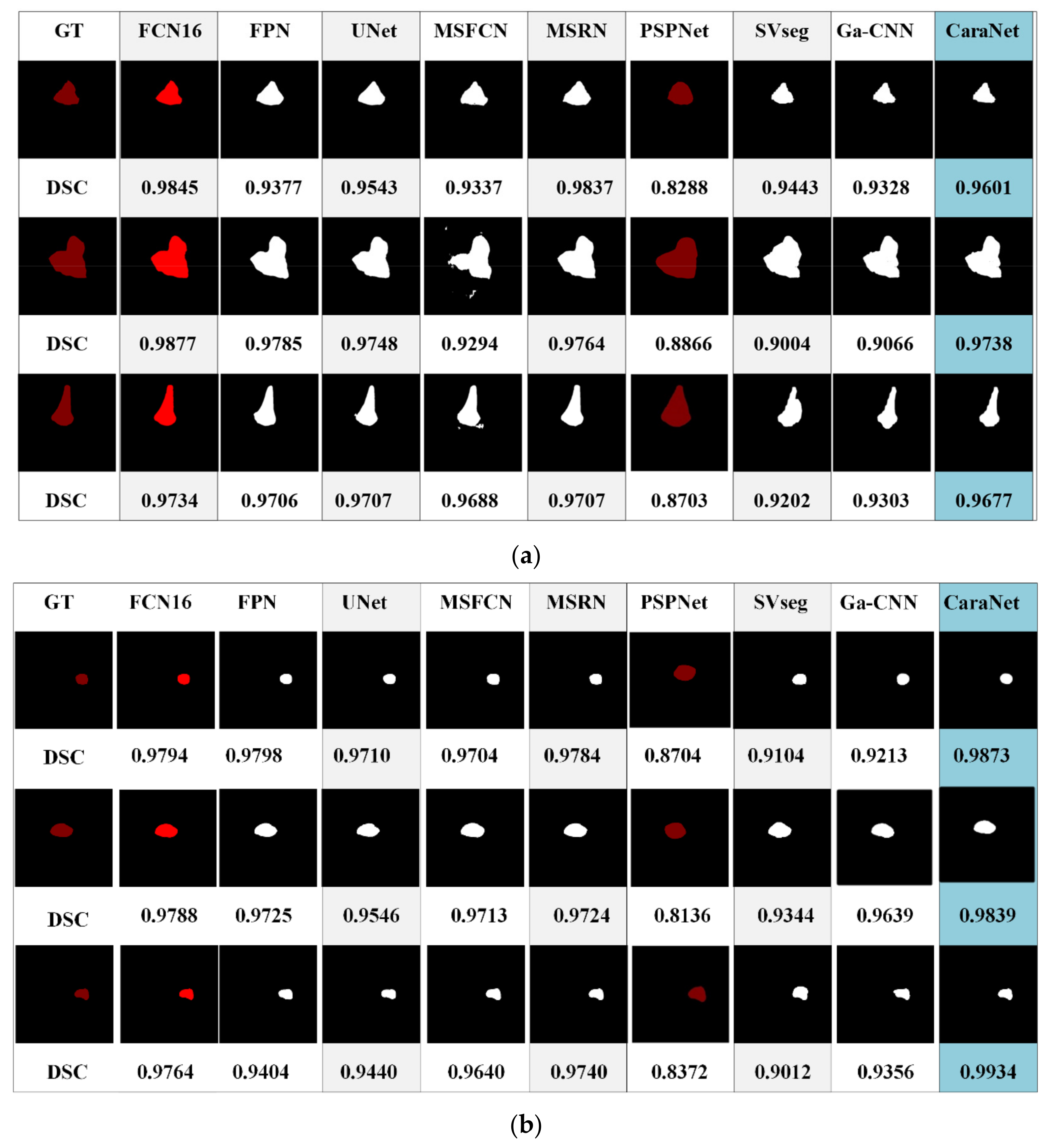
Figure 11 shows the segmentation results of different models for osteosarcoma MRI images. From Figure 11a, it can be seen that the CaPaN can outperform most models in the segmentation of large objects; the DSC value is above the average of the other eight models. It is more accurate in terms of tumor localization and reflecting the nuances of tumor boundaries, without under-segmentation or over-segmentation. When the MSFCN network divides a tumor area, the localization of the lesions is not accurate enough. Both PSPNet and SVseg models suffer from significant over-segmentation. The Ga-CNN network has insufficient segmentation. At the same time, for the segmentation of small objects, the segmentation results of the CaPaN model are also better than those of other models. Its DSC value exceeds that of other models by more than 0.01. The FPN, U-Net, MSFCN, MSRN, PSPNet, and SVseg models all suffer from over-segmentation. In particular, the PSPNet model is not accurate enough to be used to locate small lesions. Compared with these models, Ga-CNN has a better effect but its division of edge parts is still not accurate enough.
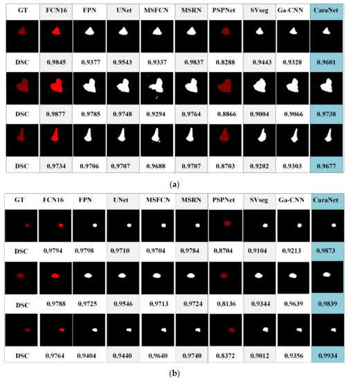
Figure 11.
Different segmentation methods’ effects on segmentation are compared. (a) Small target segmentation vs. non-small target segmentation. (b) Small target segmentation vs. non-small target segmentation.
In order to conduct a clearer comparative analysis of the evaluation indicators, we quantified the segmentation results of different models for small target objects. Table 3 compares the performance of different methods on the small target osteosarcoma dataset. Compared with other models, the CaPaN model has more significant advantages than other models in terms of Pr, IOU, and F1 values. Specifically, the Pr value of the CaPaN model is 0.014 times higher than the accuracy of the second-ranked FCN16 and U-Net models. The F1 and DSC values represented improvements of 0.98% and 2.36%, respectively, in relation to U-Net, and of 3.6% and 6.29% in relation to FCN16. Although the Pr and F1 values of the FPN model are relatively high, its variance is large and the performance of the model is unstable. The variance of the CaPaN model on Pr, F1, and DSC is the smallest, indicating that the data fluctuation of the model is small during the training process, and the CaPaN model has good data stability. In terms of system parameters, the params value of PSPNet is the smallest, but the segmentation accuracy of this model is low. Compared with other models, CaPaN has fewer parameters, indicating that the complexity of the CaPaN model is lower. Although the FLOPs value of CaPaN is slightly higher than that of the MSFCN, MSRN, and U-Net models, the params of CaPaN are much lower than those of the MSFCN and MSRN networks. The segmentation effect and variance of CaPaN are more advantageous than U-Net, and the stability is higher. Overall, the segmentation performance of CaPaN on small target objects outperforms other models in the experiments. In terms of complexity, CaPaN is less complex and has a faster computation rate. It achieves a balance of segmentation accuracy and speed.
Table 3.
Quantitative comparison of MRI performance of patients with osteosarcoma by different methods for small subject segmentation (segmentation target percentage less than 5%).
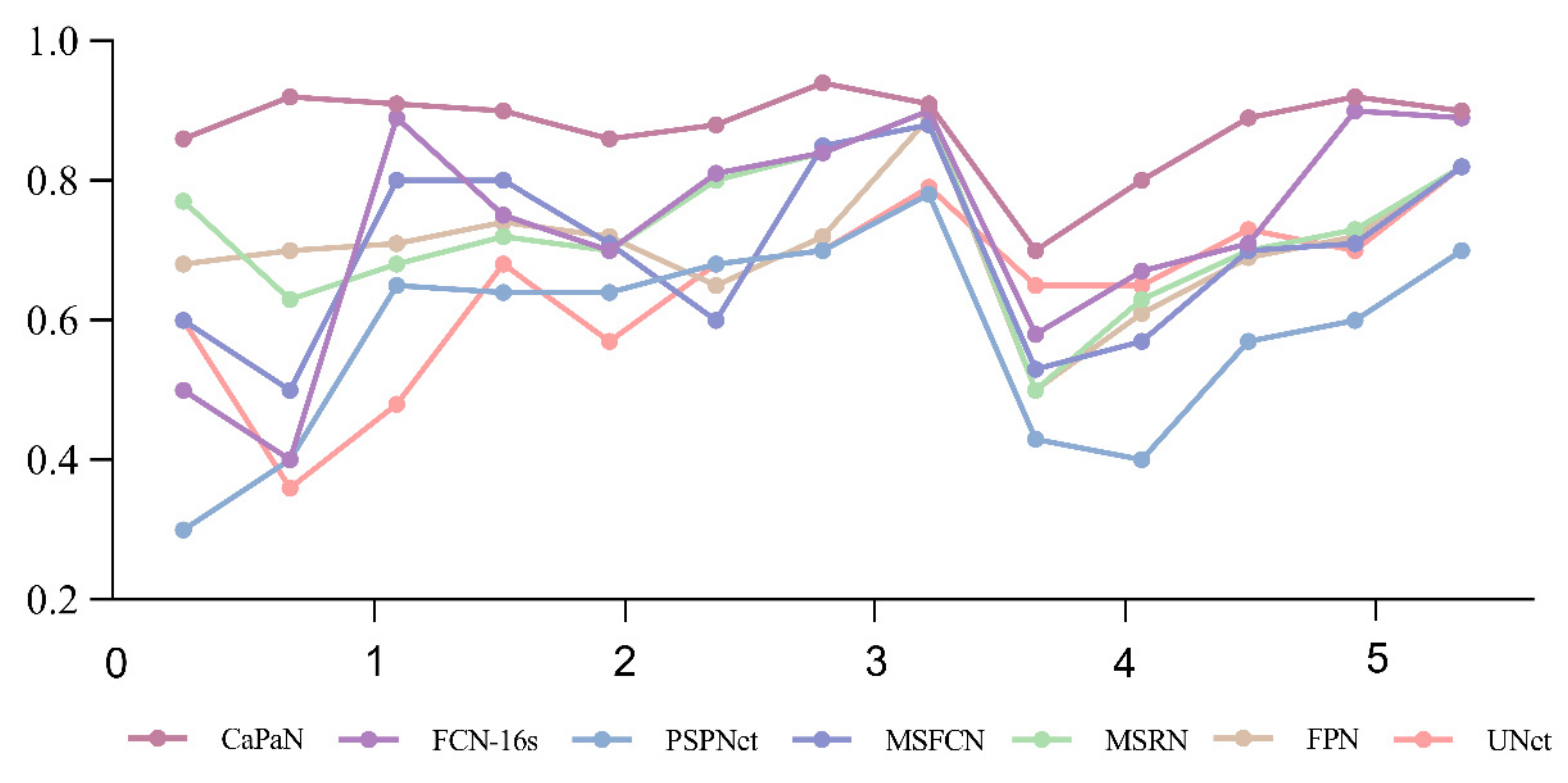
Further, in Figure 12, the DSC values of the segmentation results for small target tumor objects (objects with tumor proportion sizes <5%) are compared for each model. It is easy to see that for the segmentation of small targets, the DSC values of CatraNet’s segmentation results are significantly higher than those of the other models and show good segmentation stability: the difference between the lowest DSC value and the highest DSC for different objects is small and smaller than that of other models.
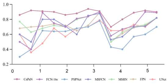
Figure 12.
Comparison of DSC values for the CaPaN with those of different models in small target segmentation. The x-axis represents the proportional size of the tumor (%); the y-axis represents the average dice coefficient.
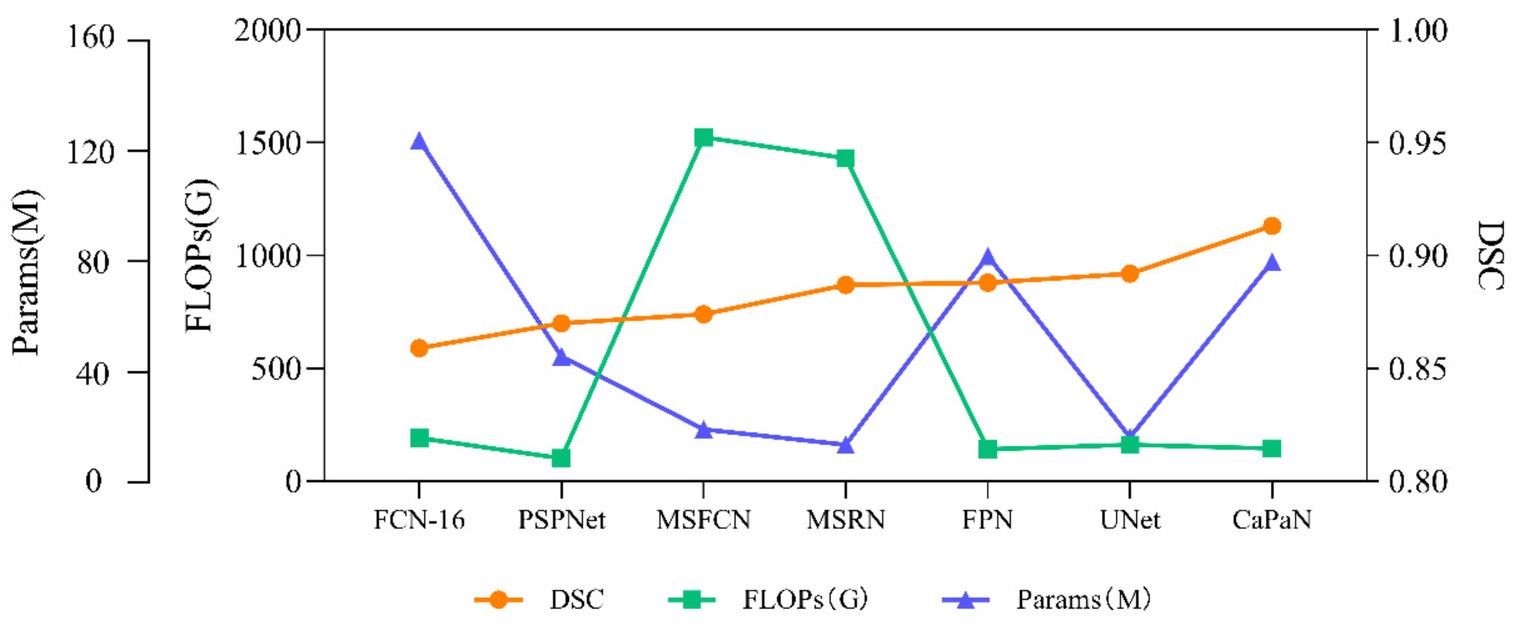
In order to more intuitively compare the relationship between the segmentation performance and complexity of different models for small target objects, we compared the DSC values, params, and FLOPs of the algorithms. It can be seen more intuitively from Figure 13 that CaPaN has a high DSC value without requiring large numbers of parameters and calculations. That is, within an acceptable range, CaPaN can improve segmentation accuracy while avoiding redundancy and heavy computational costs. This means that CaPaN can achieve the desired segmentation results faster and better than other models under the requirement of fast processing of practical large-capacity images.

Figure 13.
Performance comparison of DSC values, params, FLOPs for each model.
Next, we quantified the differences between the various metrics of CaPaN for the overall dataset and the small target dataset. From Table 4, we can see that CaPaN had a good segmentation performance on the whole dataset; it shows better segmentation performance with respect to small target objects than ordinary objects. Although the effect on the overall dataset is worse than that of small target objects, the values of its recall rate, DSC, and other indicators reached more than 0.9. In actual clinical testing, the recall rate is of much greater concern than the accuracy rate. The results show, therefore, that CaPaN is suitable as an auxiliary basis for a doctor’s diagnosis.
Table 4.
Comparison of the segmentation effect of CaPaN on the whole dataset and small target object data (small target object means that the proportion of segmented targets is less than 5%).
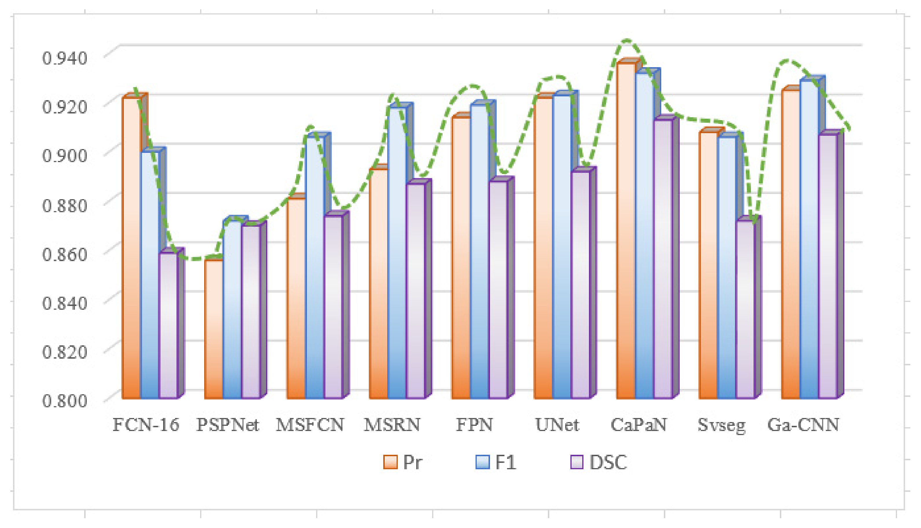
Due to differences in the performance of CaPaN on the overall dataset with small target objects, we compared the segmentation performance of CaPaN with other models on the overall dataset. Figure 11a shows the overall result; Figure 14 shows the overall performance of CaPaN compared to other models for the entire osteosarcoma MRI dataset. The worst segmentation performance was shown by the PSPNet model, whose precision, F1, and DSC values were all below 0.88. The MSFCN network has been significantly improved in all aspects; the precision and F1 values, in particular, have been significantly improved. Although FCN-16 has higher Pr and F1 values, it has the lowest DCS value and is not suitable for the segmentation of osteosarcoma MRI images. Ga-CNN and SVseg outperform other models. The DSC value and F1 value of Ga-CNN are only lower than CaPaN; the DSC value reaches 0.907 and the F1 value reaches 0.929. The indicators for SVseg are relatively low. Although the precision value of SVseg is only 0.908, this is far from those of other models, such as MSFCN and MSRN. Our CaPaN model achieved a value above 0.9, even though the Pr and F1 values are not the highest. The DSC value of CaPaN, however, is the highest, so, in general, the performance of CaPaN is the best. In addition to the results shown in the figure, the structural metric value of CaPaN in the experiment reached 0.942, the average specificity during the test reached 0.924, and the average sensitivity reached 0.934.

Figure 14.
Comparison of CaPaN’s performance with the performances of other models for the whole dataset.
4.6. Discussion
Our proposed Axial-Preserving Attention Network-Based Osteosarcoma Segmentation Model (CaPaN) combines backward attention and a feature pyramid (FP). From the results in Section 4.4, it can be seen that each model has its own advantages. When using the overall dataset for experiments, Ga-CNN and SVseg perform better. When experimenting with a small target object dataset, U-Net’s metrics are high. However, in general, CaPaN shows better performance in the segmentation of osteosarcoma MRI images. Whether facing the overall MRI dataset or the dataset of small targets, the advantages of CaPaN are very significant, especially when it comes to the segmentation of small lesion areas or the subtleties of tumors, the DSC value reaching 0.913. Although there is still a certain gap between this and the lesion area manually marked by radiologists, the segmentation results of CaPaN can be used as an auxiliary basis for doctors’ clinical diagnoses.
Although CaPaN has achieved good segmentation results for MRI images of osteosarcoma, it still faces great challenges in practical environments. On the one hand, CaPaN has many limitations. For example, due to differences in different medical imaging equipment, the brightness of MRI images is not uniform. If our dataset does not undergo data enhancement processing, the segmentation effect is relatively poor. Furthermore, our method is only applicable to 2D images, and there has been no discussion of validating its segmentation performance with respect to 3D images. In actual clinical diagnosis, 3D visualization can provide a more intuitive and comprehensive understanding of tumor information, which is helpful for doctors to judge and analyze a patient’s condition. On the other hand, clinical equipment is determined by medical institutions after multiple selections and comparisons and our model has not been systematically trained. In addition, the complex conditions of different patients, tumors of different scales in the same patient, and different magnetic resonance instruments will lead to differences in the results of the system. Therefore, the model segmentation results can only be used as an auxiliary basis for diagnoses and cannot replace doctors for clinical diagnosis and treatment.
5. Conclusions
The CaPaN segmentation model presented in this study is composed of axial backward attention and channel feature pyramid (CFP) modules. Small medical object segmentation can be improved using this innovative technology. CaPaN effectively improves the segmentation accuracy of small osteosarcoma objects with an appropriate increase in computational power. CaPaN can more accurately identify smaller tumor targets and it can provide a more accurate auxiliary basis for doctors to detect and diagnose disease.
In the future, with the development of artificial intelligence in the medical field and people’s attention to health, we will add dataset enhancement algorithms or use multi-scale training strategies to improve the model. By these means, the workload before training will be reduced and more time and economic costs will be saved for medical auxiliary diagnosis. Furthermore, to address the problem of models relying on prior knowledge, we will continue to investigate the learning of high-level features from unlabeled MRI images in an unsupervised manner.
Author Contributions
Writing—original draft, F.L.; Writing—review & editing, F.G. and J.W. All authors have read and agreed to the published version of the manuscript.
Funding
This work received funding from the Hunan Provincial Natural Science Foundation of China (2018JJ3299, 2018JJ3682) and Focus on Research and Development Projects in Shandong Province (Soft Science Project), no. 2021RKY02029.
Institutional Review Board Statement
Not applicable.
Informed Consent Statement
Not applicable.
Data Availability Statement
Data used to support the findings of this study are currently under embargo while the research findings are commercialized. Requests for data, 12 months after publication of this article, will be considered by the corresponding author.
Conflicts of Interest
The authors declare no conflict of interest.
References
- Eaton, B.R.; Schwarz, R.; Vatner, R.; Yeh, B.; Claude, L.; Indelicato, D.J.; Laack, N. Osteosarcoma. Pediatr. Blood Cancer 2021, 68, e28352. [Google Scholar] [CrossRef] [PubMed]
- Mahore, S.; Bhole, K.; Rathod, S. Comparative analysis of machine learning algorithm for classification of different osteosarcoma types. In Proceedings of the 2021 12th International Conference on Computing Communication and Networking Technologies (ICCCNT), Kharagpur, India, 6–8 July 2021; pp. 1–5. [Google Scholar] [CrossRef]
- Kayal, E.B.; Kandasamy, D.; Yadav, R.; Bakhshi, S.; Sharma, R.; Mehndiratta, A. Automatic segmentation and RECIST score evaluation in osteosarcoma using diffusion MRI: A computer aided system process. Eur. J. Radiol. 2020, 133, 109359. [Google Scholar] [CrossRef] [PubMed]
- Sinha, A.; Dolz, J. Multi-scale self-guided attention for medical image segmentation. IEEE J. Biomed. Health Inform. 2021, 25, 121–130. [Google Scholar] [CrossRef] [PubMed] [Green Version]
- Osadebey, M.; Pedersen, M.; Arnold, D.; Wendel-Mitoraj, K. Image quality evaluation in clinical research: A case study on brain and cardiac MRI images in multi-center clinical trials. IEEE J. Transl. Eng. Health Med. 2018, 6, 1–15. [Google Scholar] [CrossRef] [PubMed]
- Zhou, W.; Yang, Y.; Yu, C.; Liu, J.; Duan, X.; Weng, Z.; Chen, D.; Liang, Q.; Fang, Q.; Zhou, J.; et al. Ensembled deep learning model outperforms human experts in diagnosing biliary atresia from sonographic gallbladder images. Images. Nat. Commun. 2021, 12, 1259. [Google Scholar] [CrossRef]
- Saraf, R.; Datta, A.; Sima, C.; Hua, J.; Lopes, R.; Bittner, M.L.; Miller, T.; Wilson-Robles, H.M. In silico modeling of the induction of apoptosis by Cryptotanshinone in osteosarcoma cell lines. IEEE ACM Trans. Comput. Biol. Bioinform. 2020. [Google Scholar] [CrossRef]
- Tian, X.; Tan, Y. Hospital evaluation mechanism based on mobile health for IoT system in social networks. Comput. Biol. Med. 2019, 109, 138–147. [Google Scholar]
- Cui, R.; Chen, Z.; Tan, Y.; Yu, G. A multiprocessing scheme for pet image pre-screening, noise reduction, segmentation and lesion partitioning. IEEE J. Biomed. Health Inform. 2021, 25, 1699–1711. [Google Scholar] [CrossRef]
- Yu, G.; Wu, J. Efficacy prediction based on attribute and multi-source data collaborative for auxiliary medical system in developing countries. Neural Comput. Applic. 2022, 34, 5497–5512. [Google Scholar] [CrossRef]
- Lou, A.; Guan, S.; Ko, H.; Loew, M. CaPaN: Context Axial reverse attention network for segmentation of small medical objects. arXiv 2021, arXiv:2108.07368. [Google Scholar]
- Chang, L.; Moustafa, N.; Bashir, A.K.; Yu, K. AI-driven synthetic biology for non-small cell lung cancer drug effectiveness-cost analysis in intelligent assisted medical systems. IEEE J. Biomed. Health Inf. 2021, 1–12. [Google Scholar] [CrossRef]
- Zhuang, Q.; Dai, Z. Deep active learning framework for lymph nodes metastases prediction in medical support system. Comput. Intell. Neurosci. 2022, 2022, 4601696. [Google Scholar] [CrossRef]
- Pang, S.; Pang, C.; Zhao, L.; Chen, Y.; Su, Z.; Zhou, Y.; Huang, M.; Yang, W.; Lu, H.; Feng, Q. SpineParseNet: Spine parsing for volumetric MR image by a two-stage segmentation framework with semantic image representation. IEEE Trans. Med. Imaging 2021, 40, 262–273. [Google Scholar] [CrossRef]
- Gou, F.; Wu, J. Triad link prediction method based on the evolutionary analysis with IoT in opportunistic social networks. Comput. Commun. 2022, 181, 143–155. [Google Scholar] [CrossRef]
- Li, L.; Gou, F.; Wu, J. Modified data delivery strategy based on stochastic block model and community detection with IoT in opportunistic social networks. Wirel. Commun. Mob. Comput. 2022, 2022, 5067849. [Google Scholar] [CrossRef]
- Oksuz, I.; Clough, J.R.; Ruijsink, B.; Anton, E.P.; Bustin, A.; Cruz, G.; Prieto, C.; King, A.P.; Schnabel, J.A. Deep learning-based detection and correction of cardiac MR motion artefacts during reconstruction for high-quality segmentation. IEEE Trans. Med. Imaging 2020, 39, 4001–4010. [Google Scholar] [CrossRef]
- Chen, L.; Bentley, P.; Mori, K.; Misawa, K.; Fujiwara, M.; Rueckert, D. DRINet for medical image segmentation. IEEE Trans. Med. Imaging 2018, 37, 2453–2462. [Google Scholar] [CrossRef]
- Gou, F.; Wu, J. Message transmission strategy based on recurrent neural network and attention mechanism in IoT system. J. Circuits Syst. Comput. 2022, 31, 2250126. [Google Scholar] [CrossRef]
- Wu, J.; Xia, J.; Gou, F. Information transmission mode and IoT community reconstruction based on user influence in opportunistic social networks. Peer to Peer Netw. Appl. 2022, 15, 1398–1416. [Google Scholar] [CrossRef]
- Tan, Y.; Wu, J.; Gou, F. A staging auxiliary diagnosis model for non-small cell lung cancer based the on intelligent medical system. Comput. Math. Methods Med. 2021, 2021, 6654946. [Google Scholar] [CrossRef]
- Zhan, X.; Long, H.; Duan, X.; Kong, G. A convolutional neural network-based intelligent medical system with sensors for assistive diagnosis and decision-making in non-small cell lung cancer. Sensors 2021, 21, 7996. [Google Scholar] [CrossRef] [PubMed]
- Yang, S.; Zhou, Z.; Xie, P.; Xu, N.; Dai, Z. Intelligent segmentation medical assistance system for mri images of osteosarcoma in developing countries. Comput. Math. Methods Med. 2022, 2022, 6654946. [Google Scholar] [CrossRef]
- Deng, Y.; Gou, F.; Wu, J. Hybrid data transmission scheme based on source node centrality and community reconstruction in opportunistic social networks. Peer to Peer Netw. 2021, 14, 3460–3472. [Google Scholar] [CrossRef]
- Nasor, M.; Obaid, W. Segmentation of osteosarcoma in MRI images by K-means clustering, Chan-Vese segmentation, and iterative Gaussian filtering. IET Image Process. 2021, 15, 1310–1318. [Google Scholar] [CrossRef]
- Kayal, E.B.; Kandasamy, D.; Sharma, R.; Bakhshi, S.; Mehndiratta, A. Segmentation of osteosarcoma tumor using diffusion weighted MRI: A comparative study using nine segmentation algorithms. Signal Image Video Process. 2020, 14, 727–735. [Google Scholar] [CrossRef]
- Frangi, A.F.; Egmont-Petersen, M.; Niessen, W.J.; Reiber, J.H.C.; Viergever, M.A. Bone tumor segmentation from MR perfusion images with neural networks using multi-scale pharmacokinetic features. Image Vis. Comput. 2001, 19, 679–690. [Google Scholar] [CrossRef]
- Huang, W.-B.; Wen, D.; Yan, Y.; Yuan, M.; Wang, K. Multi-target osteosarcoma MRI recognition with texture context features based on CRF. In Proceedings of the 2016 International Joint Conference on Neural Networks (IJCNN), Vancouver, BC, Canada, 24–29 July 2016; pp. 3978–3983. [Google Scholar] [CrossRef]
- Mandava, R.; Alia, O.M.; Wei, B.C.; Ramachandram, D.; Aziz, M.E.; Shuaib, I.L. Osteosarcoma segmentation in MRI using dynamic Harmony Search based clustering. In Proceedings of the 2010 International Conference of Soft Computing and Pattern Recognition, Cergy-Pontoise, France, 7–10 December 2010; pp. 423–429. [Google Scholar] [CrossRef]
- Huang, W.B.; Wang, Y.J. A New Method for osteosarcoma recognition based on bayesian classifier. Appl. Mech. Mater. 2014, 543–547, 2901. [Google Scholar] [CrossRef]
- Nabid, R.A.; Rahman, M.L.; Hossain, M.F. Classification of osteosarcoma tumor from histological image using sequential RCNN. In Proceedings of the 2020 11th International Conference on Electrical and Computer Engineering (ICECE), Dhaka, Bangladesh, 17–19 December 2020; pp. 363–366. [Google Scholar]
- Hong, F.; Zhao, Y.; Sun, H.; Li, M.; Mei, J. Segmentation of osteosarcoma based on analysis of blood-perfusion EPI series. In Proceedings of the 2004 International Conference on Communications, Circuits and Systems (IEEE Cat. No.04EX914), Chengdu, China, 27–29 June 2004; Volume 2, pp. 955–959. [Google Scholar] [CrossRef]
- Michael, B.; Jaeger, P.F.; Isensee, F.; Maier-Hein, K.H. nnDetection: A self-configuring method for medical object detection. arXiv 2021, arXiv:2106.00817. [Google Scholar] [CrossRef]
- Luo, X.; Song, T.; Wang, G.; Chen, J.; Chen, Y.; Li, K.; Metaxas, D.N.; Zhang, S. SCPM-Net: An anchor-free 3D lung nodule detection network using sphere representation and center points matching. Med. Image Anal. 2022, 75, 102287. [Google Scholar] [CrossRef]
- Peng, H.; Sun, H.; Guo, Y. 3D multi-scale deep convolutional neural networks for pulmonary nodule detection. PLoS ONE 2021, 16, e0244406. [Google Scholar] [CrossRef]
- Gao, H.; Chen, Z.; Li, C. Hierarchical shrinkage multiscale network for hyperspectral image classification with hierarchical feature fusion. IEEE J. Sel. Top. Appl. Earth Obs. Remote Sens. 2021, 14, 5760–5772. [Google Scholar] [CrossRef]
- Wu, J.; Gou, F.; Tian, X. Disease control and prevention in rare plants based on the dominant population selection method in opportunistic social networks. Comput. Intell. Neurosci. 2022, 2022, 1489988. [Google Scholar] [CrossRef]
- Zhou, Z.; Rahman Siddiquee, M.M.; Tajbakhsh, N.; Liang, J. UNet++: A Nested U-Net Architecture for Medical Image Segmentation. In Deep Learning in Medical Image Analysis and Multimodal Learning for Clinical Decision Support: DLMIA ML-CDS 2018 2018; Springer: Berlin/Heidelberg, Germany, 2018; Volume 11045. [Google Scholar] [CrossRef] [Green Version]
- Gao, S.-H.; Cheng, M.-M.; Zhao, K.; Zhang, X.-Y.; Yang, M.-H.; Torr, P. Res2Net: A New Multi-Scale Backbone Architecture. IEEE Trans. Pattern Anal. Mach. Intell. 2021, 43, 652–662. [Google Scholar] [CrossRef] [Green Version]
- Wu, J.; Gou, F.; Xiong, W.; Zhou, X. A Reputation Value-Based Task-Sharing Strategy in Opportunistic Complex Social Networks. Complexity 2021, 2021, 8554351. [Google Scholar] [CrossRef]
- Shelhamer, E.; Long, J.; Darrell, T. Fully convolutional networks for semantic segmentation. IEEE Trans. Pattern Anal. Mach. Intell. 2017, 39, 640–651. [Google Scholar] [CrossRef]
- Lin, T.-Y.; Dollár, P.; Girshick, R.; He, K.; Hariharan, B.; Belongie, S. Feature pyramid networks for object detection. In Proceedings of the 2017 IEEE Conference on Computer Vision and Pattern Recognition (CVPR), Honolulu, HI, USA, 21–26 July 2017; pp. 936–944. [Google Scholar] [CrossRef] [Green Version]
- Huang, L.; Xia, W.; Zhang, B.; Qiu, B.; Gao, X. MSFCN-multiple supervised fully convolutional networks for the osteosarcoma segmentation of CT images. Comput. Methods Progr. Biomed. 2017, 143, 67–74. [Google Scholar] [CrossRef]
- Zhao, H.; Shi, J.; Qi, X.; Wang, X.; Jia, J. Pyramid scene parsing network. In Proceedings of the 2017 IEEE Conference on Computer Vision and Pattern Recognition (CVPR), Honolulu, HI, USA, 21–26 July 2017; pp. 6230–6239. [Google Scholar] [CrossRef] [Green Version]
- Ronneberger, O.; Fischer, P.; Brox, T. U-Net: Convolutional networks for biomedical image segmentation. In Medical Image Computing and Computer-Assisted Intervention—MICCAI 2015. MICCAI 2015; Navab, N., Hornegger, J., Wells, W., Frangi, A., Eds.; Springer: Berlin/Heidelberg, Germany, 2015; Volume 9351. [Google Scholar] [CrossRef] [Green Version]
- Zhang, R.; Huang, L.; Xia, W.; Zhang, B.; Qiu, B.; Gao, X. Multiple supervised residual network for osteosarcoma segmentation in CT images. Comput. Med Imaging Graph. 2018, 63, 1–8. [Google Scholar] [CrossRef]
- Qadri, S.F.; Shen, L.; Ahmad, M.; Qadri, S.; Zareen, S.S.; Akbar, M.A. SVseg: Stacked sparse autoencoder-based patch classification modeling for vertebrae segmentation. Mathematics 2022, 10, 796. [Google Scholar] [CrossRef]
- Ahmad, M.; Qadri, S.F.; Qadri, S.; Saeed, I.A.; Zareen, S.S.; Iqbal, Z.; Alabrah, A.; Alaghbari, H.M.; Rahman, S.M.M. A lightweight convolutional neural network model for liver segmentation in medical diagnosis. Comput. Intell. Neurosci. 2022, 2022, 7954333. [Google Scholar] [CrossRef]
- Shen, Y.; Gou, F.; Dai, Z. Osteosarcoma MRI image-assisted segmentation system based on guided aggregated bilateral network. Mathematics 2022, 10, 1090. [Google Scholar] [CrossRef]
- Chang, L.; Yu, G. Effective data decision-making and transmission system based on mobile health for chronic disease management in the elderly. IEEE Syst. J. 2021, 15, 5537–5548. [Google Scholar] [CrossRef]
- Pang, S.; Feng, Q.; Lu, Z.; Jiang, J.; Zhao, L.; Lin, L.; Li, X.; Lian, T.; Huang, M.; Yang, W. Hippocampus segmentation based on iterative local linear mapping with representative and local structure-preserved feature embedding. IEEE Trans. Med. Imaging 2019, 38, 2271–2280. [Google Scholar] [CrossRef]
- Zhou, X.-Y.; Zheng, J.-Q.; Li, P.; Yang, G.-Z. ACNN: A full resolution dcnn for medical image segmentation. In Proceedings of the 2020 IEEE International Conference on Robotics and Automation (ICRA), Philadelphia, PA, USA, 31 May–31 August 2020; pp. 8455–8461. [Google Scholar] [CrossRef]
- Zhuang, Q.; Tan, Y. Auxiliary medical decision system for prostate cancer based on ensemble method. Comput. Math. Methods Med. 2020, 2020, 6509596. [Google Scholar] [CrossRef]
- Yang, W.; Luo, J.; Wu, J. Application of information transmission control strategy based on incremental community division in IoT platform. IEEE Sensors J. 2021, 21, 21968–21978. [Google Scholar] [CrossRef]


Publisher’s Note: MDPI stays neutral with regard to jurisdictional claims in published maps and institutional affiliations. |
© 2022 by the authors. Licensee MDPI, Basel, Switzerland. This article is an open access article distributed under the terms and conditions of the Creative Commons Attribution (CC BY) license (https://creativecommons.org/licenses/by/4.0/).