1. Introduction
In recent years, many retailers sell their products through not only offline but also online platforms. The sales of perishable goods on e-commerce platforms have experienced a huge growth in China. Compared with the sales in the Spring Festival of 2019, the average daily increases in sales of JingDong Daojia and Dingdong Maicai services in the Spring Festival of 2020 hit 247.84% and 213.50%, respectively. The growths in new users at Duodian and Dingdong Maicai were 298.29% and 291.42%, respectively. In addition, during the Spring Festival of 2020, spanning 24–30 January, the average number of daily active users of perishable goods home delivery retail platforms reached 8.791 million (
http://yuqing.people.com.cn/n1/2020/0318/c209043-31636868.html, accessed on 28 April 2020).
Perishable goods refer to products that are affected by temperature and humidity and are prone to such quality problems as deterioration, decay, or mildew during the storage period. They have the characteristics of being perishable and having short shelf lives. Their residual value is often zero at the end of the sales cycle. Meanwhile, the demands for perishable goods are often uncertain (see [
1]). In [
2], they analyzed the weaknesses of the existing inventory models of perishable products, built the exponential freshness function, and studied the problem of order quantity and shelf distribution combination considering freshness and shelf quantity. In [
3], they studied the impact of the temporary price strategy of perishable products on their sales volumes. In [
4], he empirically investigated the mechanism of selling perishable products. In [
5], they considered a lot size problem for perishable products. In [
6], they studied the inventory policy for a system with substitutable and perishable products. In [
7,
8], they proposed an opaque selling plan for the perishable product system. In [
9], they considered the inventory control and pricing policy for perishable products with social learning. Different from these papers, we explore the impact of overconfidence on the operations of the retailer that sells perishable agricultural products.
Incidentally, there have been many news reports that some perishable products decayed and wasted due to excessive orders. Data from NRDC 2012 and ReFED 2018 show that about 40% of food in the U.S. is dumped straightly into landfills every year, which is equivalent to USD 218 billion in economic losses. U.S. supermarkets and catering industry contribute to 40% of the total food waste, where the supermarket waste is much higher than that of the catering industry. In particular, demand for fresh produce on e-commerce platforms has fallen after COVID-19 eased in China (see [
10]), and there are many media reports of perishable products decaying due to overstocking. Apparently, retailers’ overconfidence leads to excessive ordering and waste (see [
11,
12]). Research has shown that overconfidence is common psychology in human decision making. Therefore, it is critical to investigate how overconfidence affects retailers’ pricing and inventory strategies. In this paper, we set out to study the perishable goods inventory optimization problem for overconfident retailers.
In [
13,
14,
15], they found that when faced with uncertainty, professionals with abundant expertise are often overconfident. In [
16], he found that people tend to over-estimate their levels of knowledge and ability and their contributions to success. In [
17], he proposed that ordinary people and even experts might be overconfident in the usual state. When people face uncertainty, the predicted results are more accurate than the results themselves actually are. In the case of overconfidence deviation, the decision is not optimal, and the impact of overconfidence on business outcomes cannot be ignored. Therefore, we need to observe the impact of overconfidence and find the best improvement plan to help managers make the best decisions. In [
18], they summed up three typical types of overconfidence, namely over-estimation, over-positioning, and over-precision. The first two types emphasize that overconfident people overestimate their abilities. The last type concerns overconfident people that believe they are better at judging things than they are, and they overestimate their prediction accuracy. In [
19], they pioneered studying overconfidence in the context of the newsvendor problem. Through different control experiments, they found that overconfidence could reasonably explain the pull-to-center effect in the newsvendor problem. Adding the overconfidence factor to the newsvendor model and using over-precision to describe the overconfident behavior. In [
20], they found that the decision maker underestimates the variance of the demand distribution because of cognitive overconfidence, which makes the order quantity skewed to the mean. In [
11], they studied the effects of individual and simultaneous overconfidence of the supplier and retailer on the supply chain’s performance. They found that when the product is highly profitable, overconfidence tends to lead to better profit results. In [
21], they studied the impact of the retailer’s overconfidence on the supplier’s strategy under uncertain market demand. In the newsvendor model, the overconfident decision maker inclines to over-order in low-profit situations and under-order otherwise (see [
22]). In [
23,
24], they examined the impact of overconfidence on a green product manufacturer’s production decision. In [
25], they used prospect theory to study a newsvendor with overconfidence and optimism. They found that optimism increases the inventory level. In [
26], they considered the inventory decision of a supply chain comprising a risk-averse supplier and an overconfident manufacturer. They found that under the push strategy, the whole supply chain can achieve the win-win outcome.
In this study, we consider a retailer that sells a perishable agricultural product. Previous studies on this problem have ignored the impacts of the retailer’s overconfidence on product sales and pricing. We apply the newsvendor model to analyze the impacts of the retailer’s overconfident behavior on its optimal pricing, order quantity, and profit.
We organize the rest of the paper as follows: In
Section 2, we compare the optimal decisions of the rational, over-estimation, and over-precision retailers. In
Section 3, we discuss the results of numerical studies conducted to examine the retailer’s optimal decisions under different overconfident scenarios and generate management insights from the analytical findings. In
Section 4, we conclude the paper and suggest topics for future research.
2. Model
We study the impacts of overconfidence on a perishable product retailer’s optimal pricing and inventory decisions. Specifically, we explore two types of overconfidence, namely over-estimation and over-precision. Comparing the retailer’s optimal decisions under the rational and overconfident conditions, we ascertain the impact of overconfidence on retailer’s decision making.
We consider a two-level supply chain comprising a supplier and a retailer that deal with an agricultural product, which is perishable. We assume that both the supplier and retailer are risk-neutral decision makers. The supplier sells the perishable product at the wholesale price c to the retailer, which then forecasts the demand for the product as q according to market information and sells it to consumers at the retail price p. If the retailer orders too much, it will result in overstocking. The cost of surplus stock per unit is h. If the retailer orders too little, it will result in understocking, and the shortage penalty per unit is s.
We assume that the freshness of the perishable agricultural product has a direct impact on the market size
m. When the product (e.g., fruits and vegetables) is fresh, it is favored by consumers. As the listing time
t increases, the product’s degree of freshness decreases, and demand decreases. In general, the freshness of different perishable agricultural products varies over time with different sensitive factors
a. For instance, apples can be preserved longer than bananas. Hence, the apple’s sensitive factor
a is smaller than that of the banana. We study two types of overconfidence models when the retailer has over-estimation of the market size and over-precision of the market demand, which is a random variable. We denote the overconfidence levels of over-estimation and over-precision by
and
, respectively. The notation and variables used in this paper are summarized in
Table 1.
In [
27], he suggested that the demand for agricultural products/commodities without considering their perishability is
where
m (
m > 0) is the maximum market size of the commodity,
k (
k > 0) is the sensitivity coefficient of consumers to the commodity price,
p is the retail price of the commodity, and
is a random variable that follows the uniform distribution
U.
In most of the studies concerning the freshness rate, they refer to [
28]. In fact, during an one-day sales period, a perishable good is freshest when it is first put on the shelf, and it decays in freshness as time goes on. The decreasing freshness of a perishable food is slow and not easily observed in the initial stage. After a period of time, the decay of freshness is faster and more easily observed. After reaching a certain threshold, the decay rate of freshness slows down and the product changes is barely noticeable. Therefore, we assume that the freshness function satisfies the following conditions: The longer a perishable agricultural product is placed for sale on the market, the less fresh it will be. In a period soon after it is available to the market, its freshness decreases slowly as time passes. At a certain critical point, the rate of freshness decreases faster. When the perishable agricultural product is near decaying, consumers will hardly buy it. Thus, the freshness function of a perishable agricultural product
is a decreasing function in the range of (0, 1). Following the above description [
29], we model the function of freshness as
where
a (
a > 0) is the influence factor of time on product freshness. A perishable product with a larger factor
a will decay at a faster rate. As the store time of a perishable product
t increases, the denominator on the right side of Equation (2) increases, so the product freshness decreases, which is consistent with real practice.
It follows that the demand function of a perishable agricultural product under retailer rationality is
In Equation (3), m represents the market size for the product without decay. As time lapses, the freshness of the product decreases and fewer customers will want the product. Then, the market size for the product considering decay is . We denote consumers’ sensitivity to the retail price by k and the retail price by p. Therefore, given the sensitivity and price , is the customers’ calculated demand. represents the uncertainty of demand. The actual demand may be larger or smaller than the calculated demand. Therefore, the actual demand is expressed by Equation (3).
We consider two models of overconfidence decision making of the retailer in terms of its over-estimation of the market size and over-precision of the market demand random variable. We analyze the demand function of the overconfident perishable agricultural product retailer under these two scenarios.
Given that and are the over-estimation and over-precision levels, respectively, a greater means a higher level of overconfidence. Note that when , the retailer is in the rational state.
- (1)
When the retailer of a perishable agricultural product lacks the ability and experience to predict the market size of the product, it may overestimate it. When the product market size prediction goes too high, without deviation in the market fluctuation prediction, we derive the demand function as follows:
- (2)
When the retailer of a perishable agricultural products lacks the ability and experience to observe fluctuation deviations of the random variable that reflects the market demand, it may overestimate its forecasting ability, falsely believing that the market demand fluctuates less than it actually does. Specifically, the retailer may think that the variance ratio of the random variable
is smaller than that in the rational case. Using the guaranteed mean value transformation method of random variables (see [
30]), we derive the market demand function perceived by the overconfident retailer as follows:
2.1. Optimal Decision Making and Profit of the Retailer under the Rational Scenario
When the retailer is completely rational, it will make pricing and inventory decisions based on the real demand function. We define the profit function of the retailer under the rational scenario as
, in which
p and
q are the retail price of the product and the order quantity of the retailer, respectively. According to the size relationship between the market demand
and the order quantity
q, we express the profit function
as follows:
Applying the solution method of [
31], we define
. Hence, when
, we have
; when
, we have
. According to the probability distribution of
, we express the expected return function of the retailer as follows:
Substituting
into (7), we have
Taking the first-order partial derivative of
E with respect to
r and
p, we have
Taking the second-order partial derivative of
E with respect to
r and
p, we have
By (11), we have . When the retail price p is given, the expected return is a concave function of r. Setting , we derive the function of the optimal pricing for r as . Therefore, we transform the retailer’s expected maximum return E into maximizing E, reducing the problem to a single variable-optimization problem. Defining , we find that the retailer’s optimal pricing and inventory decisions are , respectively.
The analytical solution of the problem is related to specific values of the parameters. We refer the reader to [
31] for the detailed analysis. We focus on the pricing and inventory decisions of the retailer that shows overconfidence behavior. We resort to numerical studies to examine the impacts of the overconfidence behaviors of over-estimation and over-precision on the retailer’s optimal return and identify the corresponding counter-measures.
2.2. Optimal Decision Making and Profit under Retailer’s Over-Estimation Scenario
Under the over-estimation scenario, the retailer may mistakenly estimate the maximum market demand and make the optimal pricing and inventory decisions according to the market distribution function that it presumes. Therefore, the resulting decisions are different from those under the rational scenario. Define the revenue function that the retailer believes it can obtain under the over-estimation scenario as
, where
p and
q are the retail price of the product and the order quantity of the retailer, respectively. According to the relationship between the retailer’s forecast market demand
and the order quantity
q, we express
as follows:
Define
. Thus, when
r ≥ ε, we have
. When
, we have
. According to the probability distribution of
, we derive the expected income function deemed by the retailer as follows:
When the retailer shows the over-estimation behavior, it may mistakenly think that its income function is (14), and it makes its optimal pricing and inventory decision accordingly. Define , and the retailer’s optimal pricing and inventory decisions are and , respectively, under the scenario of over-estimation. Having made the pricing and inventory decisions , the retailer’s real expected return is .
2.3. Optimal Decision Making and Profit under Retailer’s Over-Precision Scenario
Under the over-precision scenario, the retailer may under-estimate the volatility of the market demand and make its optimal pricing and inventory decisions according to the market distribution function that it presumes. Therefore, the decisions are different from those under the rational scenario. Define the return function that the retailer believes it can obtain under the over-precision scenario as
, where
p and
q are the retail price and order quantity of the retailer, respectively, under the over-precision scenario. According to the relationship between the retailer’s forecast market demand
and the order quantity
q, we express
as follows:
Define
. When
, we have
; when
, we have
. Since
follows the uniform distribution
U,
follows the uniform distribution
U. Then, the retailer’s own expected return function is as follows:
When retailer shows the over-precision behavior, it may mistakenly think that its income function is (16), and it makes optimal pricing and inventory decisions accordingly. Define . Then, the retailer’s optimal pricing and inventory decisions are and , respectively, under the over-precision scenario. Having made the pricing and inventory decisions , the retailer’s real expected return is .
3. Numerical Studies
In this section, we perform numerical studies to examine the retailer’s decision making and profit under the scenarios of rationality and overconfidence to gain a deeper understanding of the analytical findings derived in the above section. We seek to study the impacts of the retailer’s overconfidence behavior on its optimal decisions and earning and generate management insights from the analytical results.
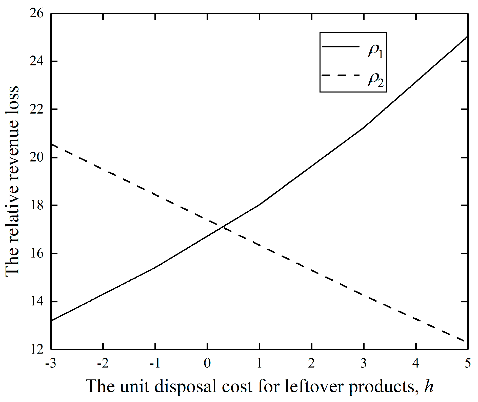
Define . and represent the relative losses of earning for the over-estimation and over-precision retailers, respectively. The greater the values of ρ1 and ρ2 are, the more unfavorable the overconfidence behavior is to the retailer.
We set the main parameters as follows:
,
, , and
, and let
follow the uniform distribution
U [−30,30]. We carried out the numerical studies in several parameter settings and obtained similar results, so we used such parameter values. The product is a perishable agricultural product (e.g., a fruit or vegetable), which is a daily necessity for human consumers. It has a large market and a low price, and the product cost
c is much smaller than the market scale
m. In general, for a perishable agricultural product, the parameters
s,
c, and
h have the same order of magnitude. We set the upper bound
U at a moderate value compared with
m. On the one hand, if the upper bound
U is very large, customer demand will be negative under extreme conditions. On the other hand, if the upper bound
U is very small, the impact of overconfidence will be negligible. Following [
30], we set the market sensitivity coefficient
k as 1.
We first study the effect of the overconfidence behavior on the optimal returns of the retailer under different parameter values given the level of overconfidence. In [
20], they found that the degrees of participants’ overconfidence observed in the newsvendor experiment were mainly in the interval
. We set the parameters of overconfidence at
. Next, we fix the unit production cost of the product while changing one of the two items of the unit shortage penalty cost and the unit surplus cost to observe changes in the retailer’s decisions and earning.
We set ; ; and and obtain the following results.
We make the following observations from the results in
Table 2: (1) Both over-estimation and over-precision will damage the retailer’s earning. (2) Under the over-estimation scenario, the retailer will set a higher retail price than that under the rational scenario, and it will order more than under the rational scenario, which leads to a decrease in its own earning. (3) As
h increases, the over-estimation retailer’s relative loss of earning will also rise because it needs to spend more to handle the surplus. (4) Under the over-precision scenario, the retail price is no different from that under the rational scenario, but the retailer will order less than under the rational scenario, which leads to a reduction in its own earning. (5) As
h increases, the risk of overstocking increases (being unable to sell means paying the cost
h), so the advantage of the rational retailer over the over-precision retailer decreases, and the relative earning loss of the over-precision retailer is reduced. (6) As
h increases, the rational, over-estimation, and over-precision retailers will stock less, and their prices will increase. The reason is that the retailer increases the price to compensate for the potential risk of having surplus stock while reducing the stock to cut down the surplus stock.
For the convenience of observation, we draw the curve of the relative earning loss of the overconfident retailer with changing h in the following:
As shown in
Figure 1, the velocity of
decreasing with
h is uniform. The growth of
with increasing
h is generally uniform, with a slightly faster growth trend.
We set ; and and obtain the following results.
The management implications of the results in
Table 3 are as follows: (1) As
c increases, the relative earning loss of the over-estimation retailer increases because it will order more than the rational retailer and spend more on the production cost. (2) As
c increases, the relative loss of earning of the over-precision retailer decreases. The over-precision retailer will order less than the rational retailer. Although such a behavior can make the over-precision retailer lose revenue because it cannot meet customers’ demand, its relative loss of earning will decrease when the production cost increases. (3) As
c increases, the rational, over-estimation, and over-precision retailers will choose to raise their retail prices and reduce their stocks available to cope with the increased costs.
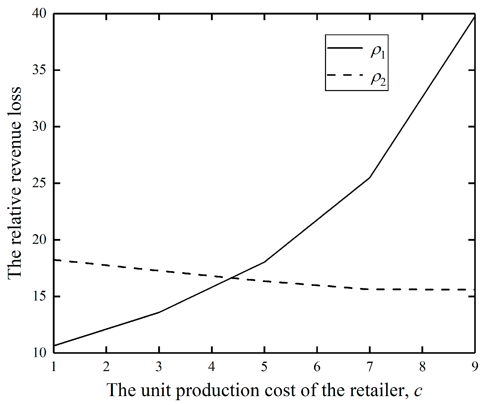
For the convenience of observation, we further draw the curve of the relative earning loss of the overconfident retailer with changing c in the following:
As shown in
Figure 2,
decreases with
c at an even slower rate.
increases with
at an increasingly faster rate.
We set ; ; and and obtain the following results.
We observe from the results in
Table 4 the following: (1) As
s increases, the relative earning loss of the over-estimation retailer increases, but the growth rate is slow because the retailer will order more than the rational retailer, with a low probability of stockout. (2) As
s increases, the relative loss of earning of the over-precision retailer increases, and the growth rate is much higher than that of the over-estimation retailer. This is because the over-precision retailer will order less than the rational retailer and is prone to be out of stock. Therefore, the relative earning loss rises with increasing shortage loss. (3) As
s increases, the rational, over-estimation, and over-precision retailers will choose to raise their retail prices to compensate for the potential shortage losses while increasing their orders to reduce the probability of shortage.
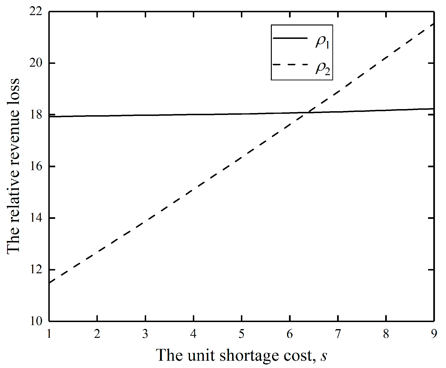
For the convenience of observation, we further draw the curve of the relative earning loss of the overconfident retailer with changing s in the following:
As shown in
Figure 3,
decreases with
c at an even, slow decline rate.
increases with
c at an increasingly faster rate.
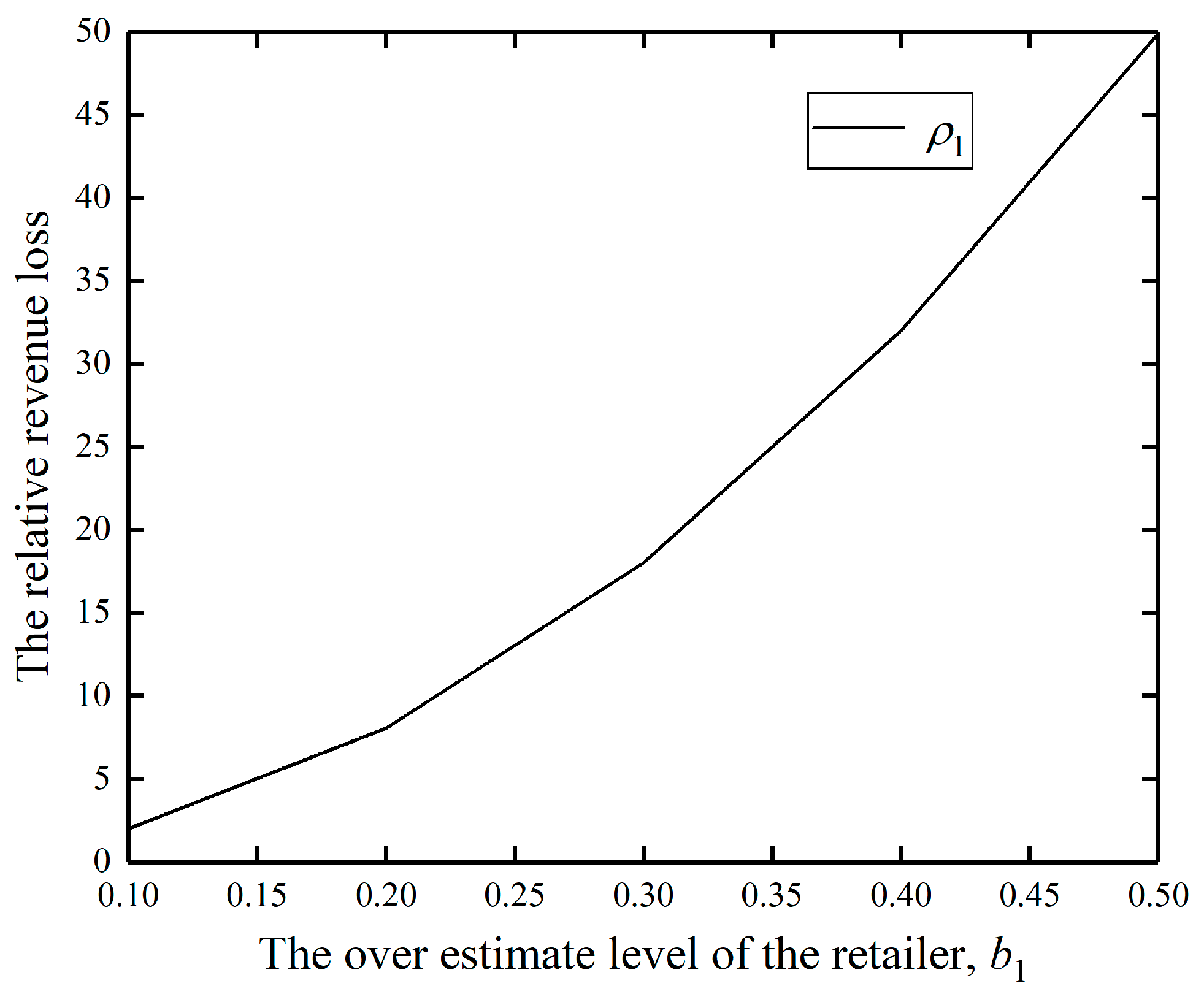
To further study the impact of the overconfidence level on the retailer’s earning loss, we set ; and and change and to observe changes in the retailer’s decisions and return.
We set
and
and obtain the following results in
Table 5.
We further draw the curve of over-estimation retailer’s relative earning loss with changing level of overconfidence in the following:
As shown in
Figure 4, with the increase of
, the over-estimation retailer and the rational retailer deviate further in their ordering, and the over-estimation retailer’s retail price increases further, which makes it hard to sell more products. Thus, the over-estimation retailer has a relatively higher earning loss.
We set
and
and obtain the following results in
Table 6.
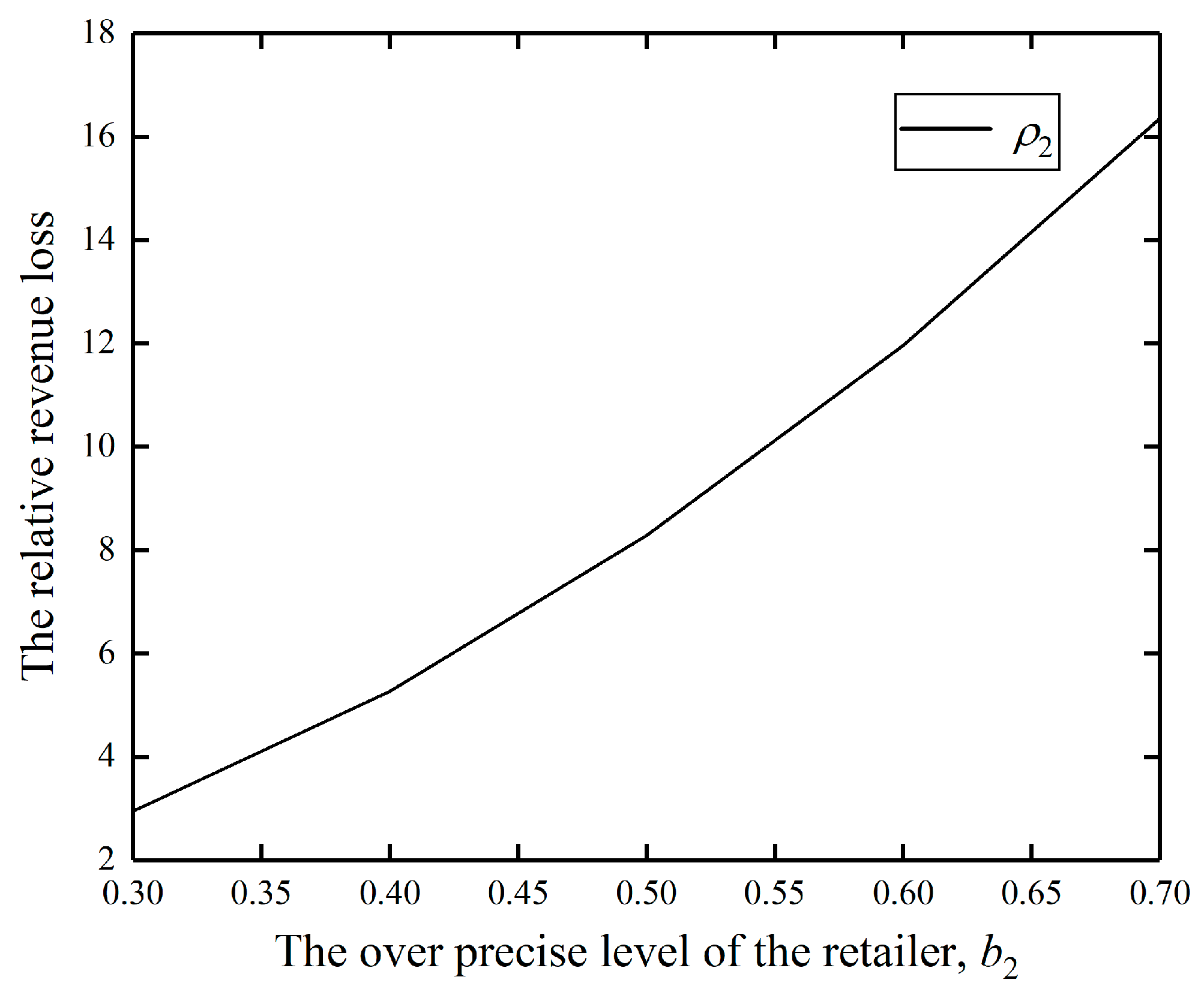
We further draw the curve of over-precision retailer’s relative earning loss with changing level of overconfidence in the following.
As shown in
Figure 5, with the increase of
, the ordering of the over-precision retailer will be further reduced, which leads to failure in meeting customers’ demand. The retailer needs to pay more for understocking. As a result, the relative loss of earning of the over-precision retailer increases.


