Article

Back Analysis of Surrounding Rock Parameters in Pingdingshan Mine Based on BP Neural Network Integrated Mind Evolutionary Algorithm

1
State Key Laboratory of Coking Coal Exploitation and Comprehensive Utilization, China Pingmei Shenma Group, Pingdingshan 467000, China
2
School of Civil Engineering, Wuhan University, Wuhan 430072, China
3
State Key Laboratory of Geomechanics and Geotechnical Engineering, Institute of Rock and Soil Mechanics, Chinese Academy of Sciences, Wuhan 430072, China
*
Author to whom correspondence should be addressed.
Mathematics 2022, 10(10), 1746; https://doi.org/10.3390/math10101746
Submission received: 21 March 2022 / Revised: 17 May 2022 / Accepted: 18 May 2022 / Published: 20 May 2022

Abstract

:
The mechanical parameters of surrounding rock are an essential basis for roadway excavation and support design. Aiming at the difficulty in obtaining the mechanical parameters of surrounding rock and large experimental errors, the optimized BP neural network model is proposed in this paper. The mind evolutionary algorithm can adequately search the optimal initial weights and thresholds, while the neural network has the advantage of strong nonlinear prediction ability. So, the optimized BP neural network model (MEA-BP model) takes advantage of the two models. It can not only avoid the local extreme value problem but also improve the accuracy and reliability of the prediction results. Based on the orthogonal test method and finite element analysis method, training samples and test samples are established. The nonlinear relationship between rock mechanical parameters and roadway deformation is established by the BP model and MEA-BP model, respectively. The importance analysis of the three input variables shows that the ∆D is the most important input variable, while ∆BC has the smallest impact. The comparison of prediction performance between the MEA-BP model and BP model demonstrates that the optimized initial weights and thresholds can improve the accuracy of prediction value. Finally, the MEA-BP model has been well applied to predicting the mechanical parameter for the surrounding rock in the Pingdingshan mine area, which proves the accuracy and reliability of the optimized model.

1. Introduction

The mechanical parameters of surrounding rock are the most important indexes in underground engineering construction. The rock mass is a typical anisotropy and heterogeneity medium with fissures, fractures, joints, bedding planes, and faults [1]. Therefore, the evaluation and prediction of rock mechanical parameters is still a challenge [2]. Researchers and technicians have developed various methods for the determination of rock mechanical parameters [3]. It includes direct measurement, indirect evaluation, laboratory test, numerical analysis, etc. [2,4,5,6,7,8]. Due to the limitations of sample size, quantity and cost, it cannot accurately reflect the variation of rock mass mechanical parameters via laboratory tests. What is more, the surrounding rock and support structure will change slowly with stress and time. It is difficult to dynamically evaluate the mechanical properties of surrounding rock and supporting structures by the traditional method. With the application of computer technology, depth learning has become a new method to solve geotechnical problems [9,10,11]. It can make full use of the data easily obtained but also the dynamic prediction and evaluation. Neural networks, support vector machines, decision trees, Bayesian classifiers, and other algorithms have been used in various rock mass engineering [9,12,13,14].
BP neural network has the advantage of strong nonlinear prediction ability, which has been widely used [15,16]. For example, Suman et al. [17] evaluate the safety of slope with functional networks, multivariate adaptive regression splines, and multigene genetic programming. Based on the literature data, the multivariate adaptive regression splines model has the best prediction performance in comparison with other models. To evaluate the stability of a rock slope with interlayered rocks, Wu et al. [18] predict the peak shear strength by a neural network approach. It also considers the effect of joint wall strength combination, normal stress, and joint roughness. The results show a good prediction precision when compared with the experimental data. Salsani et al. [19] reveal that the most critical factor on the road headed performance is the unconfined compressive strength. The nonlinear relation between the unconfined compressive strength, Brazilian tensile strength, rock quality designation, alpha angle, and the road headed performance could be accurately predicted by an artificial neural network. Based on the data of dynamic wave velocity, point load index, slake durability index, and density, the rock strength can also be predicted by an artificial neural network [20]. The hybrid model is proposed by Dai et al. [21], which combines the improved artificial fish swarm algorithm of strong global searching ability and the back propagation algorithm of strong local search ability. The preciseness of hybrid model is better than the other models. An optimized probabilistic neural network (PNN) model is proposed by Feng et al. [22], which makes full use of the mean impact value algorithm (MIVA) and the modified firefly algorithm (MFA). Then, the proposed model shows a good prediction ability in the evaluation of rock burst for the deep tunnels.
The above studies have confirmed the application of neural networks. However, the different initial weights and thresholds of the BP neural network will lead to non-convergence or local extreme value and even a large prediction error. The main reason is that the initial weights and thresholds of BP neural network are randomly generated, which affects the performance of the model. Therefore, selecting appropriate initial weights and thresholds is very important for the accuracy of the prediction model. Mind evolutionary algorithm (MEA) draws on the idea of population and evolution in genetic algorithms. It introduces the process of convergence and alienation, which has a strong ability for global optimization. In other words, the MEA model can search for the optimal initial weights and thresholds. Therefore, some scholars use the MEA model to optimize the performance of the BP neural network. Then an MEA-BP neural network is established and applied in the prediction model, which achieves a good result [23,24,25]. However, the application of the MEA-BP method in the prediction of surrounding rock parameters is still less.
Based on studying the prediction method of surrounding rock mechanical parameters, the mind evolutionary algorithm and BP neural network are introduced and combined firstly. Based on the Matlab program, the optimized BP model (MEA-BP model) is proposed in this paper. Then, the important analysis and comparison for the MEA-BP method are carried out, demonstrating the validity of proposed method. Finally, based on the observed displacement of roadway in the Pingdingshan mining area, the mechanical parameters of surrounding rock are predicted and evaluated, which is expected to provide a reference and basis for the long-term stability analysis of deep surrounding rock.

2. Methodology

2.1. Prediction Method

According to the Mohr-Coulomb criterion, the mechanical parameters of surrounding rock are major factors affecting the stability of roadway surrounding rock. It includes elastic modulus (E), cohesion (c), and friction Angle (φ). On the other hand, surrounding rock deformation is highly sensitive to these three parameters, which is difficult to obtain accurately [26]. Therefore, the deformation of surrounding rock U (u1, u2, u3, …) can be defined as a function of mechanical parameters (E, c, φ). The nonlinear relationship between surrounding rock deformation and mechanical parameters can be expressed as:
U ( u 1 , u 2 , u 3 , ) = f ( E , c , φ )
In engineering applications, the deformation of surrounding rock can be measured easily, while it is contrary to the mechanical parameters of rock mass. Therefore, it is an innovative method to evaluate the mechanical parameters based on surrounding rock deformation. So, the relationship between surrounding rock deformation and mechanical parameters is very significant for the accuracy of prediction results. Due to the nonlinear relationship between surrounding rock mechanical parameters and deformation, it is very difficult to solve in theory.
The neural network has the advantages of strong learning ability and good plasticity, which has been widely used in nonlinear fitting and prediction. However, most neural networks are based on gradient descent algorithms. The convergence speed is slow, and the training time is too long. What is more, the selection of initial weights and thresholds seriously affects the convergence and accuracy of the neural networks, which is prone to local extreme value. Therefore, the mind evolutionary algorithm is adopted in this paper, which is aimed at the optimized initial parameters of the BP neural network. Then, the relationship between surrounding rock deformation and mechanical parameters is established by the optimized BP model. This method can avoid the local extreme value problem but also improve the accuracy and reliability of the prediction model.

2.2. The Optimized BP Model

2.2.1. BP Neural Network Model

The BP neural network model is the most intuitive and widely used among many artificial neural network models. The BP neural network model is a feed-forward multilayer perceptron neural network and error backpropagation learning algorithms. A representative BP neural network model consists of three layers: an input layer, a hidden layer, and an output layer [27], as shown in Figure 1. The learning process can be divided into two parts: model forward propagation and error back propagation. In the forward propagation, the input sample enters the input layer and then propagates to the output layer after being processed by the hidden layer. The computation process [15] between input and output can be expressed as:
Y ¯ = f o u t p u t j = 1 H w k j ( f h i d d e n ( i = 1 I w j i X i + b j ) + b k )
Then, the error is calculated by:
E = 1 N n = 1 N ( Y ¯ n Y n ) 2 n = 1 , 2 , 3 , , N
where, i and H represent the numbers of the input sample and hidden sample; bj and bk represent the basis of hidden and output layer; foutput and fhidden represent the transfer functions for the hidden and output neurons; wji represents the weights connecting the input layer and hidden layer; wkj represents the weights between the hidden layer and output layer; Y ¯ n and Yn represent the predicted and actual output for the training sample.
If the error exceeds the tolerance, then the output error will be propagated back to the input layer via the hidden layer. Repeated training and learning are carried out until it meets the requirement [28].

2.2.2. Mind Evolutionary Algorithm

The mind evolutionary algorithm (MEA) inherits the concepts of “group” and “evolution” from the genetic algorithm (GA). It also has important innovations. Inspired by man’s mind action attributes under certain social environments, MEA comes up with “similar-taxis” and “dissimulation” [29]. The population of MEA consists of several groups surviving around the environment. Those groups are divided into superior groups and temporary groups randomly. Each group includes some individuals according to their uniform distribution (Figure 2).
The strategy of MEA is searching for the individual which has the highest score as a superior individual. Then, other individuals with the highest score as temporary individuals. The MEA designs two stages to realize the optimization goal [24]. Through the “similar-taxis”, the local information and local optimization are obtained. While the “dissimilation” operation conducts a global search and makes ‘‘exploration’’ in the whole search space. Through the “similar-taxis” and “dissimilation” alternately, MEA can achieve the balance of exploration and exploitation. The evolutionary process is described as the follows:
(a)
The population of MEA consists of several groups surviving around the environment. Those groups are divided into superior groups and temporary groups randomly. Each group includes several individuals according to their uniform distribution.
(b)
MEA searches for the individual with the highest score as a superior individual. At the same time, other individuals which have the highest score as temporary individuals. Each superior individual and temporary individual as the center to generate the superior subgroups and temporary subgroups.
(c)
The “similar-taxis” process is completed within the subgroups. The population maturity discriminant function is used to confirm whether the subgroup is mature. If it is, the mature subgroup stops this process. Then, the score of the optimal individual is regarded as the group score. The immature subgroup will produce subgroups with new centers. The above process will be repeated until they mature.
(d)
The disassimilation process is completed globally. If the score of the temporary subgroup is higher than that of the optimal subgroup, this process is carried out. Then, individuals in the temporary subgroup with a high score will replace those with a low score. At the same time, the individuals in the optimal subgroup are released. A new temporary subgroup is reconstructed in the global space.
(e)
Repeating the above process until the score of the optimal group is so high that it is impossible to increase. Then, the algorithm is convergent, and the winner of the superior group is just the global optimization.
Obviously, MEA takes advantage of the similar-taxis and the dissimilation to make the local search and global search alternately. Moreover, MEA designs billboards to record the evolutionary information that will guide the evolution in turn. So, MEA can make use of its directional search advantage, which is good for the search of optimal initial weights and thresholds. Currently, MEA has successfully applied to many optimization problems [25].

2.3. Combined Prediction Method

The MEA can search for the best initial weights and thresholds quickly and accurately. While the neural network has the advantages of high calculation precision and controllable error. So, the combination of two models is proposed to predict rock parameters. In other words, the optimal initial weights and thresholds value is obtained by the mind evolutionary algorithm. Then, the optimized initial value is used in the BP neural network model, which can improve the convergence speed and fitting accuracy of the BP neural network. Finally, an MEA-BP model is established based on the Matlab program.
In addition to the prediction model, the data of training and verification for the prediction model is another key point, which determined the accuracy of the predict value. The common method for the establishment of training data and verification data is field monitoring or numerical analysis [13,14,30,31]. Due to the complex engineering conditions, the filed data cannot acquired easily. Numerical analysis is an efficient method for the analysis of influence law of rock mechanical, which has been widely used in the back analysis of surrounding rock [31]. At the same time, the orthogonal experimental design method is also adopted in the establishment of training data. Orthogonal experimental design method is a representative method for the study of multi factors and levels. It can reflect the influence of all factors and levels, which is appropriate for the study of rock engineering. Thus, both orthogonal experimental design method and finite element method (FLAC3D) are adopted in the establishment of training sample and test sample.
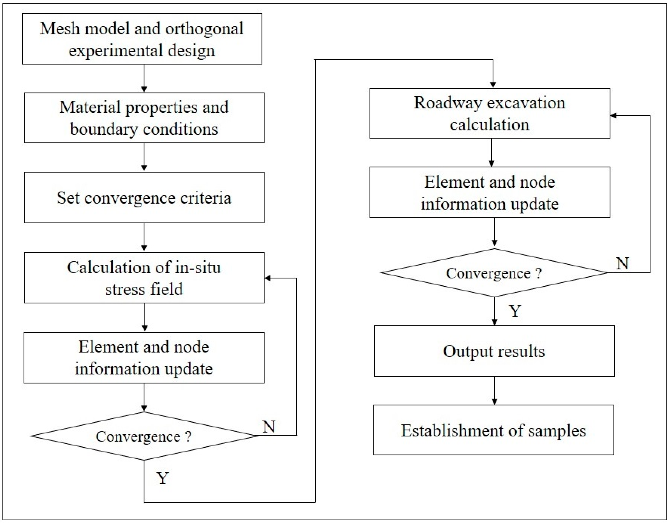
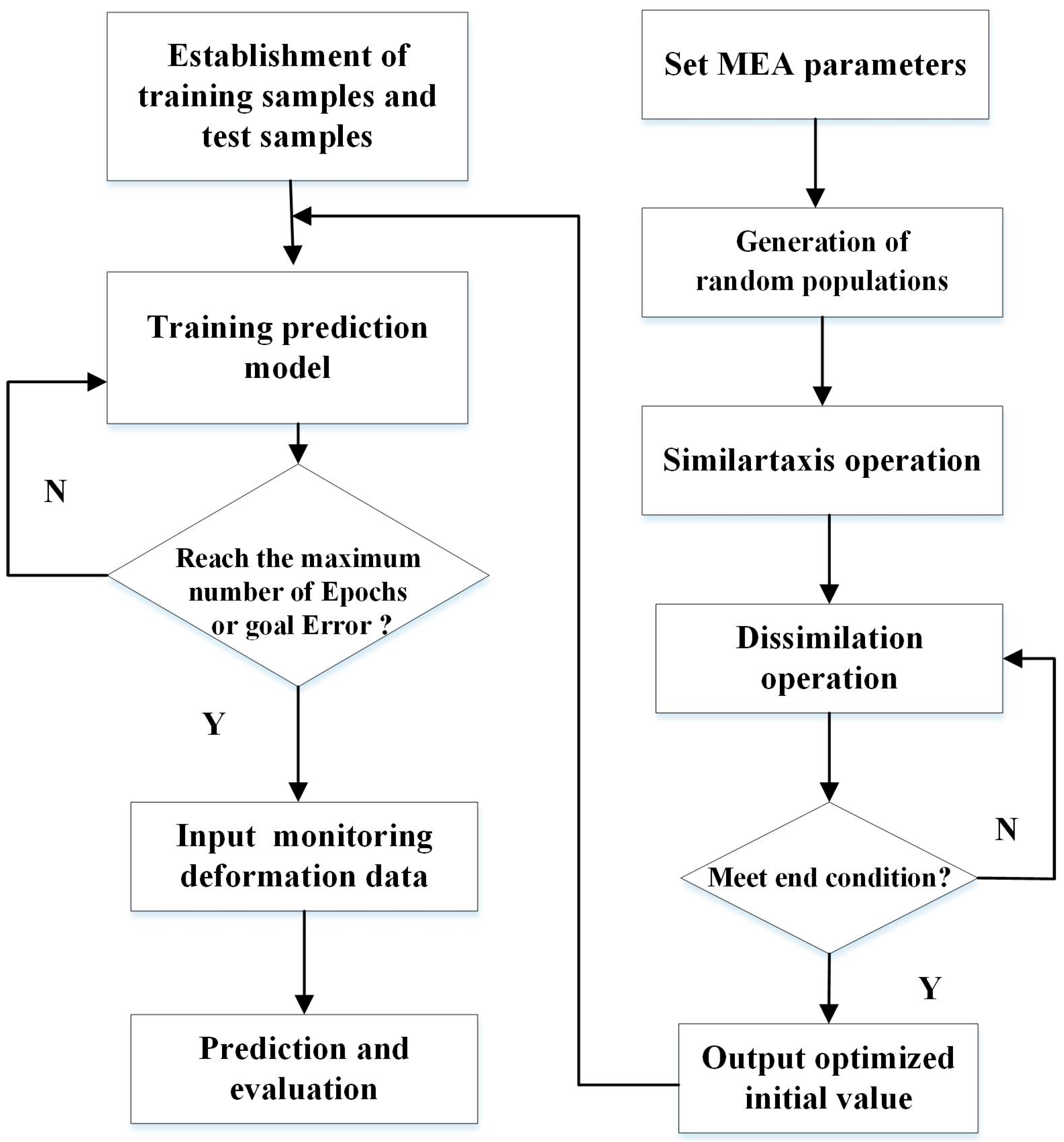
Based on the training data and predicted model, the nonlinear relationship between mechanical parameters and deformation of surrounding rock can be established. The steps to develop a combined prediction model (MEA-BP model) are illustrated in Figure 3 and Figure 4.
Step 1: The establishment of a training sample. The orthogonal experimental design method is used to determine the test scheme based on three rock mechanical parameters. Then, the deformation results of surrounding rock under different mechanical parameters are simulated by the finite element method (FLAC3D). The deformation results and mechanical parameters of surrounding rock are regarded as the input and output variable values for the training sample, respectively (Figure 3).
Step 2: Determination of BP network. The parameters of the input layer, output layer, and hidden layer were determined.
Step 3: Setting MEA parameters. The number of iterations, initial population, superior subpopulation, temporary subpopulation, network weights, and threshold are determined.
Step 4: Generation of random populations. The optimized weights and thresholds are coded according to the MEA parameters. Then, the superior subgroups and temporary subgroups are generated.
Step 5: The similar taxis operation is performed in each subgroup until the subgroup is mature. The score of the optimal individual is used as the score of the subgroup.
Step 6: The dissimilation operation is performed between the superior and temporary subgroups.
Step 7: Output the superior individual when the iterations operations or the optimal global individual is found. If the above conditions are not satisfied, return to step 3.
Step 8: The optimized initial weights and thresholds are assigned to the BP network. The MEA-BP model trains the nonlinear relationship between the deformation and rock mechanical parameters.
Step 9: Prediction and evaluation. The observed displacement value is used to predict rock mechanical parameters by the MEA-BP model. Then, the predicted displacement is obtained by finite element numerical analysis methods. Finally, the comparison and evaluation between the predicted displacement and the observed value are carried out (Figure 4).

3. Application of Prediction Model

3.1. Geological and Numerical Model

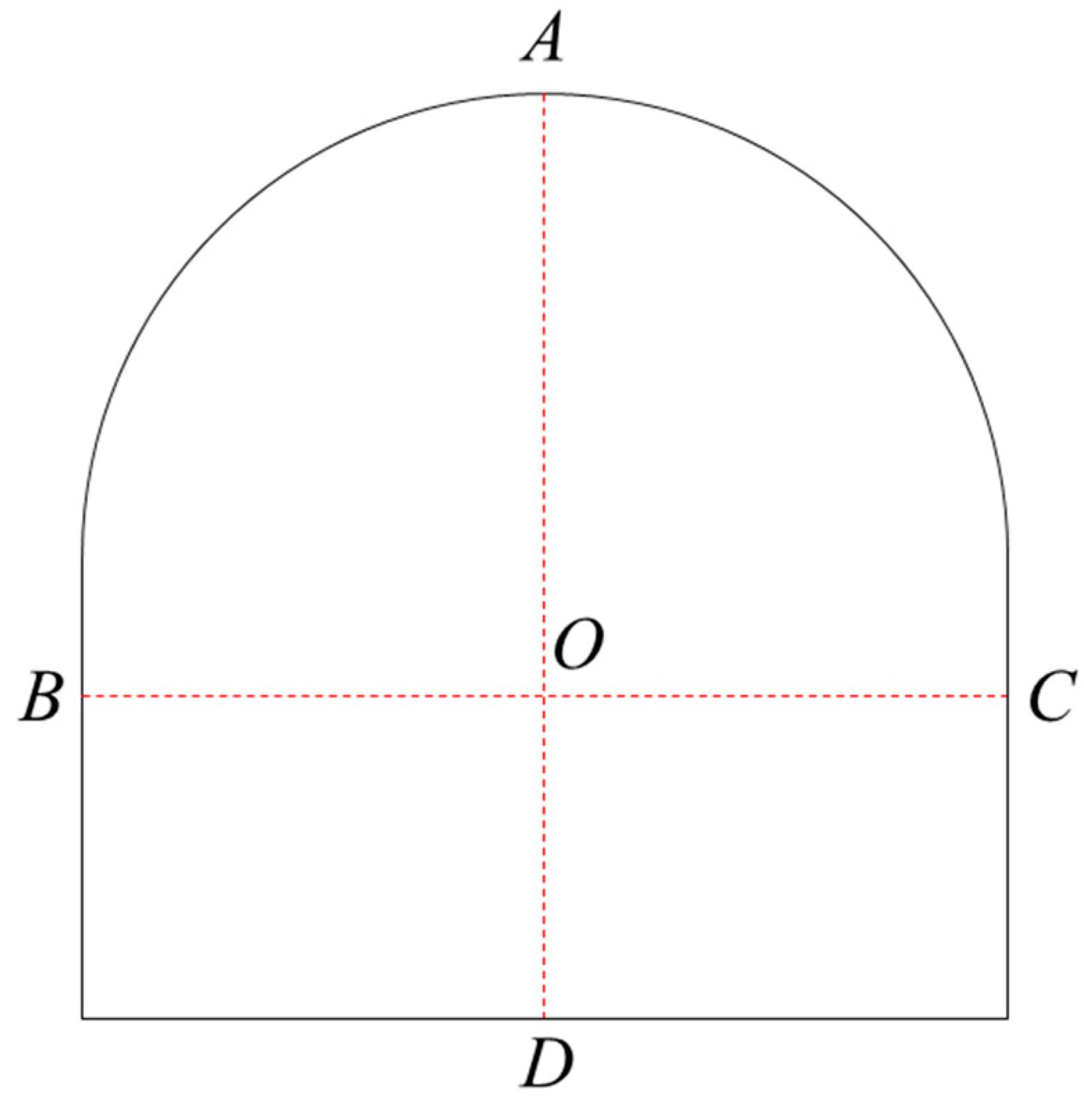
The study roadway is located in the No.10 mine of the Pingdingshan mining area. The rock stratum of the roadway is a sandy mudstone layer. The overall geological structure is stable, and no obvious fissure water is found. The roadway section is a straight-wall arch, with a width of 5.6 m, a height of 4.5 m, and a radius of 1.7 m. According to the classification of surrounding rock, the surrounding rock where the roadway is located belongs to class Ⅲ~Ⅴ. The basic quality (BQ) rating system is most widely used as an empirical method for rock mechanical parameters [32]. Then, the range of elastic modulus (E), cohesion (c), and friction Angle (φ) is calculated by the BQ rating system. Other parameters are determined by the laboratory test results, as shown in Table 1. The measurement of in-situ stress shows that the σx = 30.81 MPa, σy = 28.78 MPa, σz = 27.04 MPa. To quantitatively analyze the deformation of surrounding rock, the displacement of point A and point D (∆A and ∆D) is regarded as the vertical deformation value. At the same time, the relative displacement of point B and point C (∆BC) is selected as the horizontal deformation value, as shown in Figure 5. The displacement of roadway surrounding rock is measured by a laser range finder (Figure 6).
The finite element analysis method (FLAC3D) is used to simulate the roadway deformation with different rock mechanical parameters to establish the training samples. The rock mechanical parameters are determined by Table 1. The Elasticity modulus, cohesion and friction angle are regarded as the variable for the establishment of training data and verification data. The other parameters are constant, which can refer to the Table 1. In addition, the Mohr-Column criterion is adopted. The model range must be sufficiently large to minimize the influence of boundary effects. Therefore, a 3D roadway numerical model with a size of 67.2 m × 60 m × 36 m is established, as shown in Figure 7. The element number of the numerical analysis model is 12,380. The upper part of the model is a free boundary, and the other boundaries are fixed. The three principal stresses are applied in the corresponding directions, and gravity is also considered. When the convergence value (ratio = 1 × 10⁻⁵) is reached, the equilibrium state can be considered to be reached.

3.2. Establishment of Training Sample

Orthogonal experimental design is an experimental method for studying multi-factor and levels. According to the principle of orthogonal design, some representative points are selected for the test, which has the characteristics of “uniform dispersion, neat and comparable”. The orthogonal test method has high efficiency, which can quickly determine the influence degree of relevant factors on deformation. So, the orthogonal experimental design method is used to construct the training samples for the prediction model. The rock mechanical parameter includes elastic modulus (E), cohesion (c), and friction angle (φ), which has eight levels, as shown in Table 2. After roadway excavation and timely support, the surrounding rock and support structure can be regarded as the overall structure. Therefore, the rock mechanical parameters described in this paper are the overall mechanical parameters of surrounding rock and support structure, which is also the basis for the analysis of surrounding rock after support.
Based on Table 2 and the orthogonal test design method (L64), 64 training samples are obtained by numerical analysis. Correspondingly, the deformation of roadway (∆A, ∆D, and ∆BC) with different rock mechanical properties is regarded as the input value for the training sample (Figure 3). The mechanical parameters of orthogonal experiments are regarded as the observed value. Then, the nonlinear relationship between the deformation and rock mechanical parameters of surrounding rock is obtained by the training sample. The nonlinear relationship obtained by the MEA-BP model can be used to predict of rock mechanical parameters. Finally, the evaluation of the prediction model can be carried out (Figure 4).

3.3. Importance Analysis of Input Variables

In addition to being interested in the prediction performance of the MEA-BP model, the importance of different input variables on the prediction performance is concerned, which increases the interpretability of the model. Permutation importance (PI) is a common indicator to measure the importance of input variables [33]. It has the advantages of being easy to understand and fast to calculate. The detailed procedure of importance analysis is introduced as follows:
(1)
Based on the BQ rating system, eight group mechanical parameters of test samples are generated by the random method. Then, the deformation of surrounding rock is obtained by the finite element numerical method. The data of test sample is shown in Table 3. The surrounding rock deformation results and mechanical parameters are regarded as the input value and observed value for the test samples.
(2)
Train the MEA-BP model based on the original training samples (L64). Then, the prediction of the test sample (Table 3) is obtained, and the RMSE is calculated by Equation (4).
R M S E = 1 N t = 1 N ( o b s e r v e d t p r e d i c t e d t ) 2
where, observedt represents the observed value; predictedt represents the predicted value; t represents the predicted variable, N represents the number of input variables.
(3)
Shuffle the ith input variable of the training samples in reverse order, and the others remain unchanged.
(4)
Train the MEA-BP model on the shuffled training samples. The prediction of the test sample and RMSE is calculated by Equation (4).
(5)
Calculate PI of the ith input variable using Equation (5);
P I i = R M S E i R M S E *
where, RMSEi and RMSE* are separately calculated on the shuffled training samples and original training samples; i (i = 1, 2, 3) represents the input variable (∆A, ∆D, ∆BC).
(6)
Repeat (3)~(4) until PI of all input variables (∆A, ∆D, ∆BC) is obtained. To be more intuitive, PI is standardized by Equation (6).
P I i * = P I i / i = 1 n P I i × 100 %
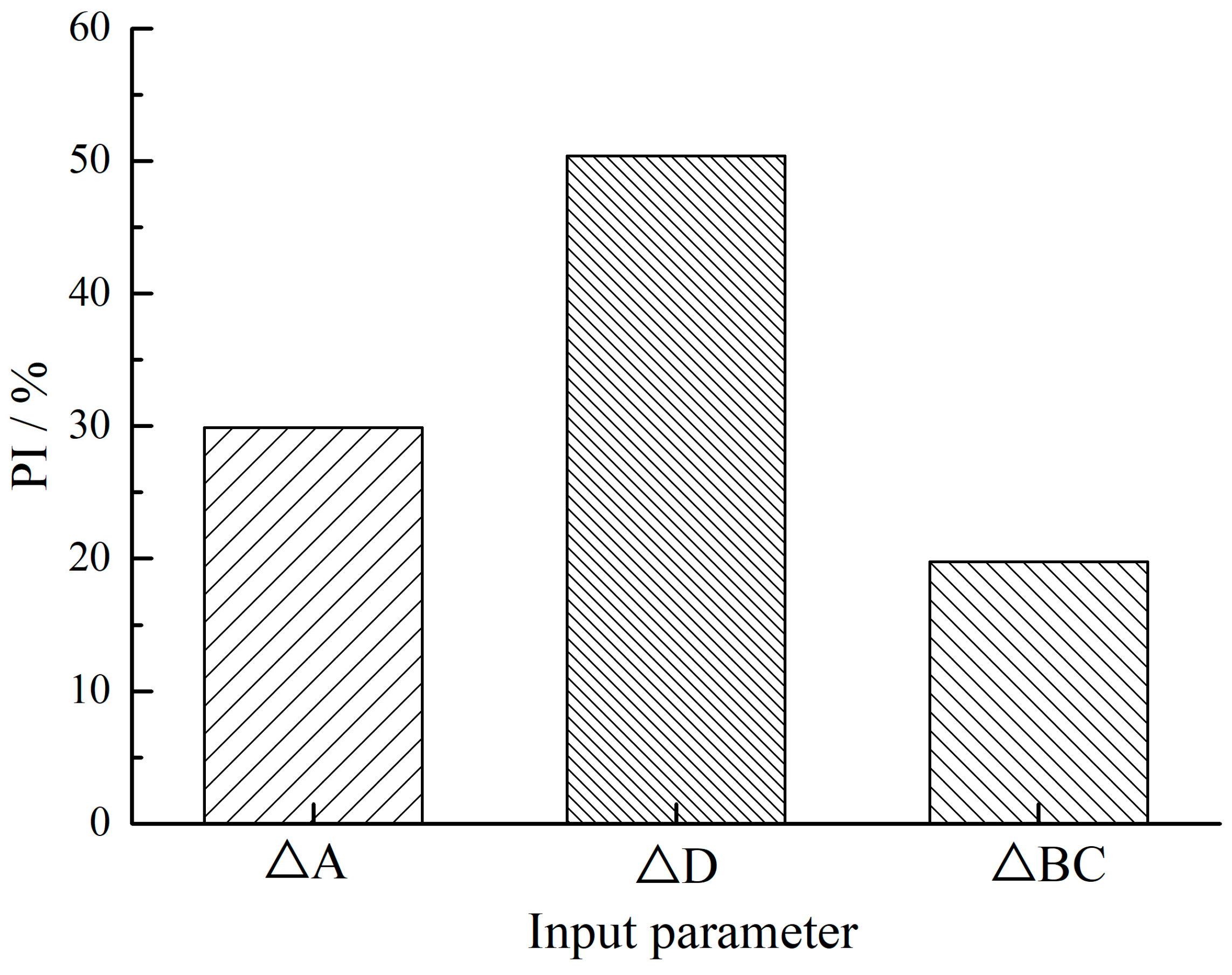
Firstly, the RMSE of three input variables (∆A, ∆D, ∆BC) for eight test samples is obtained (Table 4). The larger RMSE means a greater adverse effect. The range of RMSE* is 0.24~1.20, with an average of 0.58. Except the group 5, the RMSEi for other groups is larger than RMSE*. It indicates that the changes of the input value of training samples have a significant impact on the prediction results. The average of RMSE2 is the largest, while the RMSE1 is the second. The larger PI is, the more important the corresponding input variable. It can be seen that the PI* for ∆D, ∆A, and ∆BC is 49.93%, 30.30%, and 19.77%, respectively (Figure 8). In other words, the variation of PI* is consistent with the average of RMSE. Especially, the RMSE2 is the biggest of six test groups. What is more, the maximum value of RMSE is 10.62, which also belongs to RMSE2. So, it can be considered that the ∆D is the most important input variable, while the influence of ∆BC is the least.

3.4. Model Analysis

To verify the effectiveness of the proposed model, the mechanical parameters are predicted by the MEA-BP model and BP model, respectively. The data of test samples are shown in Table 4. The parameters of the two models are shown in Table 5. The η is the learning rate; S is population size; m is the maximal iterative number; Nt is the number of the temporary subgroup; Ns is the number of superior subgroups; g is the convergence error.
The nonlinear relationship between surrounding rock deformation and mechanical parameters is established during the modeling process by 64 sets of the training samples (L64). Based on the test sample (Table 3), the RMSE of three predicted mechanical parameters is calculated by Equation (4). The smaller RMSE means the more reliable accuracy. All RMSE of the predicted mechanical parameters of the MEA-BP model are smaller than that of the BP model (Figure 9). It indicates that selecting initial weights and thresholds can improve the convergence and accuracy of neural networks but also avoid local extreme value problems. Compared with the BP model, the declining ratio of RMSE for the MEA-BP model was about 48.89~79.91%. In other words, the predicted performance of the MEA-BP model is better than that of the BP model.
The relative error value (REV) is used for the detailed comparison of MEA-BP model and BP model. The definition of relative error value is:
R E V x = x * x 0 x 0 × 100 %
where, REVx represents the relative error value of the parameter x; x represents the parameter variable (E, c, φ); x0 represents the initial value of a parameter; x* represents the predicted value of a parameter.
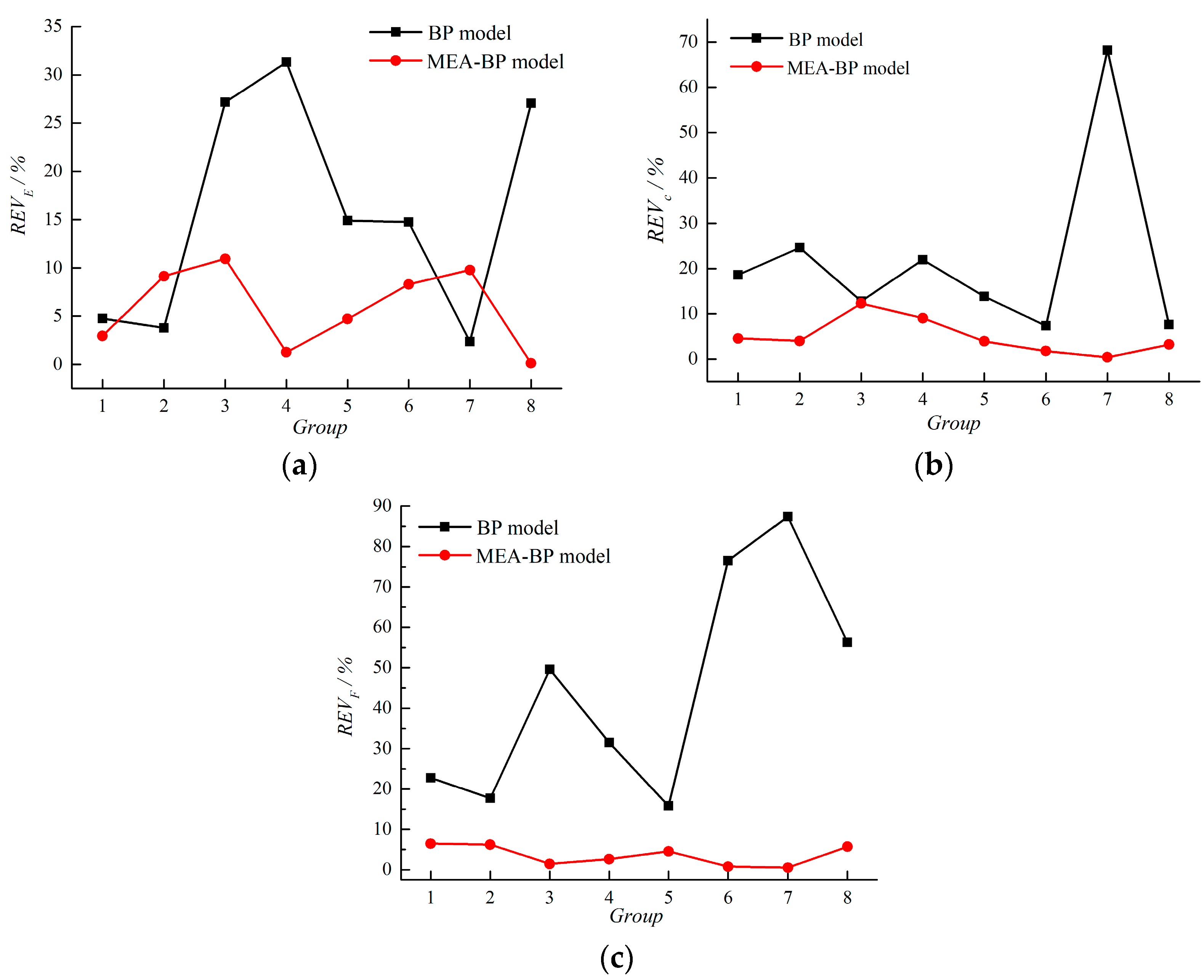
The REV of three parameters for the MEA-BP model and BP model is summarized in Figure 10. Compared with the BP model, the REV of three mechanical parameters is smaller when the MEA-BP model is adopted. Specifically, the REV of elastic modulus (E) is between 0.12~10.96% when the MEA-BP model is adopted. In contrast, it is 2.37~31.32% for the BP model. The cohesion and friction angle also shows the same change trend. The REV of cohesion and friction angle is less than 12.26% for the MEA-BP model, which is smaller than those of BP model. What is more, the REV of cohesion and friction angle is smaller than that of elastic modulus (Figure 10b,c).
Although, the nonlinear relationship between mechanical property and deformation of surrounding rock is inherent. However, the importance of different variables is different. So, the REV of some point is large. What is more, the different initial input value will lead to non-convergence or local extreme value and even a large prediction error when the BP neural network is adopted. Thus, the change of REV is irregular when the BP model is adopted. It is not only the key point of the prediction model but also the advantage of MEA-BP model. The sensitivity of input variables cannot be decreased, but the accuracy of the prediction can be improved when the MEA-BP model is adopted. In other words, the application of the mind evolutionary algorithm could improve prediction accuracy. The MEA-BP model has a better prediction performance than the BP model.

3.5. Application of MEA-BP Model

Based on Section 2, the MEA-BP model is used to predict mechanical parameters for the roadway in the Pingdingshan mine area. Firstly, two adjacent roadways are selected as monitoring roadways, and two sections are selected for each roadway. Then, the observed displacement value of roadway is shown in Table 6.
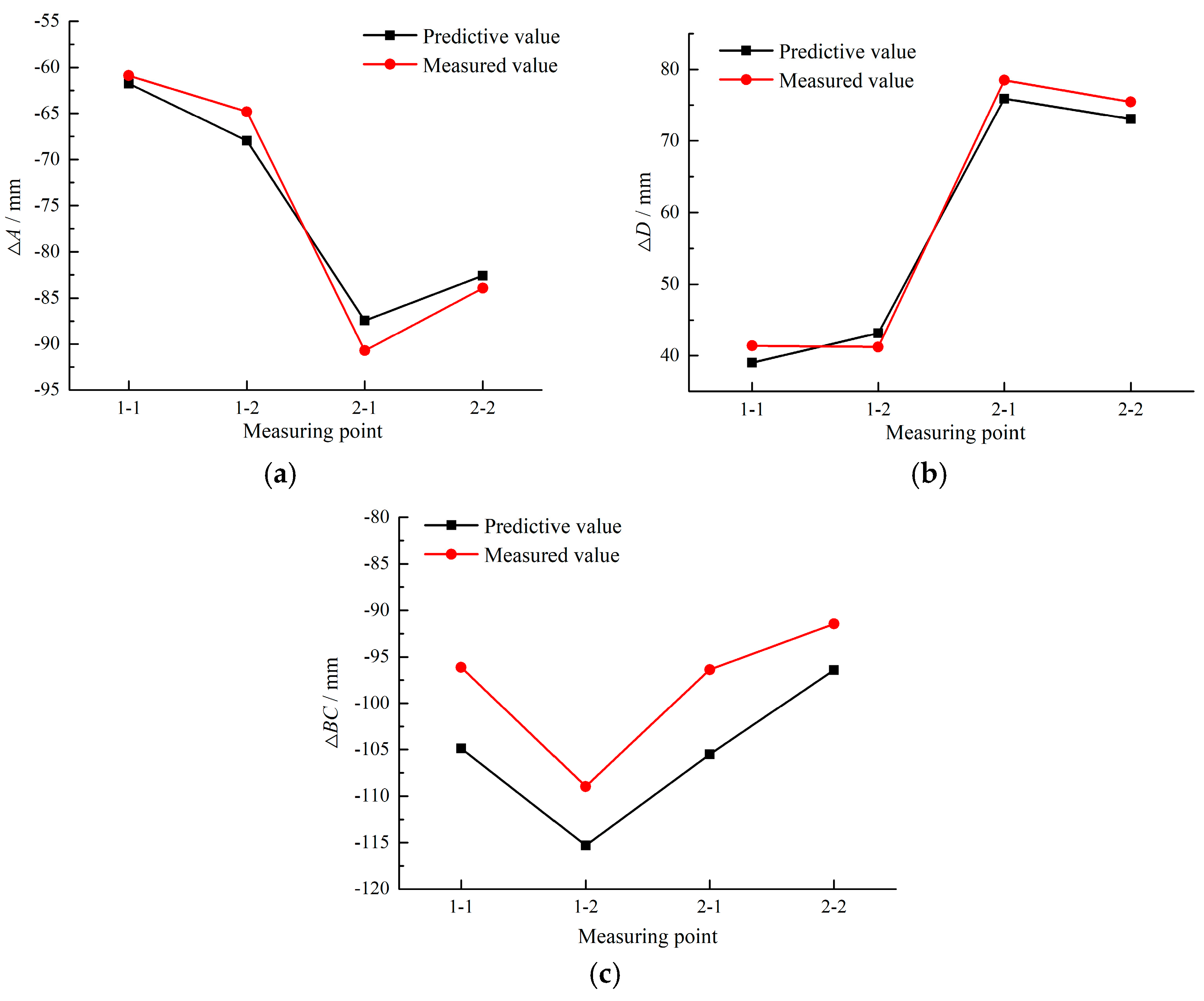
Based on the observed displacement value of roadway, the predicted rock mechanical parameter is obtained by the MEA-BP model. Then, the predicted deformation value of roadway is calculated via FLAC3D, which is used to compare the observed displacement (Figure 11). It can be seen that the REV of ∆A and ∆D ranges between 1.43% and 5.70%. The predicted value of ∆A and ∆D is basically consistent with the observed value. According to the important analysis of input variables (Section 3.3), the prediction result has the lowest sensitivity to ∆BC. So, it will result in a large error of ∆BC. What is more, the isotropic assumptions are adopted during the finite element analysis. It also does not consider the actual geological variation, such as fracture distribution. Therefore, the predicted deformation results of ∆BC are less than the observed values, but the REV of ∆BC is less than 9.1%. To sum up, the MEA-BP model can well predict the mechanical parameter.

4. Conclusions

To predict mechanical parameters for surrounding rock, an optimized BP prediction model is proposed in this paper. It makes use of the great search capability of the MEA model and the strong learning ability and plasticity of the BP model. Then, the orthogonal experimental design method and finite element method (FLAC3D) are adopted in the establishment of training sample and test sample. Thirdly, the nonlinear relationship between mechanical parameters and deformation of surrounding rock is obtained by BP model and MEA-BP model, respectively. Finally, the analysis show that the application of the mind evolutionary algorithm could improve prediction accuracy. It also has a better prediction performance in the application. The main conclusions are as follows:
(1)
To avoid the local extreme value and improve the convergence speed of the BP neural network model, the initial weights and thresholds are optimized by the mind evolutionary algorithm. So, the combination of the mind evolutionary algorithm and BP neural network is proposed in this paper, which is aimed at a good prediction of rock mechanical parameters.
(2)
Based on the orthogonal test method and finite element numerical method, training samples and test samples are established. The rock mechanical parameters are the observed value, while the deformation of surrounding rock (∆A, ∆D, ∆BC) is the input value. The nonlinear relationship between rock mechanical parameters and roadway deformation is established by the BP model and MEA-BP model, respectively.
(3)
The important analysis of different input variables for the MEA-BP model shows that the RMSE of ∆D is the largest. While the RMSE and PI for ∆BC are the smallest. It indicates that the ∆D is the most important input variable, while the influence of ∆BC is the least.
(4)
The comparison between the MEA-BP model and BP model shows that the RMSE value for the MEA-BP model is reduced by about 48.89~79.91%. What is more, the REV of the MEA-BP model is also smaller than that of the BP model. The MEA-BP model cannot decrease the sensitivity of input variables, but the accuracy of the prediction is improved. So, the prediction performance of the MEA-BP model is better than the BP model, which also demonstrates the advantages of the optimized initial weights and thresholds.
(5)
The MEA-BP model is used to predict mechanical parameters for roadways in the Pingdingshan mine area. The predicted deformation results are consistent with the observed value, which demonstrated the accuracy and reliability of the optimized model.

Author Contributions

Investigation, conceptualization and resources, J.Z.; writing, validation and formal analysis, P.L. and S.W.; software and methodology, X.Y.; project administration and funding acquisition Y.Z. and J.Z. All authors have read and agreed to the published version of the manuscript.

Funding

This work was supported by the Open Research Fund of State Key Laboratory of Coking Coal Exploitation and Comprehensive Utilization, China Pingmei Shenma Group (No. 4104022017110603) and National Natural Science Foundation of China (No. 51874275).

Institutional Review Board Statement

Not applicable.

Informed Consent Statement

Not applicable.

Data Availability Statement

Not applicable.

Acknowledgments

The wish to send acknowledgments to State Key Laboratory of Coking Coal Exploitation and Comprehensive Utilization (China Pingmei Shenma Group) for their help for the data collection and measurement. The authors also are very grateful to anonymous’ for their recommendations.

Conflicts of Interest

The authors declare no conflict of interest.

References

  1. Zhao, H.; Chen, B.; Li, S.; Li, Z.; Zhu, C. Updating the models and uncertainty of mechanical parameters for rock tunnels using Bayesian inference. Geosci. Front. 2021, 12, 101198. [Google Scholar] [CrossRef]
  2. Feng, X.-T.; Zhou, Y.-Y.; Jiang, Q. Rock mechanics contributions to recent hydroelectric developments in China. J. Rock Mech. Geotech. Eng. 2019, 11, 511–526. [Google Scholar] [CrossRef]
  3. Meng, F.; Wong, L.N.Y.; Zhou, H. Rock brittleness indices and their applications to different fields of rock engineering: A review. J. Rock Mech. Geotech. Eng. 2021, 13, 221–247. [Google Scholar] [CrossRef]
  4. Han, X.; Li, W.; Li, X.; Zhu, Z. Virtual reality assisted techniques in field tests and engineering application of the mechanical parameters of a horizontally layered rock mass. Alex. Eng. J. 2022, 61, 4027–4039. [Google Scholar] [CrossRef]
  5. Liu, H.; Liu, Q.; Ma, H.; Fish, J. A novel GPGPU-parallelized contact detection algorithm for combined finite-discrete element method. Int. J. Rock Mech. Min. Sci. 2021, 144, 104782. [Google Scholar] [CrossRef]
  6. Salmi, E.F.; Sellers, E.J. A review of the methods to incorporate the geological and geotechnical characteristics of rock masses in blastability assessments for selective blast design. Eng. Geol. 2021, 281, 105970. [Google Scholar] [CrossRef]
  7. Rostamsowlat, I.; Evans, B.; Kwon, H.J. A review of the frictional contact in rock cutting with a PDC bit. J. Pet. Sci. Eng. 2022, 208, 109665. [Google Scholar] [CrossRef]
  8. Schaefer, L.N.; Kereszturi, G.; Villeneuve, M.; Kennedy, B. Determining physical and mechanical volcanic rock properties via reflectance spectroscopy. J. Volcanol. Geotherm. Res. 2021, 420, 107393. [Google Scholar] [CrossRef]
  9. Lawal, A.I.; Kwon, S. Application of artificial intelligence to rock mechanics: An overview. J. Rock Mech. Geotech. Eng. 2021, 13, 248–266. [Google Scholar] [CrossRef]
  10. Liu, K.; Liu, B.; Fang, Y. An intelligent model based on statistical learning theory for engineering rock mass classification. Bull. Eng. Geol. Environ. 2018, 78, 4533–4548. [Google Scholar] [CrossRef]
  11. Barnoud, A.; Cayol, V.; Lelièvre, P.G.; Portal, A.; Labazuy, P.; Boivin, P.; Gailler, L. Robust Bayesian Joint Inversion of Gravimetric and Muographic Data for the Density Imaging of the Puy de Dôme Volcano (France). Front. Earth Sci. 2021, 8, 575872. [Google Scholar] [CrossRef]
  12. Hajihassani, M.; Jahed Armaghani, D.; Kalatehjari, R. Applications of Particle Swarm Optimization in Geotechnical Engineering: A Comprehensive Review. Geotech. Geol. Eng. 2017, 36, 705–722. [Google Scholar] [CrossRef]
  13. Yin, X.; Liu, Q.; Huang, X.; Pan, Y. Perception model of surrounding rock geological conditions based on TBM operational big data and combined unsupervised-supervised learning. Tunn. Undergr. Space Technol. 2022, 120, 104285. [Google Scholar] [CrossRef]
  14. Yin, X.; Liu, Q.; Huang, X.; Pan, Y. Real-time prediction of rockburst intensity using an integrated CNN-Adam-BO algorithm based on microseismic data and its engineering application. Tunn. Undergr. Space Technol. 2021, 117, 104133. [Google Scholar] [CrossRef]
  15. Liu, B.; Wang, R.; Zhao, G.; Guo, X.; Wang, Y.; Li, J.; Wang, S. Prediction of rock mass parameters in the TBM tunnel based on BP neural network integrated simulated annealing algorithm. Tunn. Undergr. Space Technol. 2020, 95, 103103. [Google Scholar] [CrossRef]
  16. Yin, X.; Liu, Q.; Pan, Y.; Huang, X. A novel tree-based algorithm for real-time prediction of rockburst risk using field microseismic monitoring. Environ. Earth Sci. 2021, 80, 504. [Google Scholar] [CrossRef]
  17. Suman, S.; Khan, S.Z.; Das, S.K.; Chand, S.K. Slope stability analysis using artificial intelligence techniques. Nat. Hazards 2016, 84, 727–748. [Google Scholar] [CrossRef]
  18. Wu, Q.; Xu, Y.; Tang, H.; Fang, K.; Jiang, Y.; Liu, C.; Wang, X. Peak shear strength prediction for discontinuities between two different rock types using a neural network approach. Bull. Eng. Geol. Environ. 2018, 78, 2315–2329. [Google Scholar] [CrossRef]
  19. Salsani, A.; Daneshian, J.; Shariati, S.; Yazdani-Chamzini, A.; Taheri, M. Predicting roadheader performance by using artificial neural network. Neural Comput. Appl. 2013, 24, 1823–1831. [Google Scholar] [CrossRef]
  20. Sarkar, K.; Tiwary, A.; Singh, T.N. Estimation of strength parameters of rock using artificial neural networks. Bull. Eng. Geol. Environ. 2010, 69, 599–606. [Google Scholar] [CrossRef]
  21. Dai, B.; Gu, H.; Zhu, Y.; Chen, S.; Rodriguez, E.F.; Geem, Z.W. On the Use of an Improved Artificial Fish Swarm Algorithm-Backpropagation Neural Network for Predicting Dam Deformation Behavior. Complexity 2020, 2020, 5463893. [Google Scholar] [CrossRef]
  22. Feng, G.; Xia, G.; Chen, B.; Xiao, Y.; Zhou, R. A Method for Rockburst Prediction in the Deep Tunnels of Hydropower Stations Based on the Monitored Microseismicity and an Optimized Probabilistic Neural Network Model. Sustainability 2019, 11, 3212. [Google Scholar] [CrossRef] [Green Version]
  23. Kordnaeij, A.; Kalantary, F.; Kordtabar, B.; Mola-Abasi, H. Prediction of recompression index using GMDH-type neural network based on geotechnical soil properties. Soils Found. 2015, 55, 1335–1345. [Google Scholar] [CrossRef] [Green Version]
  24. Wang, W.; Tang, R.; Li, C.; Liu, P.; Luo, L. A BP neural network model optimized by Mind Evolutionary Algorithm for predicting the ocean wave heights. Ocean. Eng. 2018, 162, 98–107. [Google Scholar] [CrossRef]
  25. Gobeyn, S.; Mouton, A.M.; Cord, A.F.; Kaim, A.; Volk, M.; Goethals, P.L.M. Evolutionary algorithms for species distribution modelling: A review in the context of machine learning. Ecol. Model. 2019, 392, 179–195. [Google Scholar] [CrossRef]
  26. Yu, J.; Zhang, Q.; Xu, W.; Wang, R.; Zhang, H. Study on Unloading Relaxation Characteristics of Columnar Jointed Rock Masses Based on Displacement Back Analysis. Front. Earth Sci. 2021, 9, 665275. [Google Scholar] [CrossRef]
  27. Ocak, I.; Seker, S.E. Calculation of surface settlements caused by EPBM tunneling using artificial neural network, SVM, and Gaussian processes. Environ. Earth Sci. 2013, 70, 1263–1276. [Google Scholar] [CrossRef]
  28. Zhang, C.; Li, J.-z.; He, Y. Application of optimized grey discrete Verhulst—BP neural network model in settlement prediction of foundation pit. Environ. Earth Sci. 2019, 78, 441. [Google Scholar] [CrossRef]
  29. Jie, J.; Zeng, J.; Han, C. An extended mind evolutionary computation model for optimizations. Appl. Math. Comput. 2007, 185, 1038–1049. [Google Scholar] [CrossRef]
  30. Yin, X.; Gao, F.; Wu, J.; Huang, X.; Pan, Y.; Liu, Q. Compressive strength prediction of sprayed concrete lining in tunnel engineering using hybrid machine learning techniques. Undergr. Space 2021, 6, 1–16. [Google Scholar] [CrossRef]
  31. Rohola, H.; Jamal, R.; Jürgen, S.; Yilmaz, O.; Babak, S. Prediction of TBM jamming risk in squeezing grounds using Bayesian and artificial neural networks. J. Rock Mech. Geotech. Eng. 2021, 12, 21–31. [Google Scholar]
  32. Cui, Z.; Sheng, Q.; Zhang, G.-m.; Liu, H. A modified rock mass classification considering seismic effects in the basic quality (BQ) system. Bull. Eng. Geol. Environ. 2021, 80, 2249–2260. [Google Scholar] [CrossRef]
  33. Yin, X.; Liu, Q.; Pan, Y.; Huang, X.; Wu, J.; Wang, X. Strength of Stacking Technique of Ensemble Learning in Rockburst Prediction with Imbalanced Data: Comparison of Eight Single and Ensemble Models. Nat. Resour. Res. 2021, 30, 1795–1815. [Google Scholar] [CrossRef]
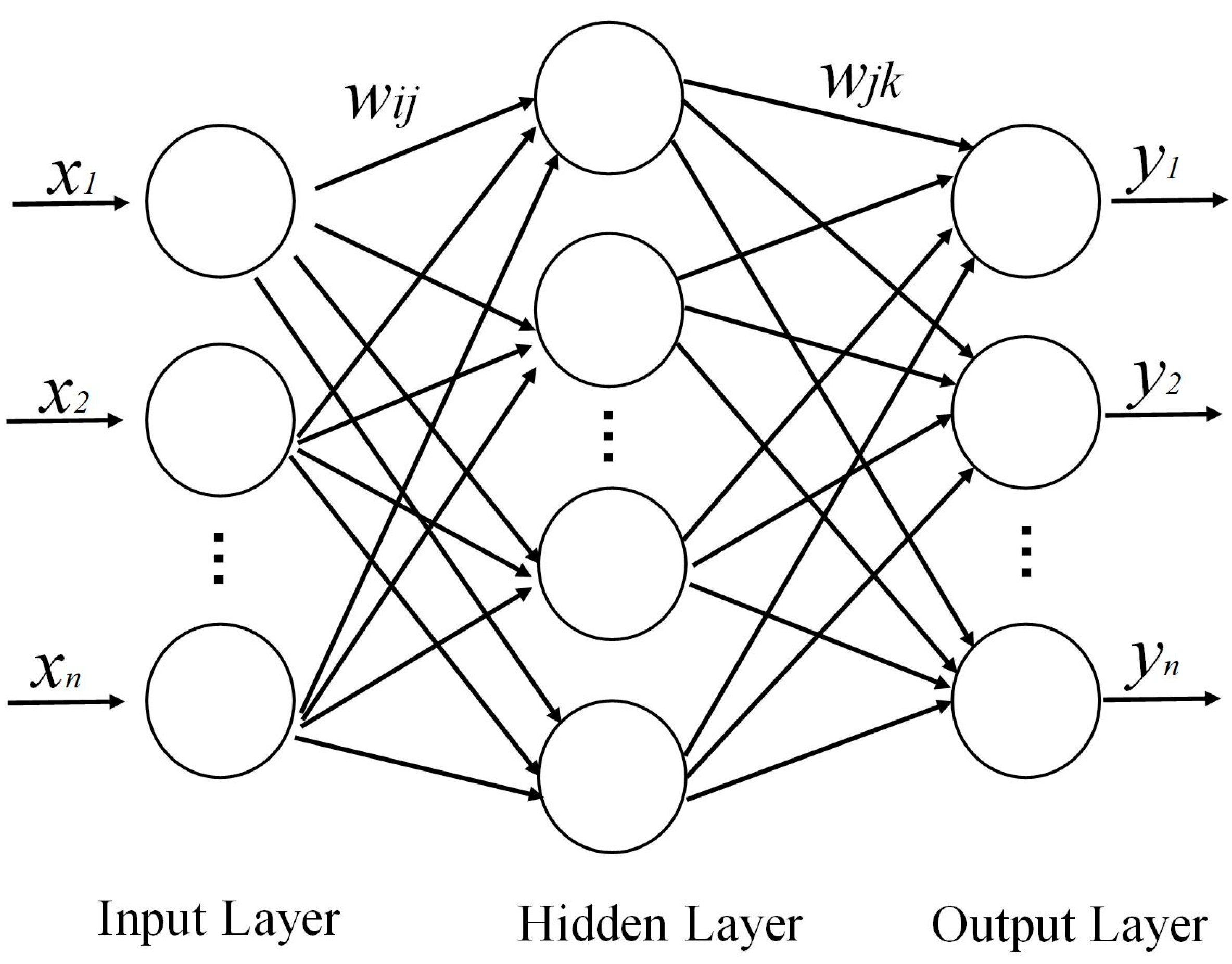
Figure 1. The structure of BP neural network.
Mathematics 10 01746 g001
Figure 2. The structure of mind evolutionary computing.
Mathematics 10 01746 g002
Figure 3. Flow chart of numerical analysis and sample establishment.
Mathematics 10 01746 g003
Figure 4. The flow chart of the MEA-BP prediction model.
Mathematics 10 01746 g004
Figure 5. The monitoring points of roadway deformation.
Mathematics 10 01746 g005
Figure 6. Laser range finder.
Mathematics 10 01746 g006
Figure 7. Three-dimensional numerical analysis model.
Mathematics 10 01746 g007
Figure 8. Importance analysis results of input variables.
Mathematics 10 01746 g008
Figure 9. The variation of RMSE for three predicted variables.
Mathematics 10 01746 g009
Figure 10. Comparison between the BP model and MEA-BP model. (a) Elastic modulus. (b) Cohesion. (c) Friction angle.
Mathematics 10 01746 g010
Figure 11. Comparison of surrounding rock deformation results. (a) the displacement of ∆A. (b) the displacement of ∆D. (c) the displacement of ∆BC.
Mathematics 10 01746 g011
Table 1. Physical and mechanical parameters of surrounding rock.
Mechanical ParametersDensity
ρ/Kg·m−3
Elasticity Modulus E/GPaPoisson’s Ratio/μCohesion
c/MPa
Friction Angle φ/(°)Dilation Angle
ψ/(°)
Value24503~13.50.210.5~415~32.510
Table 2. Rock mechanical parameters and levels for orthogonal experimental.
LevelParameter
E/MPac/MPaφ
130.515
24.51.017.5
36.01.520
47.52.022.5
59.02.525
610.53.027.5
712.03.530
813.54.032.5
Table 3. The rock mechanical parameter and deformation for test samples.
GroupMechanical ParametersDisplacement/mm
E/MPac/MPaφ∆A∆D∆BC
112.692.4924.08−19.316.9−20.6
29.912.2529.92−18.321.015.0
33.011.8625.28−93.479.1−126.0
43.840.7832.10−82.282.7−115.8
57.252.2416.40−65.741.8−110.7
64.010.6331.15−102.797.8−143.0
76.761.8236.40−24.229.9−14.7
86.342.5417.38−55.136.3−87.5
Table 4. The RMSE for three input variables.
No.RMSE1RMSE2RMSE3RMSE*
16.047.603.670.93
24.661.495.131.20
31.718.251.630.31
46.4110.621.350.49
50.351.650.580.48
65.1610.074.600.24
72.672.092.880.40
82.013.450.860.57
Average3.635.652.590.58
Table 5. Parameters of two prediction models.
Prediction ModelThe Initial Values
BP modelη = 0.05; g = 0.001
MEA-BP modelη = 0.05; S = 200; m = 10; Nt = 5; Ns = 5; g = 0.001
Table 6. The deformation and predicted mechanical parameters of roadway.
Measuring PointRoadway Deformation ValuePredicted Mechanical Parameter
∆A/mm∆D/mm∆BC/mmE/MPac/MPaφ
1-1−60.941.4−96.18.522.2315.79
1-2−64.841.2−108.98.032.1815.84
2-1−90.778.5−96.43.161.7626.27
2-2−83.975.5−91.53.301.7226.98
Publisher’s Note: MDPI stays neutral with regard to jurisdictional claims in published maps and institutional affiliations.