
Tell Me Why I Do Not Like Mondays

School of Business, Faculty of Social Sciences, University of Haifa, Haifa 3498838, Israel
*
Author to whom correspondence should be addressed.
Mathematics 2022, 10(11), 1850; https://doi.org/10.3390/math10111850
Submission received: 5 May 2022
/
Revised: 24 May 2022
/
Accepted: 25 May 2022
/
Published: 27 May 2022
(This article belongs to the Special Issue Mathematical Aspects of Trading and Valuating Financial Assets)
Abstract
:We conduct a strict and broad analysis of the 30-day expected volatility (VIX) of five very active individual US stocks, three US domestic indices, and that of 10-year US Treasury notes. We find prominent non-random movement patterns mainly on Mondays and Fridays. Furthermore, significant leaps in expected volatility on Monday occur primarily in the first two and the fifth Mondays of the month. We also document that higher values for the 30-day expected volatility on Mondays are more likely when there was a negative change in the volatility on the preceding Fridays. This pattern does not occur on other subsequent days of the week. The results are robust through time and different subsamples and are not triggered by outliers or the week during which the options on the underlying assets expire. Rational and irrational drivers are suggested to explain the findings. Given that, to date, no one has conducted such an examination, our findings are important for investors interested in buying or selling volatility instruments.
JEL:
G12; G13; G14; G32MSC:
91-11“Tell me why
I don’t like Mondays
I want to shoot the whole day down…”
(The Boomtown Rats, The Fine Art of Surfacing, 1979)
https://www.youtube.com/watch?v=-Kobdb37Cwc (accessed on 5 May 2022).
1. Introduction
The empirical finance research has documented the day-of-the-week effect not only in equities [1,2], but also in commodities (e.g., [3,4]), currencies (e.g., [5]), cryptocurrencies (e.g., [6,7]), Treasury bills (e.g., [8]), and corporate bonds (e.g., [9]). These studies maintain that Monday returns are significantly lower than those of other weekdays, and Friday returns are significantly positive or the highest.
In this study, we extend the literature by showing that the well-known Monday effect also occurs in the expected 30-day volatility (VIX) of five active individual stocks (Amazon, Apple, Goldman Sachs, Google, and IBM), three US domestic indices (the Dow Jones, Russell 2000, and NASDAQ), and the VIX of 10-year Treasury notes. As far as we know, the question of whether the perceived risk is higher on certain days of the week has not been addressed for these specific volatility vehicles.
Exploring cyclicality in the expected 30-day volatility of bonds and equities is important for the designing of volatility hedging strategies. Doing so is important to test the validity of the market efficiency hypothesis, particularly given that exchange volatility products have become a popular investment vehicle in recent years. In addition, the day-of-the-week anomaly has been under fire in the last two decades. Various studies have reported a lack of adequate support for this anomaly (e.g., [10,11]), inconsistencies in its permanence (e.g., [12]) and even contradictory results (e.g., [13]). Given this debate and the lack of research on the seasonality of market expectations about the looking-forward volatility of individual stocks and bonds in the next 30 days, we seek to fill this gap in the literature and resolve some of these issues.
We subjected our findings to a battery of robustness checks and found, for example, that among the 319 Mondays in the VIX-style estimate of the expected 30-day volatility of Treasury notes (for May 2013 to February 2020), there were 224 Mondays (70.22%) associated with a positive change, and among the 342 sampled Fridays, there were 219 cases (64%) of a negative change.
As the expiration of options might be a factor inducing liquidity and price effects in the underlying assets (e.g., [14]), we control this possibility by removing the week on which the options on our securities of interest expired from consideration. Nevertheless, the regularity explored here was still evident. A more in-depth analysis of the volatility indices’ levels indicates that the hike in the expected 30-day volatility of 10-year bonds, equity indices, and individual stocks is strongly evident on the first, second, and fifth Mondays of the month, but moderately so in the fourth week, leaving the third Monday of the month with no clear direction. Regardless of the sub-period analyzed, this result holds for the vast majority of volatility indices examined. For example, the first Monday of the month was positive in 75% of the cases for Amazon, and 80.56% for Google, whereas the fifth Monday was positive in 74.39% of the cases for Apple, 73.75% for Goldman Sachs, and 75.61% for the Russell 2000.
The results also indicate that the direction of the estimate of the expected 30-day volatility on Mondays is contingent on that of Fridays. The probability for a positive change in the VIX-style estimate on Monday is greater if the preceding Friday ended with a decline in the VIX. For example, a drop in the expected 30-day volatility on Fridays was followed by a positive change on Mondays for 74% of the cases in the Treasury notes (TYVIX), 61.5% of the cases in the Apple VIX (VXAPL), and 63.64% of the cases in the Russell 2000 VIX (RVX). Nevertheless, this Friday–Monday pattern does not occur on other subsequent days of the week.
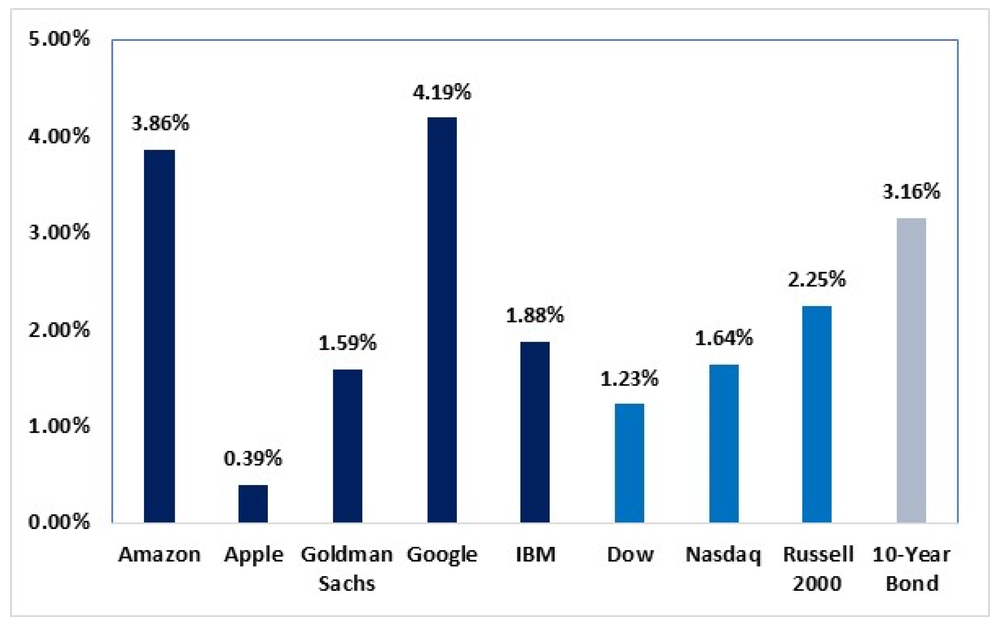
Practically, none of the indices examined here are tradable. However, if we assume that these indices are tracked precisely by ETNs or ETFs, then investors could benefit substantially from constructing simple trading rules that take advantage of the patterns documented here. Figure 1 illustrates the weekly excess returns resulting from the difference between the returns of the volatility index on Mondays and Fridays (). Pronounced returns can be obtained if investors short the volatility index on Thursday, buy it twice on Friday (the first acquisition is aimed at closing the short position, while the other is designed to take a new long position), and then sell it again on Monday. The average weekly profits are striking and range from 0.39% (for Apple) to 4.19% (for Google). These theoretical profits are still evident after accounting for reasonable levels of transaction costs and using different subsamples.
We suggest two different, if somewhat related, explanations for the results. The first is the variation in the type of economic news across the week. We observe that there is increased pessimism reflected in the press at the start of the week. Specifically, we find that the Economic Policy Uncertainty Index (EPU; [15]), an index developed using text analyses of US newspapers, is lower on Fridays but sharply higher on Sundays and Mondays. Figure 2 illustrates the average of the EPU index across weekdays.
In parallel, and as a complementary effect, there is a body of literature that relates the negative atmosphere on Monday to the timing of corporate news announcements. These studies, detailed in Section 2, maintain that companies tend to release good corporate news during trading hours and bad news on Friday after the market closes.
The second explanation (detailed in Section 2.2) relies on the irrational factor of investors’ moods. Prior lab-based, survey-based, and social media-based works from psychology, decision-making, social media, sleep, and transportation have established that people’s mood varies across weekdays, claiming that it improves on Fridays but sharply declines on Mondays (e.g., [16,17]). The psychology and decision-making literature have also established that mood affects people’s judgment and decision-making significantly, and that psychological state influences their attitude toward risk (e.g., [18]). Hence, emotional states are potentially capable of affecting investors’ risk assessments and preferences and, ultimately, their investment decisions. Indeed, many studies have documented that agents’ financial decisions do vary with investor mood [19,20] and that market volatility reacts to investor sentiment [21].
Methodologically, we suggest decomposing the volatility into two components. The first component reflects all of the fundamental or rational economic variables derived from daily and intraday (5 min) data, while the second reflects irrational factors (captured by the residuals). We find that the irrational component exhibits a non-random discrepancy across weekdays, with a significant leap on Monday and a decline on Friday. This finding confirms our premise that irrational factors might explain part of this phenomenon.
Our results confirm the claim that the 30-day expected volatility of bonds, equity indices, and individual stocks not only reflects the market participants’ views about future market volatility as expressed through trade, but also mirrors investors’ daily sentiment. Many studies have pointed to the VIX as an indicator of risk aversion and investors’ mood or sentiment (e.g., [22,23]), where a rise (decrease) in the VIX reflects increased (deteriorating) perceptions about risk aversion or fears. Overall, both the rational and irrational explanations are in line with the global pictures explored here.
2. Literature Review
2.1. Explanations Based on Investors’ Rational Considerations
The literature lists various possible rational explanations for the Monday anomaly: the high Friday return hypothesis (e.g., [24]), individual traders’ decision-making processes following recommendations from brokerage houses (e.g., [25,26,27,28,29]), asymmetric risk between long and short positions around weekends [30], and the correlation structure (long memory) of the series [31].
One explanation that has attracted a great deal of attention in the literature is the timing of corporate announcements. Ref. [32] noted that positive corporate news is more likely to be announced during trading hours. Furthermore, companies are more likely to release negative news at the close of trading on Friday rather than on other days. Ref. [33] documented that unanticipated negative earnings announcements are more likely on Monday or over the weekend than on other weekdays. Consistent with [33,34] maintained that on Friday, investors’ inattention is more likely. Hence, Fridays are associated with more delayed responses relative to other weekdays. Other studies corroborate this evidence (e.g., [35]). These studies maintain that managers strategically time their corporate announcements. Hence, bad news is more likely to be announced on Friday than on other weekdays, the day before a national holiday, when attention is limited, and after the market closes.
In addition to the tone of corporate announcements, previous papers have confirmed the role of the mass media and news coverage in affecting the price and volatility of asset prices and the formation of investors’ expectations about future stock values (e.g., [36]). Many studies apply textual analysis techniques to provide comprehensive evidence about the significant relationship between information coverage and trading volume, returns, and volatility. For example, [37] observed that when the media express a high degree of pessimism, investors react, often leading to a decline in market prices. In addition, [38] found that variations in a firm’s indicators of profitability and price efficiency are related to the percentage of negative words in the financial news.
In this spirit, [15] conducted textual analyses of newspaper texts to create a tool that would reflect economic and policy conditions. They reported that greater government policy uncertainty is associated with increased stock price volatility and less employment and investment in economic sectors such as defence, health care, finance, and infrastructure construction. In this spirit, recent studies confirm that fiscal pressure and financial solvency are capable of affecting the performance of public companies [39,40,41].
2.2. Explanations Based on Investors’ Irrationality
The conventional framework of the finance theory implies that irrational factors do not play any role in influencing asset prices. However, the behavioural approach maintains that investor moods—reflected in optimistic or pessimistic expectations—can persist and affect asset prices for significant periods. Evidence in the behavioural finance literature shows that stock returns are associated with people’s moods. In these studies, mood is captured using variations in natural conditions such as the weather (e.g., [42]) and amount of daylight (e.g., [43]). These studies are based on psychology and maintain that mood influences people’s attitude toward risk. Consequently, returns on securities fluctuate with investors’ moods.
Several works justify the lower returns on Mondays using the notion of mood. These studies maintain that people’s mood does not randomly fluctuate across weekdays. Rather, it peaks on the weekend and slides sharply on Monday. For example, [44] explored the existence of the Blue Monday syndrome and maintained that when investors are feeling down, they are more pessimistic about the outlook for the securities they hold and more apt to sell for less on Mondays than on other days. In this spirit, [4] utilized indirect proxies previously used in the literature to proxy for mood, including US closed-end fund discounts, returns on small stocks, consumer confidence and consumer attitudes towards buying a house. They argued that the Monday effect is more evident during periods of pessimism, implying that irrationality on the part of investors may explain the higher non-diversifiable risk on Mondays.
In many survey-based studies, Monday is viewed as the worst morning of the week (e.g., [16]). People who are asked why they do not like Mondays almost always point to the following themes. Generally, they talk about the difficulty of waking up on Monday after the weekend. Even those who say they had a full night’s sleep often describe being tired on Monday [45]. Others cite the extra traffic on Mondays when commuting, noting that Mondays are the most congested mornings of the week [46,47]. The stress involved in arriving late to work also affects financial decision-making (e.g., [48] provide a comprehensive review). In addition, people claim that Monday marks the move from the leisure activities of the weekend to the beginning of five long workdays [44]. Studies on suicide document that Mondays are the peak days for suicides (e.g., [49]), with significantly fewer suicides on weekends [50]. All of these factors could play a role in fluctuations in investors’ moods, which could affect their attitude toward risk.
Admittedly, it is hard to assess mood outside the lab using real-life data. However, ref. [51] suggested capturing the collective mood using data from social media. The authors examined data from about 509 million Twitter posts by 2.4 million users from numerous countries with differences in religion and culture. They documented that people tend to be more positive on weekends and early in the morning, and less on Mondays. Similar results are also reported in other studies (e.g., [52,53]). Ref. [54] showed that investors’ moods, captured by Facebook status updates, deteriorate on Mondays, mainly for small capitalization indices and countries in which there is a greater desire to avoid uncertainty.
3. Data
To explore the role of these various factors in investors’ decisions, we use daily data about the expected 30-day volatility of five very active individual stocks: Amazon, Apple, Goldman Sachs, Google, and IBM. Our data come from the Chicago Board Options Exchange (CBOE) website. At this stage, the only individual stocks for which the CBOE computes its VIX are those used here. We also used data about the VIX-style estimate of the expected 30-day volatility of the Dow Jones (VXD), NASDAQ (VXN), and Russell 2000 (RVX) and used data about the expected volatility of 10-year Treasury notes (TYVIX). Finally, we utilized 5 min data obtained from pitrading.com to construct estimates of realized variances for the assets explored here. Table 1 describes the sample periods considered, the number of observations, and the source of the data. The longest sample for equity market indexes is that of the VXN (October 2000 to February 2020), and the shortest one is that of the VXD (October 2013 to February 2020).
Table 2 presents the descriptive statistics of the VIX. Panel A of the table reports the statistics of the data in level, while Panel B reports the correlation between the volatility measures. For example, according to Panel A, the expected volatility of Amazon (VXAZN) spans August 2011 to February 2020, and the total number of observations was 2148. The average value of the level VIX was 31.69%, and its standard deviation was 8.63%. During the sample period, the VIX leapt to 66.06% during the subprime crisis, and the lowest value was 5.13%. Panel C of the table reports the average rate of return in the expected 30-day volatility across weekdays for the sampled securities. In this panel, we present the results of testing three different hypotheses:
- (1)
- The first conjectures that the implied volatility is equal across weekdays. Based on the findings, we rejected this hypothesis for all of the sampled securities, as evident by the significant F-statistic values.
- (2)
- The second hypothesis postulates that changes in the VIX are equal on Monday and Friday. Based on the findings, we rejected this hypothesis as well.
- (3)
- Last, we checked whether the mean returns on the VIX are equal on Monday, Tuesday, Wednesday, and Thursday.
Based on the findings, we rejected this hypothesis, as evident by the F-statistic values in the right column of Panel C of Table 2. Therefore, there was no support for any of the hypotheses about equality across weekdays or equality between Mondays and Fridays.

Table 2.
Descriptive statistics.
| Panel A: Level Data in (%). | |||||||||||
| VXAZN | VXAPL | VXGSCLS | VXGOG | VXIBM | VXD | VXN | RVX | TYVIX | |||
| Mean | 31.69 a | 28.00 a | 26.92 a | 24.61 a | 21.84 a | 14.82 a | 25.28 a | 20.13 a | 4.98 a | ||
| Med. | 29.86 | 27.33 | 25.34 | 23.86 | 20.63 | 13.93 | 20.01 | 18.56 | 4.93 | ||
| Max. | 66.06 | 62.60 | 74.88 | 55.60 | 51.72 | 42.67 | 83.00 | 57.66 | 8.62 | ||
| Min. | 5.13 | 12.52 | 16.16 | 9.21 | 13.23 | 7.58 | 10.31 | 11.83 | 3.16 | ||
| Stdev. | 8.63 | 6.55 | 7.57 | 6.20 | 4.96 | 3.72 | 13.76 | 6.01 | 0.95 | ||
| Skew. | 0.66 | 0.84 | 2.13 | 0.89 | 1.23 | 1.68 | 1.83 | 2.53 | 0.66 | ||
| Kurt. | 3.19 | 4.15 | 9.63 | 4.13 | 5.29 | 7.76 | 5.85 | 10.96 | 3.42 | ||
| #Obs | 2148 | 2148 | 2112 | 2148 | 2148 | 1602 | 4825 | 2149 | 1697 | ||
| Sample Period | 2011:08 to 2020:02 | 2011:08 to 2020:02 | 2011:10 to 2020:02 | 2011:08 to 2020:02 | 2011:08 to 2020:02 | 2013:10 to 2020:02 | 2000:10 to 2020:02 | 2011:08 to 2020:02 | 2013:05 to 2020:02 | ||
| Panel B: Correlation between the Volatility Measures. | |||||||||||
| VXD | VXN | RVX | TYVIX | VXAZN | VXAPL | VXGSCLS | VXGOG | VXIBM | |||
| VXN | 0.95 *** | 1.00 | |||||||||
| [124.97] | ----- | ||||||||||
| RVX | 0.96 *** | 0.90 *** | 1.00 | ||||||||
| [138.11] | [86.49] | ----- | |||||||||
| TYVIX | 0.53 *** | 0.46 *** | 0.60 *** | 1.00 | |||||||
| [25.85] | [21.25] | [31.11] | ----- | ||||||||
| VXAZN | 0.62 *** | 0.65 *** | 0.61 *** | 0.33 *** | 1.00 | ||||||
| [32.25] | [35.63] | [31.39] | [14.20] | ----- | |||||||
| VXAPL | 0.84 *** | 0.83 *** | 0.81 *** | 0.51 *** | 0.75 *** | 1.00 | |||||
| [63.81] | [62.29] | [57.09] | [24.58] | [46.21] | ----- | ||||||
| VXGSCLS | 0.92 *** | 0.90 *** | 0.93 *** | 0.58 *** | 0.56 *** | 0.80 *** | 1.00 | ||||
| [99.52] | [85.59] | [102.22] | [29.18] | [27.88] | [55.56] | ----- | |||||
| VXGOG | 0.81 *** | 0.83 *** | 0.78 *** | 0.41 *** | 0.85 *** | 0.86 *** | 0.77 *** | 1.00 | |||
| [56.07] | [61.17] | [51.75] | [18.80] | [67.45] | [68.91] | [49.67] | ----- | ||||
| VXIBM | 0.86 *** | 0.86 *** | 0.84 *** | 0.43 *** | 0.61 *** | 0.80 *** | 0.89 *** | 0.80 *** | 1.00 | ||
| [70.39] | [70.00] | [62.95] | [19.82] | [32.07] | [54.84] | [81.31] | [54.73] | ----- | |||
| Panel C: Rate of Change in Volatility across Weekdays. | |||||||||||
| Mon () | TUE () | WED () | THU () | FRI () | H0: α2= α3= α4= α5= α6 | H0: α2= α6 | H0: α2=α3= α4= α5 | ||||
| VXAZN | 2.228 a | 0.619 c | 0.419 | 0.839 b | −2.549 a | 26.54 a | 9.87 a | 5.65 a | |||
| (6.39) | (1.85) | (1.25) | (2.49) | (−7.59) | |||||||
| VXAPL | 1.264 a | −0.245 | −1.255 a | 0.335 | 0.146 | 7.36 a | 2.33 b | 9.76 a | |||
| (3.65) | (−0.74) | (−3.79) | (1.01) | (0.44) | |||||||
| VXGSCLS | 1.243 a | −0.149 | −0.133 | −0.026 | −0.888 a | 6.45 a | 4.99 a | 4.93 a | |||
| (4.04) | (−0.51) | (−0.45) | (−0.09) | (−2.99) | |||||||
| VXGOG | 2.626 a | 0.345 | 0.158 | 0.66 c | −2.167 a | 24.18 a | 9.75 a | 10.55 a | |||
| (7.41) | (1.02) | (0.47) | (1.94) | (−6.35) | |||||||
| VXIBM | 1.599 a | 0.262 | −0.832 b | 0.049 | −0.822 b | 7.99 a | 4.86 a | 8.14 a | |||
| (4.46) | (0.76) | (−2.42) | (0.14) | (−2.38) | |||||||
| VXD | 1.596 a | 0.657 | −0.644 | 0.589 | −0.527 | 5.13 a | 3.64 a | 5.03 a | |||
| (3.81) | (1.63) | (−1.60) | (1.45) | (−1.30) | |||||||
| VXN | 1.678 a | 0.009 | −0.243 | 0.06 | −0.571 a | 19.18 a | 8.06 a | 19.57 a | |||
| (8.36) | (0.05) | (−1.26) | (0.31) | (−2.9) | |||||||
| RVX | 1.944 a | 0.259 | −0.143 | −0.118 | −0.855 a | 11.85 a | 6.56 a | 10.59 a | |||
| (6.32) | (0.88) | (−0.49) | (−0.39) | (−2.89) | |||||||
| TYVIX | 2.039 a | 0.403 | −0.740 a | −0.214 | −1.288 a | 24.74 a | 9.16 a | 21.89 a | |||
| (7.80) | (1.61) | (−2.95) | (−0.85) | (−5.10) | |||||||
Notes: Panel A of the table reports the descriptive statistics of the looking-forward volatility variables. “a” denotes statistical significance at the level of 1%. The squared parentheses in Panel B report the T-Statistic values. “***” denotes statistical significance at the 1% level. Simple average values of the returns across weekdays. The values in parentheses are the t-stat. values, while “a,” “b”, and “c” denote statistical significance at the levels 1%, 5%, and 10%, respectively. The values reported on the right-hand side of the table are the F-statistic values for three different hypotheses. Overall, the hypothesis for equality across weekdays and equality between Monday and Friday are rejected. The model used is as follows. ; is the rate of change in the price of the volatility index. MON, TUE, WED, THU, and FRI are dummy variables that capture the day of the week. The T-Statistics are Newey–West [57] corrected.
4. Empirical Findings
Table 3 summarizes the distribution of the expected 30-day volatility indices on Fridays and Mondays. As outliers in the data could potentially yield biased inferences [58], we utilized the sign test. The test is free from the effect of outliers and validates whether the resulting ratio is statistically different from 0.5—the probability of a coin toss. The picture that emerges indicates that Fridays are associated with a decrease in the expected 30-day volatility, and that Mondays are associated with a positive increase in it. This finding holds true for the VIX of the individual stocks, indices, and Treasury notes. For example, regarding the VXAZN data, the table indicates that out of the 434 Fridays, there were 276 Fridays associated with a decrease in the VIX. In other words, 63.59% of the Fridays were associated with a negative change. In parallel, among the 402 Mondays, there were 261 cases of a positive change in the VIX—yielding 64.93% positive Mondays. The difference between the percentage of times there was a decline on Friday and an advance on Friday (63.59–35.94% = 27.65%) was strongly significant (t-stat. = 8.47). In addition, the difference between the percentage of times there was an increase on Monday and a decline on Monday (64.93–35.07% = 29.85%) was strongly significant as well (t-stat. = 8.86).
A similar picture emerges for the rest of the US single stocks. The percentages of negative Fridays in the rest of the domestic US indices were as follows: VXAPL (53.69%), VXGSCLS (63%), VXGOG (63.36%), VXIBM (55.53%). As the sign test indicates, all of these percentages are significantly and statistically different from 50%. In each panel of Table 3, we report the mean and median returns on Fridays and Mondays.
The percentage of negative Fridays in the VIX-style measure of other domestic US indices was 60.68% for the Dow’s VXD, 61.92% for the NASDAQ’s VXN, and 59.91% for the Russell 2000′s RVX. On the other hand, the percentage of positive Mondays exhibits a similar pattern for the Dow (57.62%), NASDAQ (59.10%) and Russell 2000 (60.05%). These results refute the hypothesis that the percentage equals 50%, indicating a high degree of systematic patterns. Lastly, the percentage of negative Fridays in the VIX of the Treasury notes (TYVIX) was 64.04%. On the other hand, the percentage of positive Mondays in the TYVIX was 70.22%.
The expiration of options might be a factor promoting liquidity and price effects in the underlying assets (e.g., [59]). To eliminate this possibility, we removed the week on which the options on our securities of interest expired from consideration. We repeated the tests that appear in Table 3 (According to the CBOE, the standard expiration date for equity indices, stocks, ETNs, and ETFs occurs on the third Friday each month). The results, reported in Table 4, are qualitatively unchanged. Indeed, we saw a tendency for the phenomenon to intensify.
Table 5 (and Table S1 in Supplementary Materials) provides a more detailed picture of the Monday effect, categorized by the week of the month. Given that some months include five Mondays, we followed [60] in defining the first week of the month as that containing the first trading day of the month. If Monday is the first trading day of the month, we consider it the start of the first week of the month. Otherwise, there is no Monday return for the first week of the month. “***”, “**”, and “*” indicate the statistical significance at the 1%, 5%, and 10% levels, respectively.
The table tracks the 30-day volatility returns obtained on each Monday of the month, and reports the means, t-statistics, Welch F-statistics, ratio of positive returns, and number of observations. The “all weeks” column in the table reports the aggregated Monday returns. This column is positive in all cases regardless of the security and time period selected. Categorizing the Monday returns by the week of the month provides more finely grained distinctions in the returns. The first, second, and fifth Mondays of the month were associated with statistically significant positive returns, and the percentage of positive returns was quite high. For example, the first week Monday was positive in 75% of the cases for Amazon, 72.22% for Apple, 57.14% for Goldman Sachs, 80.56% for Google, and 72.22% for IBM. The fifth Monday was also positive in 65.85% of the cases for Amazon, 74.39% for Apple, 73.75% for Goldman Sachs, 73.17% for Google, and 78.05% for IBM. Very similar significant results were also evident for the equity and bond volatility indices: 69.35% for the VIX of the Dow Jones Index (VXD), 70.05% for the NASDAQ volatility index (VXN), 75.61% for the Russell 2000 (RVX), and 67.69% for the 10-year Treasury notes (TYVIX).
The Mondays of the fourth week were positive and statistically significant in five out of the nine indices considered. In contrast to the results obtained above, the Mondays of the third week had insignificant returns. Indeed, when considering the full sample, they even tended to be negative in five out of the nine volatility indices.
We combined the Monday returns of the first three weeks and compared the outcome (reported in the “first three weeks” column) with that resulting from combining the Monday returns of the last two weeks of the month (the fourth and fifth weeks reported in “last two weeks” column). The difference between these two Monday combinations was positive in eight out of the nine indices examined. However, only in three cases—Amazon, Google, and the RVX—was the difference statistically significant.
Overall, these findings indicate that the expected 30-day volatility of bonds, equity indices, and individual stocks is largely driven by the first, second, and fifth Mondays of the month and moderately by the fourth week. For robustness, we separated the sample into two relatively equal subsamples. The results remained essentially the same. These findings make the roots of this pattern difficult to explain based on rational factors, particularly given that the week on which the options expire is not the catalyst behind this anomaly.
In Table 6 (and Table S2 in Supplementary Materials), we conduct the same procedure and categorize Fridays by the week of the month in order to track the 30-day volatility returns obtained on each Friday of the month. Except for the VXD, the first, second, and third Fridays of the month are associated with negative returns, and the percentage of negative returns is quite high. For example, the first week Friday is negative in 68.3% of the cases for Amazon, 63.4% for Apple, 72.5% for Goldman Sachs, 68.3% for Google, and 63.4% for IBM. Similar significant results were also obtained in the equity and bond volatility indices: 67.7% for the NASDAQ volatility index (VXN), 68.3% for the Russell 2000 (RVX), and 76.7% for the 10-year Treasury notes (TYVIX).
We combined the Friday returns of the first three weeks and compared the outcome (reported in the “first three weeks” column) with that resulting from combining the Friday returns of the last two weeks of the month (the fourth and fifth weeks reported in “last two weeks” column). The difference between these two Friday combinations was negative in eight out of the nine indices examined, meaning that the expected 30-day volatility of bonds, equity indices, and individual stocks is largely driven by the first, second, and third Fridays of the month.
Table 6.
Summary statistics for the Friday return categorized by week.
| Panel A: Amazon. | |||||||||
|---|---|---|---|---|---|---|---|---|---|
| First Friday | Second Friday | Third Friday | Fourth Friday | Fifth Friday | First Three Fridays | Last Two Fridays | Difference in the Two Periods | All Fridays | |
| 1.08/2011–02/2020 | |||||||||
| Mean | −3.066 a | −0.913 | −1.314 a | −1.471 | −6.684 a | −1.445 a | −3.942 a | −2.549 | |
| T-Statistic | (−3.13) | (−1.64) | (−2.88) | (−1.64) | (−5.06) | (−4.21) | (−4.90) | −2.497 a | (−6.25) |
| Welch F-test | (−2.84) | ||||||||
| Percentage negative | 68.29% | 72.00% | 64.36% | 55.45% | 60.44% | 68.18% | 57.81% | (−2.70) | 63.59% |
| #Obs | 41 | 100 | 101 | 101 | 91 | 242 | 192 | 434 | |
| 2.08/2011–12/2015 | |||||||||
| Mean | −1.704 c | −1.458 a | −0.827 | −3.096 b | −6.127 a | −1.225 a | −4.551 a | −2.730 a | |
| T-Statistic | (−1.89) | (−2.92) | (−1.34) | (−2.05) | (−3.52) | (−3.38) | (−3.95) | −3.326 a | (−4.81) |
| Welch F-test | (−2.89) | ||||||||
| Percentage negative | 68.42% | 74.00% | 61.54% | 61.54% | 60.42% | 67.77% | 61.00% | (−2.75) | 64.71% |
| #Obs | 19 | 50 | 52 | 52 | 48 | 121 | 100 | 221 | |
| 3.01/2016–02/2020 | |||||||||
| Mean | −4.243 b | −0.367 | −1.830 a | 0.254 | −7.306 a | −1.664 a | −3.279 a | 1.943 b | |
| T-Statistic | (−2.59) | (−0.37) | (−2.73) | -0.29 | (−3.60) | (−2.85) | (−2.93) | −1.615 | −2.51 |
| Welch F-test | (−1.18) | ||||||||
| Percentage negative | 68.18% | 70.00% | 67.35% | 48.98% | 60.47% | 68.60% | 54.35% | (−1.07) | 62.44% |
| #Obs | 22 | 50 | 49 | 49 | 43 | 121 | 92 | 213 | |
Notes: The table reports the average daily return of the volatility index on each Friday of the month. Friday may appear five times in a certain month. If the first trading day of the month occurs on Friday, we will have five Fridays in that month. If the first trading day of the month is other than Friday, then no Friday is attributed to the first week of the month. The “first three weeks” column reports the average of returns on the first three Fridays combined. The “last two weeks” column reports the average returns of the fourth and fifth Fridays combined. “a,” “b”, and “c” indicate the regular levels of statistical significance. Table S2 reports the test results for the rest of the volatility measures.
We also examined the performance of the 30-day expected volatility using year-by-year snapshots and computed the ratios of the positive Fridays and Mondays for each of the sampled securities. Table S3 in Supplementary Materials summarizes the results for the sampled indices. In addition, further robustness checks regarding the sign direction of Fridays and Mondays (with two equal subsamples) appear in Table S4 in Supplementary Materials.
Overall, the results are consistent over time and across the different sampled securities. They indicate that the VIX-style volatility indices performed better on Mondays (column “+Monday”) than on Fridays (column “+Friday”) in terms of the percentage of times the index advanced, the mean percentage change (fifth column vs. fourth column), and the median percentage change in each year of this period (the last two columns). Generally, the results contradict the conclusions drawn by prior works maintaining that, according to the efficient market hypothesis, once a pricing inefficiency becomes known to the public, it will vanish [61]. Specifically, [62] claimed that the seasonal effects documented in the finance literature often seem to reverse, diminish, or simply disappear post-academic publication.
4.1. Do Monday’s Price Changes Depend on Friday’s Price Changes?
Table 7 depicts the performance of the expected 30-day volatility measure (the VIX) on Monday, contingent on the change in the VIX on the preceding Friday. For example, the picture obtained for the VIX-style estimate for Apple (VXAPL) indicates that of the 183 times in which there was a positive change in the VIX on Friday, there was a subsequent positive change on Monday in 56.28% of the times (103 Mondays). However, of the 205 in which Fridays witnessed a negative change in the VIX, there were 126 subsequent Mondays with a positive change in the VIX, meaning 61.46% of the time. The largest ratio occurs for the VIX-style measure of the 10-year Treasury notes. As Table 7 indicates, of the 197 in which Fridays witnessed a negative change in the price of the volatility index, there were 146 subsequent Mondays with a positive change in the price, meaning 74.11% of the time. The collective picture indicates that the probability of the volatility index returns being positive on Mondays () is greater when the preceding Fridays are associated with a negative change in the price. In other words, .
Regarding the VIX-style measure for Apple (VXAPL), the difference between the percentage of times there was an advance in the VIX on Monday after a decline on Friday and the percentage of times there was a decline in the VIX on Monday after a decline on Friday (61.46–38.54% = 22.93%) was strongly significant (t-stat. = 4.49). In parallel, the difference between the percentage of times there was an advance in the VIX on Monday after an advance on Friday and the percentage of times there was a decline in the VIX on Monday after an advance on Friday (56.28–43.17% = 13.11%) was significant as well (t-stat. = 2.43). Similar results were obtained with respect to other individual stocks. For example, for the VXGOG, if Fridays are associated with a decline in the VIX, they are followed by a positive leap in the VIX in 68.27% of the cases.
In order to ensure that our findings above are free of outliers, we re-ran the test on a yearly basis. In Table S5 in Supplementary Materials, we summarize the results of this strict examination. Once again, we find that the percentage of Mondays on which there was an advance in the VIX was greater after a decline on Friday than after an advance on Friday. For example, this pattern was evident in the VXAPL in six out of the nine years. The mean change in the VIX on those Mondays preceded by a rise on Friday was 0.67%, whereas the mean change on those Mondays preceded by a decline on Friday was 0.90%. The corresponding median values were 1.12% and 1.03%, respectively. Overall, the probability of having an increase in the VIX on Monday is contingent on what happened on Friday.
4.2. A Comparison of Monday and Other Days of the Week
The relationship between changes in the VIX-style indices on Monday and on Friday is significantly different from the relationship between price changes on other successive business days. Table 8 shows how the VIX of the sampled securities performed on Monday and on days other than Monday, contingent on the direction of change the previous day.
As the table indicates, the percentage of time the VIX advanced after an increase on the previous day is greater on Monday than on days other than Monday. For example, after a positive change in the VXAZN on the previous day, there was a further positive change in the VIX on days other than Monday 47.52% of the time, in contrast to 67.36% on Mondays. The mean change in the VIX on days other than Mondays preceded by a rise on the previous day was −0.38%, whereas the mean change on those days preceded by a decline on the previous day was 0.10%.
Table 8 also summarizes the percentage of time the index advanced after a decline on the previous day, on Monday and on days other than Monday. The picture that emerges indicates that for days other than Monday, a decline in the VIX on day “t” is followed by an advance in the VIX in 48.66% of the cases. However, a decline in the VIX on Friday was followed by an advance in the index in 61.79% of the cases. Overall, the percentage of time the index advanced on Monday was higher than on days other than Monday for all indices in the sample.
The seasonality explored here accords with prior works assuming, implicitly, that seasonality effects are relatively stable across time. Not surprisingly, calendar effects are generally labelled using the relevant season: “Sell in May and go away”, the “holiday” effect, or the “Monday” effect. However, our findings contradict those of [63]. The authors used data for 11 equity markets and rejected the classic argument regarding the stability of the day-of-the-week effect.
4.3. Potential Drivers
4.3.1. Investors’ Irrationality
Level of mood or emotion is difficult to assess. Social science studies often use questionnaires or surveys for this purpose. However, given that we are interested in exploring the variation in investor mood across weekdays, we followed the literature and utilized the Twitter Happiness Index. The Twitter index is widely used in recent behavioural studies to reflect mood (e.g., [64]). Data about the Twitter Happiness Index are available from September 9, 2008. Table 9 reports the average daily values of the Twitter Happiness Index for the entire sample as follows: 6.011 (Monday), 6.009 (Tuesday), 6.010 (Wednesday), 6.015 (Thursday), 6.031 (Friday), 6.034 (Saturday–the highest) and 6.024 (Sunday). Statistical tests examining equality between the happiness values on Friday and Monday led us to reject this hypothesis (t-statistic = 7.51). In parallel, we do not reject the hypothesis that the happiness values on Monday equal those on Tuesday. These observations are in line with [52,65]. Both studies maintain that participants’ mood on Monday is not significantly different from that observed on Tuesday. Overall, our results accord with previous studies that evaluated individuals’ moods using questionnaires and surveys; the weekend is often associated with high values of happiness relative to Mondays, confirming that mood varies across weekdays.
Another way to explore non-rationality in pricing volatility is to examine whether they are rationally priced across weekdays. The level of a volatility index, which is an observed variable, is assumed to track the expected volatility of the underlying security, which can be an individual stock, a bond, or a market index. Recall that the level of any volatility index is calculated by the same procedure used in evaluating the VIX of the S&P 500 index.
We suggest decomposing the price of the volatility index (Vt) into two components. The first component reflects all of the fundamental or rational economic variables (VR), while the second reflects irrational factors (VIR). In other words,
This separation allows us to better understand the dynamic factors affecting the level of the volatility index. Thus, if irrational disturbances are absent, the observed price is said to completely reflect the economic value of the index. In other words,
where X is a matrix of potential rational fundamentals that are revealed in the underlying index. For the sake of robustness, we use the following stationary model that utilizes the first difference (i.e., rate of change).
denotes the rate of change in the volatility index. Ri,t denotes the rate of change in the price of the underlying index for security “i.” Similar to [66], we use contemporaneous as well as lagged returns of the underlying asset price and additional lagged changes in volatility to explain the current changes in the index price. H and K are set according to the Akaike and Hannan–Quinn information criteria and range between 1 and 3. RV is the actual (ex-post) realization of return variation for each security computed using 5 min data over the next 22 days, as suggested in [67]. We validated the stationarity of the variables using the augmented Dickey–Fuller test [68].
Once Equation (3) is estimated, we can compute the residuals of the model using . The residuals are designed to capture what rational factors cannot explain. Thus, they reflect the irrational component in the volatility price. The underlying assumption is that if the volatility index is rationally priced, the residuals should be the same for each trading day across the week. However, if the residuals originated in the spread between the VIX estimate and the ex-post realized volatility, and other related variables follow day-of-the-week patterns, then this would suggest that investors are making systematic pricing errors when predicting future volatility. Formally, the following regression model tests this proposition.
where Dayd is a dummy variable that captures the day of the week on which the return on the volatility index is observed. captures the expected residual on Dayd where d = 2, …, 6.
The estimation results of this model are presented in Table 10. A quick glance at the table shows that (average of residuals on Monday) was positive and statistically significant in all cases. In parallel, (average of residuals on Friday) was negative and statistically significant in the vast majority of cases. While the reported estimates for and were significantly different from zero, the rest of the coefficient estimates for through were very close to zero in most cases. The F-tests hypothesizing equality in these coefficients are jointly strongly rejected, indicating that the residuals behave in a non-random way across weekdays. Finally, the inclusion of other explanatory variables in Equation (3), such as the Treasury yield spread, corporate default spread, changes in gold prices, and inflation, did not change the results qualitatively. To save space, we do not present the estimation results, but they are available upon request. Overall, these findings support the premise that one of the driving forces in pricing volatility is the irrationality of investors, as evident in the positive and negative residuals on Monday and Friday, respectively.
4.3.2. Investors’ Rational Considerations
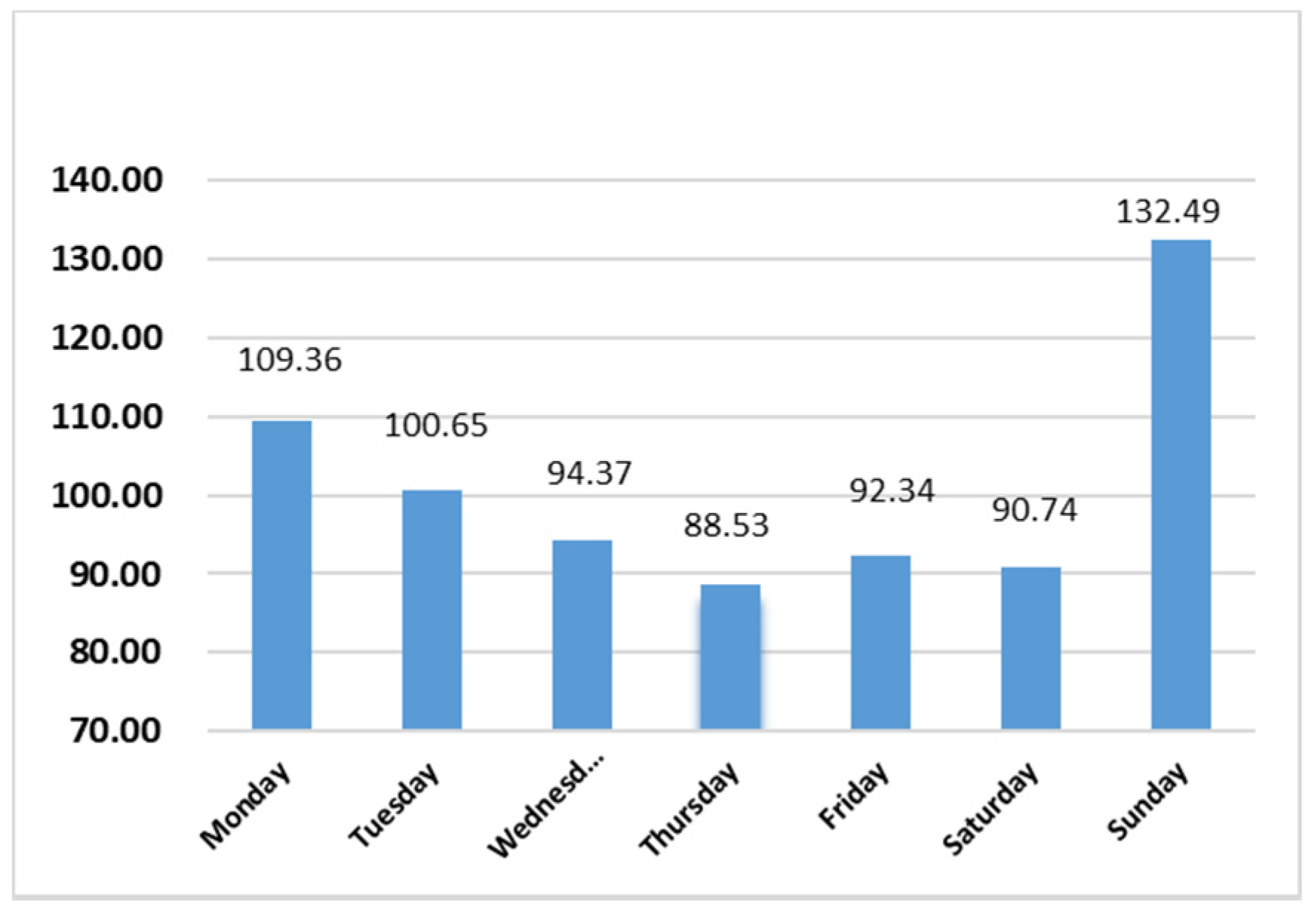
To assess investors’ rational concerns, we utilized the Economic Policy Uncertainty (EPU) Index. As Table 11 illustrates, across weekdays for 1985–2020, the average levels of uncertainty are: (the information has been available on a daily basis since January 1985) 109.36 (Monday), 100.65 (Tuesday), 94.37 (Wednesday), 88.53 (Thursday), 92.34 (Friday), 90.74 (Saturday), and 132.49 (Sunday). The picture that emerges indicates that the EPU on Sundays and Mondays is higher than on the rest of the weekdays. The difference between the EPU average on Mondays and Fridays is 17.02 (t-stat. = 7.92). The difference between Sundays and Fridays is 40.15 (t-stat. = 18.16).
Overall, uncertainty, as reflected in the media and press, is greater on Sundays and Mondays. Our findings are in line with many works arguing that the information content of the news has a sizable effect on the price movements of equity markets (e.g., [38]). Generally, pessimistic or negative news drives investors to react, and security prices slide. In addition, studies examining the empirical properties of the VIX observe a strong negative and asymmetric relationship between news sentiment (for the constituents of the S&P 500 Index) and changes in the VIX [69].
5. Conclusions
We studied the daily behaviour of numerous volatility indices designed to track the expected 30-day volatility for five very active individual US stocks, three US domestic indices, and 10-year Treasury notes and found evidence that returns on these volatility indices are far from being a coin toss. Our findings, which were not affected by extreme events or outliers that can skew the results, held true using different subsamples and statistical methods. They indicated that the expected 30-day volatility of these securities and market indices is systematically higher on Mondays, but lower on Fridays. More specifically, the hike in the looking-forward volatility of 10-year bonds, equity indices, and individual stocks is strongly evident in the first, second, and fifth Mondays of the month. On the other hand, the Friday effect primarily occurs on the first three Fridays of the month. Lastly, the direction of the expected 30-day volatility on Mondays is contingent on Fridays.
Using evidence from psychology, social media, decision-making, transportation studies, and investigations into sleep patterns, we documented that the public tends to dislike Mondays, supporting the premise that individuals’ moods vary across weekdays. In parallel, we found that the mass media tend to express a more pessimistic tone on Sundays and Mondays, as reflected in the Economic Uncertainty Index (EPU). In addition, the tendency to announce negative corporate news on Friday after the markets have closed may also contribute to the patterns we detected. For investors interested in buying or selling volatility products, our findings might help in timing the transaction. Future research may be able to provide further evidence of the deterioration in mood on Monday and its consequences for investors’ risk aversion and asset pricing.
Supplementary Materials
The following supporting information can be downloaded at: www.mdpi.com/article/10.3390/math10111850/s1, Table S1. Summary statistics for the Monday returns categorized by week (continuation of Table 5). Table S2. Summary statistics for the Friday returns categorized by week (continuation of Table 6). Table S3. Changes in the VXAZN on Mondays and Fridays by Year (2011–2020). Table S4. Sign direction of Fridays and Mondays in the Sampled Volatility Indices (two equal subsamples). Table S5. Changes in the VIX on Monday contingent on its direction of change on Friday.
Author Contributions
Conceptualization, Y.I.-B. and M.Q.; methodology, Y.I.-B. and M.Q.; software, Y.I.-B. and M.Q.; validation, Y.I.-B. and M.Q.; formal analysis, Y.I.-B. and M.Q.; investigation, Y.I.-B. and M.Q.; resources, M.Q.; data curation, Y.I.-B. and M.Q.; writing—original draft preparation, Y.I.-B. and M.Q.; writing—review and editing, Y.I.-B. and M.Q.; visualization, Y.I.-B. and M.Q.; supervision, M.Q.; project administration, M.Q. All authors have read and agreed to the published version of the manuscript.
Funding
This research received no external funding.
Institutional Review Board Statement
Not applicable.
Informed Consent Statement
Not applicable.
Conflicts of Interest
The authors declare no conflict of interest.
References
- French, K.R. Stock returns and the weekend effect. J. Financ. Econ. 1980, 8, 55–69. [Google Scholar] [CrossRef]
- Birru, J. Day of the week and the cross-section of returns. J. Financ. Econ. 2018, 130, 182–214. [Google Scholar] [CrossRef]
- Blose, L.E.; Gondhalekar, V. Weekend gold returns in bull and bear markets. Account. Financ. 2013, 53, 609–622. [Google Scholar] [CrossRef]
- Gondhalekar, V.; Mehdian, S. The blue-Monday hypothesis: Evidence based on Nasdaq stocks, 1971–2000. Q. J. Bus. Econ. 2003, 42, 73–89. [Google Scholar]
- Zhang, T.W.; Chueh, H.; Hsu, Y.H. Day-of-the-week trading patterns of informed and uninformed traders in Taiwan’s foreign exchange market. Econ. Model. 2015, 47, 271–279. [Google Scholar] [CrossRef]
- Caporale, G.M.; Plastun, A. The day of the week effect in the cryptocurrency market. Financ. Res. Lett. 2019, 31. [Google Scholar] [CrossRef]
- Aharon, D.Y.; Qadan, M. Bitcoin and the day-of-the-week effect. Financ. Res. Lett. 2019, 31, 415–424. [Google Scholar] [CrossRef]
- Johnston, E.T.; Kracaw, W.A.; McConnell, J.J. Day-of-the-Week Effects in Financial Futures: An Analysis of GNMA, T-Bond, T-Note, and T-Bill Contracts. J. Financ. Quant. Anal. 1991, 26, 23–44. [Google Scholar] [CrossRef] [Green Version]
- Jordan, S.D.; Jordan, B.D. Seasonality in daily bond returns. J. Financ. Quant. Anal. 1991, 26, 269–285. [Google Scholar] [CrossRef]
- Gonzalez-Perez, M.T.; Guerrero, D.E. Day-of-the-week effect on the VIX. A parsimonious representation. N. Am. J. Econ. Financ. 2013, 25, 243–260. [Google Scholar] [CrossRef]
- Plastun, A.; Sibande, X.; Gupta, R.; Wohar, M.E. Rise and fall of calendar anomalies over a century. N. Am. J. Econ. Financ. 2019, 49, 181–205. [Google Scholar] [CrossRef] [Green Version]
- Boubaker, S.; Essaddam, N.; Nguyen, D.K.; Saadi, S. On the robustness of week-day effect to error distributional assumption: International evidence. J. Int. Financial Mark. Inst. Money 2017, 47, 114–130. [Google Scholar] [CrossRef]
- Brusa, J.; Liu, P.; Schulman, C. The “reverse” weekend effect: The US market versus international markets. Int. Rev. Financ. Anal. 2003, 12, 267–286. [Google Scholar] [CrossRef]
- Stivers, C.; Sun, L. Returns and option activity over the option-expiration week for S&P 100 stocks. J. Bank. Financ. 2013, 37, 4226–4240. [Google Scholar] [CrossRef]
- Baker, S.R.; Bloom, N.; Davis, S.J. Measuring Economic Policy Uncertainty. Q. J. Econ. 2016, 131, 1593–1636. [Google Scholar] [CrossRef]
- Areni, C.S.; Burger, M. Memories of “bad” days are more biased than memories of “good” days: Past Saturdays vary, but past Mondays are always blue. J. Appl. Soc. Psychol. 2008, 38, 1395–1415. [Google Scholar] [CrossRef]
- Ryan, R.M.; Bernstein, J.H.; Brown, K.W. Weekends, Work, and Well-Being: Psychological Need Satisfactions and Day of the Week Effects on Mood, Vitality, and Physical Symptoms. J. Soc. Clin. Psychol. 2010, 29, 95–122. [Google Scholar] [CrossRef]
- Wright, W.F.; Bower, G.H. Mood effects on subjective probability assessment. Organ. Behav. Hum. Decis. Process. 1992, 52, 276–291. [Google Scholar] [CrossRef]
- Kostopoulos, D.; Meyer, S. Disentangling investor sentiment: Mood and household attitudes towards the economy. J. Econ. Behav. Organ. 2018, 155, 28–78. [Google Scholar] [CrossRef]
- Qadan, M.; Aharon, D.Y.; Cohen, G. Everybody likes shopping, including the US capital market. Phys. A Stat. Mech. Appl. 2020, 551, 124173. [Google Scholar] [CrossRef]
- Aydogan, B. Sentiment dynamics and volatility of international stock markets. Eurasian Bus. Rev. 2017, 7, 407–419. [Google Scholar] [CrossRef]
- Chen, M.P.; Lee, C.C.; Hsu, Y.C. Investor sentiment and country exchange traded funds: Does economic freedom matter? N. Am. J. Econ. Financ. 2017, 42, 285–299. [Google Scholar] [CrossRef]
- Qadan, M.; Aharon, D.Y. How much happiness can we find in the US fear Index? Financ. Res. Lett. 2019, 30, 246–258. [Google Scholar] [CrossRef]
- Keim, D.B.; Stambaugh, R.F. A further investigation of the weekend effect in stock returns. J. Financ. 1984, 39, 819–835. [Google Scholar] [CrossRef]
- Groth, J.C.; Lewellen, W.G.; Schlarbaum, G.G.; Lease, R.C. An Analysis of Brokerage House Securities Recommendations. Financ. Anal. J. 1979, 35, 32–40. [Google Scholar] [CrossRef]
- Dimson, E.; Marsh, P. An analysis of brokers’ and analysts’ unpublished forecasts of UK stock returns. J. Financ. 1984, 39, 1257–1292. [Google Scholar] [CrossRef]
- Ritter, J.R. The buying and selling behavior of individual investors at the turn of the year. J. Financ. 1988, 43, 701–717. [Google Scholar] [CrossRef]
- Lakonishok, J.; Maberly, E. The weekend effect: Trading patterns of individual and institutional investors. J. Financ. 1990, 45, 231–243. [Google Scholar] [CrossRef]
- Abraham, A.; Ikenberry, D.L. The Individual Investor and the Weekend Effect. J. Financ. Quant. Anal. 1994, 29, 263. [Google Scholar] [CrossRef]
- Singal, V.; Tayal, J. Risky short positions and investor sentiment: Evidence from the weekend effect in futures markets. J. Futur. Mark. 2020, 40, 479–500. [Google Scholar] [CrossRef]
- Bariviera, A.F.; Plastino, A.; Judge, G. Spurious Seasonality Detection: A Non-Parametric Test Proposal. Econometrics 2018, 6, 3. [Google Scholar] [CrossRef] [Green Version]
- Patell, J.M.; Wolfson, M.A. Good news, bad news, and the intraday timing of corporate disclosures. Account. Rev. 1982, 57, 509–527. [Google Scholar]
- Penman, S.H. The distribution of earnings news over time and seasonalities in aggregate stock returns. J. Financ. Econ. 1987, 18, 199–228. [Google Scholar] [CrossRef]
- Dellavigna, S.; Pollet, J.M. Investor Inattention and Friday Earnings Announcements. J. Financ. 2009, 64, 709–749. [Google Scholar] [CrossRef] [Green Version]
- Michaely, R.; Rubin, A.; Vedrashko, A. Further evidence on the strategic timing of earnings news: Joint analysis of weekdays and times of day. J. Account. Econ. 2016, 62, 24–45. [Google Scholar] [CrossRef]
- Carretta, A.; Farina, V.; Martelli, D.; Fiordelisi, F.; Schwizer, P. The Impact of Corporate Governance Press News on Stock Market Returns. Eur. Financ. Manag. 2011, 17, 100–119. [Google Scholar] [CrossRef]
- Tetlock, P.C. Giving Content to Investor Sentiment: The Role of Media in the Stock Market. J. Financ. 2007, 62, 1139–1168. [Google Scholar] [CrossRef]
- Tetlock, P.C.; Saar-Tsechansky, M.; Macskassy, S. More Than Words: Quantifying Language to Measure Firms’ Fundamentals. J. Financ. 2008, 63, 1437–1467. [Google Scholar] [CrossRef]
- Batrancea, L. An Econometric Approach Regarding the Impact of Fiscal Pressure on Equilibrium: Evidence from Electricity, Gas and Oil Companies Listed on the New York Stock Exchange. Mathematics 2021, 9, 630. [Google Scholar] [CrossRef]
- Batrancea, L. The Influence of Liquidity and Solvency on Performance within the Healthcare Industry: Evidence from Publicly Listed Companies. Mathematics 2021, 9, 2231. [Google Scholar] [CrossRef]
- Batrancea, L.; Rus, M.I.; Masca, E.S.; Morar, I.D. Fiscal Pressure as a Trigger of Financial Performance for the Energy Industry: An Empirical Investigation across a 16-Year Period. Energies 2021, 14, 3769. [Google Scholar] [CrossRef]
- Saunders, E.M. Stock prices and wall street weather. Am. Econ. Rev. 1993, 83, 1337–1345. [Google Scholar]
- Kamstra, M.J.; Kramer, L.; Levi, M.D. Winter Blues: A SAD Stock Market Cycle. Am. Econ. Rev. 2003, 93, 324–343. [Google Scholar] [CrossRef] [Green Version]
- Rystrom, D.S.; Benson, E.D. Investor Psychology and the Day-of-the-Week Effect. Financ. Anal. J. 1989, 45, 75–78. [Google Scholar] [CrossRef]
- Yang, C.-M.; Spielman, A.J. The effect of a delayed weekend sleep pattern on sleep and morning functioning. Psychol. Health 2001, 16, 715–725. [Google Scholar] [CrossRef]
- Wen, H.; Sun, J.; Zhang, X. Study on Traffic Congestion Patterns of Large City in China Taking Beijing as an Example. Procedia Soc. Behav. Sci. 2014, 138, 482–491. [Google Scholar] [CrossRef] [Green Version]
- Yang, J.; Lu, F.; Liu, Y.; Guo, J. How does a driving restriction affect transportation patterns? The medium-run evidence from Beijing. J. Clean. Prod. 2018, 204, 270–281. [Google Scholar] [CrossRef]
- Starcke, K.; Brand, M. Decision making under stress: A selective review. Neurosci. Biobehav. Rev. 2012, 36, 1228–1248. [Google Scholar] [CrossRef]
- Stack, S. Temporal Disappointment, Homicide and Suicide: An Analysis of Nonwhites and Whites. Sociol. Focus 1995, 28, 313–328. [Google Scholar] [CrossRef]
- Jessen, G.; Jensen, B.F.; Steffensen, P. Seasons and meteorological factors in suicidal behaviour. Arch. Suicide Res. 1998, 4, 263–280. [Google Scholar] [CrossRef]
- Golder, S.A.; Macy, M.W. Diurnal and Seasonal Mood Vary with Work, Sleep, and Daylength Across Diverse Cultures. Science 2011, 333, 1878–1881. [Google Scholar] [CrossRef] [PubMed] [Green Version]
- Stone, A.A.; Schneider, S.; Harter, J.K. Day-of-week mood patterns in the United States: On the existence of ‘Blue Monday’,’Thank God it’s Friday’ and weekend effects. J. Posit. Psychol. 2012, 7, 306–314. [Google Scholar] [CrossRef]
- Qadan, M.; Idilbi-Bayaa, Y. The day-of-the-week-effect on the volatility of commodities. Resour. Policy 2020, 71, 101980. [Google Scholar] [CrossRef]
- Abu Bakar, A.; Siganos, A.; Vagenas Nanos, E. Does mood explain the Monday effect? J. Forecast. 2014, 33, 409–418. [Google Scholar] [CrossRef] [Green Version]
- Yang, C.-M.; Spielman, A.J.; D’Ambrosio, P.; Serizaw, S.; Nunes, J.; Birnbaum, J. A Single Dose of Melatonin Prevents the Phase Delay Associated with a Delayed Weekend Sleep Pattern. Sleep 2001, 24, 272–281. [Google Scholar] [CrossRef] [Green Version]
- Taylor, A.; Wright, H.R.; Lack, L.C. Sleeping-in on the weekend delays circadian phase and increases sleepiness the following week. Sleep Biol. Rhythm. 2008, 6, 172–179. [Google Scholar] [CrossRef]
- Newey, W.; West, K. A Simple, Positive Semi-Definite, Heteroskedasticity and Autocorrelation Consistent Covariance Matrix. Econometrica 1987, 55, 703. [Google Scholar] [CrossRef]
- Connolly, R.A. A posterior odds analysis of the weekend effect. J. Econ. 1991, 49, 51–104. [Google Scholar] [CrossRef]
- Chiang, C.-H. Stock returns on option expiration dates: Price impact of liquidity trading. J. Empir. Financ. 2014, 28, 273–290. [Google Scholar] [CrossRef]
- Wang, K.; Li, Y.; Erickson, J. A new look at the Monday effect. J. Financ. 1997, 52, 2171–2186. [Google Scholar] [CrossRef]
- Bampinas, G.; Fountas, S.; Panagiotidis, T. The day-of-the-week effect is weak: Evidence from the European real estate sector. J. Econ. Finance 2016, 40, 549–567. [Google Scholar] [CrossRef] [Green Version]
- Schwert, G.W. Anomalies and market efficiency. Handb. Econ. Financ. 2003, 1, 939–974. [Google Scholar]
- Doyle, J.R.; Chen, C.H. The wandering weekday effect in major stock markets. J. Bank. Financ. 2009, 33, 1388–1399. [Google Scholar] [CrossRef] [Green Version]
- You, W.; Guo, Y.; Peng, C. Twitter’s daily happiness sentiment and the predictability of stock returns. Financ. Res. Lett. 2017, 23, 58–64. [Google Scholar] [CrossRef]
- McFarlane, J.M.; Martin, C.L.; Williams, T.M. Mood Fluctuations: Women Versus Men and Menstrual Versus Other Cycles. Psychol. Women Q. 1988, 12, 201–223. [Google Scholar] [CrossRef]
- Hibbert, A.M.; Daigler, R.T.; Dupoyet, B. A behavioral explanation for the negative asymmetric return–volatility relation. J. Bank. Financ. 2008, 32, 2254–2266. [Google Scholar] [CrossRef]
- Andersen, T.G.; Bollerslev, T.; Diebold, F.X.; Labys, P. Modeling and Forecasting Realized Volatility. Econometrica 2003, 71, 579–625. [Google Scholar] [CrossRef] [Green Version]
- Dickey, D.A.; Fuller, W.A. Distribution of the estimators for autoregressive time series with a unit root. J. Am. Stat. Assoc. 1979, 74, 427–431. [Google Scholar]
- Smales, L.A. Risk-on/Risk-off: Financial market response to investor fear. Financ. Res. Lett. 2016, 17, 125–134. [Google Scholar] [CrossRef] [Green Version]
Figure 1.
Average weekly returns resulting from the suggested trading strategy.

Figure 2.
EPU across weekdays. The figure depicts the average of the Economic Uncertainty Policy (EPU) values across weekdays for 1985–2020. On Sundays and Mondays, the EPU is higher than on the rest of the weekdays. The difference between the EPU average on Mondays and Fridays is 17.02 (t-stat. = 7.92). The results are maintained when utilizing two equal subsamples: 1985–December 2002 and January 2003–February 2020.

Table 1.
Volatility indices—general description.
| Security/Index | Ticker Symbol | Sample Period |
|---|---|---|
| Amazon | VXAZN | 16 August 2011–28 February 2020 |
| Apple | VXAPL | 16 August 2011–28 February 2020 |
| Goldman Sachs | VXGSCLS | 6 October 2011–28 February 2020 |
| VXGOG | 16 August 2011–28 February 2020 | |
| IBM | VXIBM | 16 August 2011–28 February 2020 |
| DOW | VXD | 2 October 2013–28 February 2020 |
| NASDAQ | VXN | 10 October 2000–28 February 2020 |
| Russell 2000 | RVX | 15 August 2011–28 February 2020 |
| 10-Year Treasury notes | TYVIX | 30 May 2013–28 February 2020 |
Notes: The table reports the ticker symbol, source, and sample period for the data. The VXAZN is a VIX-style estimate of the expected 30-day volatility of Amazon stock returns. Similarly, VXAPL, VXGSCLS, VXGOG, VXIBM are the VIX-style estimates of Apple, Goldman Sachs, Google, and IBM stock returns, respectively. The VXD, VXN, and RVX are the VIX-style estimates of the expected 30-day volatility of the Dow Jones, NASDAQ-100, and Russell 2000 equity indices, respectively. Finally, TYVIX estimates the expected 30-day volatility of 10-year Treasury notes.
Table 3.
Sign directions of Fridays and Mondays.
| VXAZN (2011:08–2020:02) | VXAPL (2011:08–2020:02) | |||||
| Friday | Monday | Friday | Monday | |||
| Number of times the Index advanced | 156 | 261 | 198 | 243 | ||
| Number of times the Index declined | 276 | 141 | 233 | 158 | ||
| Number of times the Index was unchanged | 2 | 0 | 3 | 1 | ||
| Total | 434 | 402 | 434 | 402 | ||
| Percentage of times the Index advanced (1) (Sign Test t-stat.) | 35.94% *** (5.66) | 64.93% *** (5.99) | 45.62% * (1.54) | 60.45% *** (4.19) | ||
| Percentage of times the Index declined (2) | 63.59% *** (5.66) | 35.07% *** (5.99) | 53.69% * (1.54) | 39.30%*** (4.19) | ||
| Difference (2)-(1) (Sign Test t-stat.) | 27.65% *** (8.47) | 29.85% *** (8.86) | 8.06% ** (2.38) | 21.14%*** (6.13) | ||
| Mean percentage change (t-stat.) | −2.55 *** (−6.25) | 2.23 *** (5.12) | 0.15 (0.46) | 1.26 *** (3.55) | ||
| Median percentage change | −1.59 | 2.21 | −0.45 | 1.44 | ||
| VXGSCLS (2011:10–2020:02) | VXGOG (2011:08–2020:02) | VXIBM (2011:08–2020:02) | ||||
| Friday | Monday | Friday | Monday | Friday | Monday | |
| Number of times the Index advanced | 154 | 235 | 158 | 272 | 183 | 255 |
| Number of times the Index declined | 269 | 160 | 275 | 129 | 241 | 143 |
| Number of times the Index was unchanged | 4 | 1 | 1 | 1 | 10 | 4 |
| Total | 427 | 396 | 434 | 402 | 434 | 402 |
| Percentage of times the Index advanced (1) (Sign Test t-stat.) | 36.07% *** (5.37) | 59.34% *** (3.72) | 36.41% *** (5.57) | 67.66% *** (7.08) | 42.17% *** (2.30) | 63.43% *** (5.39) |
| Percentage of times the Index declined (2) | 63.00% *** (5.37) | 40.40% *** (3.72) | 63.36% *** (5.57) | 32.09% *** (7.08) | 55.53% *** (2.30) | 35.57% *** (5.39) |
| Difference (2)-(1) (Sign Test t-stat.) | 26.93% *** (8.16) | 18.94% *** (5.42) | 26.96% *** (8.24) | 35.57% *** (10.78) | 13.36% *** (3.97) | 27.86% *** (8.22) |
| Mean percentage change (t-stat.) | −0.89 *** (−2.95) | 1.24 *** (3.84) | −2.17 *** (−5.15) | 2.63 *** (6.33) | −0.82 ** (−2.37) | 1.60 *** (4.98) |
| Median percentage change | −1.28 | 1.05 | −1.20 | 2.43 | −0.57 | 1.42 |
| VXD (2013:10–2020:02) | VXN (2000:10–2020:02) | RVX (2011:08–2020:02) | ||||
| Friday | Monday | Friday | Monday | Friday | Monday | |
| Number of times the Index advanced | 126 | 174 | 363 | 536 | 170 | 242 |
| Number of times the Index declined | 196 | 128 | 600 | 366 | 260 | 159 |
| Number of times the Index was unchanged | 1 | 0 | 6 | 5 | 4 | 2 |
| Total | 323 | 302 | 969 | 907 | 434 | 403 |
| Percentage of times the Index advanced (1) (Sign Test t-stat.) | 39.01% *** (3.84) | 57.62% *** (2.65) | 37.46% *** (7.42) | 59.10% *** (5.48) | 39.17% *** (4.13) | 60.05% *** (4.04) |
| Percentage of times the Index declined (2) | 60.68% *** (3.84) | 42.38% *** (2.65) | 61.92% *** (7.42) | 40.35% *** (2.65) | 59.91% *** (4.13) | 39.45% *** (4.04) |
| Difference (2)-(1) (Sign Test t-stat.) | 21.67% *** (3.04) | 15.23% *** (2.25) | 24.46% *** (11.09) | 18.74% *** (8.12) | 20.74% *** (6.24) | 20.60% *** (5.98) |
| Mean percentage change (t-stat.) | −0.53 (−1.25) | 1.60 *** (3.52) | −0.57 *** (−2.92) | 1.68 *** (7.50) | −0.85 *** (−2.91) | 1.94 *** (5.06) |
| Median percentage change | −1.51 | 1.13 | −1.30 | 1.34 | −1.25 | 1.32 |
| TYVIX (2013:05–2020:02) | ||||||
| Friday | Monday | |||||
| Number of times the Index advanced | 119 | 224 | ||||
| Number of times the Index declined | 219 | 88 | ||||
| Number of times the Index was unchanged | 4 | 7 | ||||
| Total | 342 | 319 | ||||
| Percentage of times the Index advanced (1) (Sign Test t-stat.) | 34.80% *** (5.19) | 70.22% *** (7.22) | ||||
| Percentage of times the Index declined (2) | 64.04% *** (5.19) | 27.59% *** (7.22) | ||||
| Difference (2)-(1) (Sign Test t-stat.) | 29.24% *** (7.99) | 42.63% *** (11.89) | ||||
| Mean percentage change (t-stat.) | −1.29 *** (−4.40) | 2.04 *** (7.90) | ||||
| Median percentage change | −1.65 | 1.86 | ||||
Notes: The table illustrates the behaviour of the VIX-style estimator indices on Fridays and Mondays. The results support the premise that Fridays are associated with a decrease in the VIX (meaning an uptick in mood), and Mondays are associated with an increase in the VIX (meaning a deterioration in mood). “***”, “**”, and “*” indicate the statistical significance at the 1%, 5%, and 10% levels, respectively.
Table 4.
Sign directions of Fridays and Mondays after excluding the week on which options expire.
| VXAZN (2011:08–2020:02) | VXAPL (2011:08–2020:02) | VXIBM (2011:08–2020:02) | ||||
| Friday | Monday | Friday | Monday | Friday | Monday | |
| Number of times the Index advanced | 118 | 208 | 149 | 207 | 143 | 213 |
| Number of times the Index declined | 213 | 102 | 181 | 102 | 181 | 94 |
| Number of times the Index was unchanged | 2 | 0 | 3 | 1 | 9 | 3 |
| Total | 333 | 310 | 333 | 310 | 333 | 310 |
| Percentage of times the Index advanced (1) (Sign Test t-stat.) | 35.44% *** (5.09) | 67.10% *** (6.20) | 44.74% * (1.59) | 66.77% *** (5.91) | 42.94% * (1.59) | 68.71% *** (6.59) |
| Percentage of times the Index declined (2) | 63.96% | 32.90% | 54.35% | 32.90% | 54.35% | 30.32% |
| Difference (2)–(1) (Sign Test t-stat.) | 28.53% *** (7.67) | 34.19% *** (9.05) | 9.61% ** (2.49) | 33.87% *** (8.95) | 11.41% *** (2.96) | 38.39% *** (10.34) |
| Mean percentage change (t-stat.) | −3.17 *** (−6.11) | 2.10 (4.11) | −0.11 (−0.31) | 1.74 *** (4.29) | −0.06 (−0.19) | 2.19 *** (6.11) |
| Median percentage change | −1.62 | 2.82 | −0.59 | 2.22 | −0.45 | 2.18 |
| VXGSCLS (2011:10–2020:02) | VXGOG (2011:08–2020:02) | TYVIX (2013:05–2020:02) | ||||
| Friday | Monday | Friday | Monday | Friday | Monday | |
| Number of times the Index advanced | 149 | 207 | 123 | 216 | 92 | 174 |
| Number of times the Index declined | 181 | 102 | 209 | 93 | 169 | 67 |
| Number of times the Index was unchanged | 3 | 1 | 1 | 1 | 2 | 5 |
| Total | 333 | 310 | 333 | 310 | 263 | 246 |
| Percentage of times the Index advanced (1) (Sign Test t-stat.) | 44.74% * (1.59) | 66.77% *** (5.91) | 36.94% *** (4.66) | 69.68% *** (6.93) | 34.98% *** (4.63) | 70.73% *** (6.50) |
| Percentage of times the Index declined (2) | 54.35% | 32.90% | 62.76% | 30.00% | 64.26% | 27.24% |
| Difference (2)–(1) (Sign Test t-stat.) | 9.61% ** (2.49) | 33.87% *** (9.06) | 25.83% *** (6.89) | 39.68% *** (10.75) | 29.28% *** (7.01) | 43.50% *** (10.70) |
| Mean percentage change (t-stat.) | −0.11 (−0.31) | 1.74 *** (4.29) | −1.75 *** (−3.95) | 2.39 *** (5.62) | −1.38 *** (−4.16) | 2.15 *** (7.35) |
| Median percentage change | −0.59 | 2.22 | −0.94 | 2.61 | −1.61 | 1.88 |
| VXD (2013:10–2020:02) | VXN (2000:10–2020:02) | RVX (2011:08–2020:02) | ||||
| Friday | Monday | Friday | Monday | Friday | Monday | |
| Number of times the Index advanced | 100 | 133 | 287 | 433 | 136 | 186 |
| Number of times the Index declined | 148 | 100 | 452 | 264 | 194 | 124 |
| Number of times the Index was unchanged | 1 | 0 | 4 | 4 | 3 | 1 |
| Total | 249 | 233 | 743 | 701 | 333 | 311 |
| Percentage of times the Index advanced (1) (Sign Test t-stat.) | 40.16% *** (2.98) | 57.08% ** (2.16) | 38.63% *** (5.91) | 61.77% *** (6.23) | 40.84% *** (3.01) | 59.81% *** (3.46) |
| Percentage of times the Index declined (2) | 59.44% | 42.92% | 60.83% | 37.66% | 58.26% | 39.87% |
| Difference (2)–(1) (Sign Test t-stat.) | 19.28% *** (2.68) | 14.16% *** (2.05) | 22.21% *** (8.77) | 24.11% *** (9.29) | 17.42% *** (4.56) | 19.94% *** (5.07) |
| Mean percentage change (t-stat.) | −0.38 (−0.79) | 1.78 *** (3.46) | −0.40 * (−1.79) | 2.02 *** (8.03) | −0.53 (−1.57) | 1.94 *** (4.33) |
| Median percentage change | −1.50 | 1.14 | −1.09 | 1.63 | −1.15 | 1.03 |
“***”, “**”, and “*” indicate the statistical significance at the 1%, 5%, and 10% levels, respectively.
Table 5.
Summary statistics for the Monday return categorized by week.
| Panel A: Amazon. | |||||||||
|---|---|---|---|---|---|---|---|---|---|
| First Monday | Second Monday | Third Monday | Fourth Monday | Fifth Monday | First Three Mondays | Last Two Mondays | Difference in the Two Periods | All Mondays | |
| 1.08/2011–02/2020 | |||||||||
| Mean | 3.520 a | 3.208 a | −0.939 | 2.713 a | 3.626 a | 1.529 b | 3.144 a | 1.614 c | 2.228 a |
| T-Statistic | (3.52) | (5.71) | (−0.72) | (3.26) | (4.68) | (2.43) | (5.50) | (1.84) | (5.12) |
| Welch F-test | (3.61) | ||||||||
| Percentage positive | 75.00% | 78.35% | 53.68% | 57.61% | 65.85% | 67.54% | 61.49% | 64.93% | |
| #Obs | 36 | 97 | 95 | 92 | 82 | 228 | 174 | 402 | |
| 2.08/2011−12/2015 | |||||||||
| Mean | 4.343 a | 2.353 a | 0.826 | 2.206 c | 4.098 a | 2.039 a | 3.089 a | 1.05 | 2.493 a |
| T-Statistic | (5.37) | (4.61) | (0.82) | (1.96) | (4.19) | (4.09) | (4.09) | (1.20) | (5.76) |
| Welch F-test | (1.34) | ||||||||
| Percentage positive | 84.21% | 76.00% | 55.10% | 56.25% | 76.19% | 68.64% | 65.56% | 67.31% | |
| #Obs | 19 | 50 | 49 | 48 | 42 | 118 | 90 | 208 | |
| 3.01/2016–02/2020 | |||||||||
| Mean | 2.6 | 4.117 a | −2.819 | 3.267 b | 3.131 b | 0.982 | 3.202 a | 2.22 | 1.943 b |
| T-Statistic | (1.35) | (4.06) | (−1.15) | (2.62) | (2.57) | (0.83) | (3.69) | (1.43) | (2.51) |
| Welch F-test | (2.28) | ||||||||
| Percentage positive | 64.71% | 80.85% | 52.17% | 59.09% | 55.00% | 66.36% | 57.14% | 62.37% | |
| #Obs | 17 | 47 | 46 | 44 | 40 | 110 | 84 | 194 | |
Notes: The table reports the average daily return of the volatility index on each Monday of the month. Monday may appear five times in a certain month. If the first trading day of the month occurs on Monday, we will have five Mondays in that month. If the first trading day of the month is other than Monday, then no Monday is attributed to the first week of the month. The “first three weeks” column reports the average of returns on the first three Mondays combined. The “last two weeks” column reports the average returns of the fourth and fifth Mondays combined. “a”, “b”, and “c” indicate the statistical significance at the 1%, 5%, and 10% levels, respectively. Tests on the other measures are reported in Table S1 in Supplementary Materials.
Table 7.
Changes in the VIX on Monday contingent on its direction of change on Friday.
| Performance of the Index on Monday | VXAZN | VXAPL | |||||
| After an Advance on Friday | After a Decline on Friday | After an Advance on Friday | After a Decline on Friday | ||||
| Number of times the Index advanced | 97 | 152 | 103 | 126 | |||
| Number of times the Index declined | 47 | 94 | 79 | 79 | |||
| Number of times the Index was unchanged | 0 | 0 | 1 | 0 | |||
| Total | 144 | 246 | 183 | 205 | |||
| Percentage of times the Index advanced (t-stat.) | 67.36% *** (4.17) | 61.79% *** (3.69) | 56.28% ** (1.70) | 61.46% *** (3.28) | |||
| Percentage of times the Index declined (t-stat.) | 32.64% *** (4.17) | 38.21% *** (3.69) | 43.17% ** (1.70) | 38.54% *** (3.28) | |||
| Difference (2)–(1) (t-stat.) | 34.72% *** (5.98) | 23.58% *** (5.07) | 13.11% ** (2.43) | 22.93% *** (4.49) | |||
| Mean percentage change (t-stat.) | 3.00 *** (3.85) | 1.39 *** (2.59) | 1.02 * (1.74) | 1.06 ** (2.23) | |||
| Median percentage change | 2.66 | 1.91 | 1.33 | 1.31 | |||
| Performance of the Index on Monday | VXGSCLS | VXGOG | VXIBM | ||||
| After an Advance on Friday | After a Decline on Friday | After an Advance on Friday | After a Decline on Friday | After an Advance on Friday | After a Decline on Friday | ||
| Number of times the Index advanced | 72 | 149 | 90 | 170 | 99 | 143 | |
| Number of times the Index declined | 69 | 90 | 51 | 78 | 64 | 75 | |
| Number of times the Index was unchanged | 1 | 0 | 0 | 1 | 1 | 0 | |
| Total | 142 | 239 | 141 | 249 | 164 | 218 | |
| Percentage of times the Index advanced (t-stat.) | 50.70% (0.17) | 62.34% *** (3.82) | 63.83% *** (3.28) | 68.27% *** (5.77) | 60.37% *** (2.66) | 65.60% *** (4.61) | |
| Percentage of times the Index declined (t-stat.) | 48.59% | 37.66% | 36.17% *** (3.28) | 31.33% *** (5.77) | 39.02% *** (2.66) | 34.40% *** (4.61) | |
| Difference (2)–(1) (t-stat.) | 2.11% (0.34) | 24.69% *** (5.24) | 27.66% *** (4.54) | 36.95% *** (8.37) | 21.34% *** (3.74) | 31.19% *** (6.48) | |
| Mean percentage change (t-stat.) | 0.47 (0.67) | 1.40 *** (3.87) | 2.39 *** (3.58) | 2.64 *** (4.81) | 1.52 *** (2.77) | 1.49 *** (3.67) | |
| Median percentage change | 0.33 | 1.27 | 2.66 | 2.29 | 1.22 | 1.56 | |
| Performance of the Index on Monday | VXD | VXN | RVX | ||||
| After an Advance on Friday | After a Decline on Friday | After an Advance on Friday | After a Decline on Friday | After an Advance on Friday | After a Decline on Friday | ||
| Number of times the Index advanced | 56 | 108 | 186 | 323 | 85 | 147 | |
| Number of times the Index declined | 58 | 67 | 144 | 212 | 70 | 84 | |
| Number of times the Index was unchanged | 0 | 0 | 1 | 4 | 1 | 0 | |
| Total | 114 | 175 | 331 | 539 | 156 | 231 | |
| Percentage of times the Index advanced (t-stat.) | 49.12% (0.43) | 61.71% *** (3.10) | 56.19% ** (2.25) | 59.93% *** (4.61) | 54.49% (1.12) | 63.64% *** (4.15) | |
| Percentage of times the Index declined | 50.88% (0.38) | 38.29% *** (3.00) | 43.50% | 39.33% | 44.87% | 36.36% | |
| Difference (2)–(1) (t-stat.) | 1.75% (0.47) | 23.43% *** (2.66) | 12.69% *** (3.15) | 20.59% *** (6.56) | 9.62% (1.63) | 27.27% *** (5.74) | |
| Mean percentage change (t-stat.) | 1.39 (1.56) | 1.47 *** (2.94) | 1.94 *** (4.32) | 1.30 *** (5.24) | 2.17 *** (2.74) | 1.52 *** (3.80) | |
| Median percentage change | −0.09 | 1.26 | 0.96 | 1.17 | 0.46 | 1.60 | |
| Performance of the Index on Monday | TYVIX | ||||||
| After an Advance on Friday | After a Decline on Friday | ||||||
| Number of times the Index advanced | 68 | 146 | |||||
| Number of times the Index declined | 38 | 47 | |||||
| Number of times the Index was unchanged | 2 | 4 | |||||
| Total | 108 | 197 | |||||
| Percentage of times the Index advanced (t-stat.) | 62.96% *** (2.69) | 74.11% *** (6.77) | |||||
| Percentage of times the Index declined | 35.19% | 23.86% | |||||
| Difference (2)–(1) (t-stat.) | 27.78% *** (4.04) | 50.25% *** (10.92) | |||||
| Mean percentage change (t-stat.) | 1.67 *** (3.27) | 2.27 *** (7.48) | |||||
| Median percentage change | 1.48 | 1.97 | |||||
Notes: A description of the changes in the VIX indices on Monday contingent on its direction of change on Friday. ***, **, and * indicate statistical significance at the 1%, 5%, and 10% levels, respectively. The values in parentheses are the T-Statistics.
Table 8.
A Comparison of changes in the VIX on Monday and on other days of the week contingent on the direction of change the previous day.
Table 8.
A Comparison of changes in the VIX on Monday and on other days of the week contingent on the direction of change the previous day.
| Percentage of Times the Index Advanced | VXAZN | VXAPL | ||||
| On Monday | On Other Days | On Monday | On Other Days | |||
| After an Advance the previous day (t-stat.) | 67.36% *** (4.17) | 47.52% (1.14) | 56.28% ** (1.70) | 47.61% (1.19) | ||
| After a decline the previous day (t-stat.) | 61.79% *** (3.69) | 48.66% (0.39) | 61.46% *** (3.28) | 54.33% *** (2.57) | ||
| Mean Percentage Change | ||||||
| After an Advance the previous day (t-stat.) | 3.00 *** (3.85) | −0.38 * (−1.82) | 1.02 * (1.74) | −0.35 (−1.43) | ||
| After a decline the previous day (t-stat.) | 1.39 *** (2.59) | 0.10 (0.41) | 1.06 ** (2.23) | −0.16 (−0.72) | ||
| Percentage of Times the Index Advanced | VXGSCLS | VXGOG | VXIBM | |||
| On Monday | On Other Days | On Monday | On Other Days | On Monday | On Other Days | |
| After an Advance the previous day (t-stat.) | 50.70% (0.17) | 43.82% *** (3.36) | 63.83% *** (3.28) | 48.75% (0.45) | 60.37% *** (2.66) | 48.42% (0.56) |
| After a decline the previous day (t-stat.) | 62.34% *** (3.82) | 56.46% *** (3.82) | 68.27% *** (3.58) | 52.52% (1.40) | 65.60% *** (4.61) | 51.07% (0.60) |
| Mean Percentage Change | ||||||
| After an Advance the previous day (t-stat.) | 0.47 (0.67) | −0.44 ** (−2.09) | 2.39 *** (3.58) | −0.31 (−1.54) | 1.52 *** (2.77) | −0.57 ** (−2.14) |
| After a decline the previous day (t-stat.) | 1.40 *** (3.87) | −0.16 (−0.79) | 2.64 *** (4.81) | −0.18 (−0.67) | 1.49 *** (3.67) | −0.09 (−0.38) |
| Percentage of Times the Index Advanced | VXD | VXN | RVX | |||
| On Monday | On Other Days | On Monday | On Other Days | On Monday | On Other Days | |
| After an Advance the previous day (t-stat.) | 49.12% (0.43) | 45.09% *** (2.47) | 56.19% *** (2.25) | 43.19% *** (5.56) | 54.49% (1.12) | 42.51% *** (3.99) |
| After a decline the previous day (t-stat.) | 61.71% *** (3.10) | 43.63% *** (3.29) | 59.93% *** (4.61) | 42.45% *** (6.27) | 63.64% *** (4.15) | 46.28% ** (1.73) |
| Mean Percentage Change | ||||||
| After an Advance the previous day (t-stat.) | 1.39 (1.56) | −0.16 (−0.57) | 1.94 *** (4.32) | −0.25 * (−1.90) | 2.17 *** (2.74) | −0.48 ** (−2.45) |
| After a decline the previous day (t-stat.) | 1.47 *** (2.94) | 00.19 (0.61) | 1.30 *** (5.24) | −0.11 (0.83) | 1.52 *** (3.80) | 0.01 (0.07) |
| Percentage of Times the Index Advanced | TYVIX | |||||
| On Monday | On Other Days | |||||
| After an Advance the previous day (t-stat.) | 62.96% *** (2.69) | 43.40% ** (2.25) | ||||
| After a decline the previous day (t-stat.) | 74.11% *** (6.77) | 40.18% *** (3.92) | ||||
| Mean Percentage Change | ||||||
| After an Advance the previous day (t-stat.) | 1.67 *** (3.27) | −0.38 ** (−2.03) | ||||
| After a decline the previous day (t-stat.) | 2.27 *** (7.48) | −0.57 *** (−3.21) | ||||
Notes: A comparison of changes in VIX on Monday and on other days of the week contingent on the direction of change the previous day. ***, **, and * indicate statistical significance at the 1%, 5%, and 10% levels, respectively. The values in parentheses are the T-statistics.
Table 9.
Twitter Happiness Index across weekdays (2008–2020).
| Monday | Tuesday | Wednesday | Thursday | Friday | Saturday | Sunday | |
|---|---|---|---|---|---|---|---|
| Mean | 6.011 *** | 6.009 *** | 6.010 *** | 6.015 *** | 6.031 *** | 6.034 *** | 6.024 *** |
| Med. | 6.010 | 6.010 | 6.010 | 6.010 | 6.030 | 6.030 | 6.020 |
| Max. | 6.250 | 6.210 | 6.250 | 6.360 | 6.340 | 6.290 | 6.260 |
| Min. | 5.770 | 5.880 | 5.870 | 5.890 | 5.780 | 5.870 | 5.840 |
| Stdev. | 0.043 | 0.042 | 0.044 | 0.050 | 0.049 | 0.046 | 0.049 |
| Skew. | −0.039 | 0.309 | 0.841 | 1.556 | 0.545 | 0.247 | 0.352 |
| Kurt. | 5.289 | 3.783 | 6.434 | 9.794 | 7.947 | 4.292 | 4.628 |
| #Obs | 598 | 599 | 599 | 599 | 599 | 596 | 598 |
Notes: The table presents the descriptive statistics of the Twitter Happiness Index across the weekdays. Data come from http://hedonometer.org/index.html and are available from 9 September 2008 to the present. “***” indicates statistical significance at the 1% levels. The values in parentheses are the T-statistics.
Table 10.
Testing the residuals of Equation (3).
| MON | TUE | WED | THU | FRI | ||||
|---|---|---|---|---|---|---|---|---|
| VXAZN | 1.93 a | 0.34 | 0.21 | 0.45 | −2.81 a | 26.26 a | 9.85 a | 22.23 a |
| (5.58) | (1.03) | (0.63) | (1.36) | (−8.40) | ||||
| VXAPL | −1.39 a | −0.24 | −1.27 a | 0.17 | 0.07 | 8.27 a | 2.81 a | 4.11 a |
| (4.10) | (−0.75) | (−3.92) | (0.52) | (0.21) | ||||
| VXGSCLS | 1.29 a | −0.12 | −0.04 | −0.06 | −0.988 a | 7.36 a | 5.38 a | 2.44 c |
| (4.24) | (−0.41) | (−0.13) | (−0.20) | (−3.35) | ||||
| VXGOG | 2.36 a | 0.12 | −0.02 | 0.26 | −2.57 a | 26.48 a | 10.22 a | 16.29 a |
| (6.81) | (0.36) | (−0.05) | (0.79) | (−7.67) | ||||
| VXIBM | 1.55 a | 0.27 | −0.81 b | 0.01 | −0.90 a | 7.97 a | 4.94 a | 2.90 b |
| (4.34) | (0.78) | (−2.37) | (0.03) | (−2.61) | ||||
| VXD | −0.14 | 0.73 c | 0.77 b | −1.05 a | −0.34 | 3.86 a | 0.37 | 5.09 a |
| (−0,34) | (1.87) | (1.98) | (−2.67) | (−0.88) | ||||
| VXN | 1.50 a | −0.13 | −0.36 c | −0.14 | −0.77 a | 19.39 a | 8.21 a | 2.47 c |
| (7.55) | (−0.67) | (−1.89) | (−0.71) | (−4.01) | ||||
| RVX | 1.75 a | 0.08 | −0.23 | −0.38 | −1.11 a | 12.55 a | 6.79 a | 3.00 b |
| (5.78) | (0.29) | (−0.77) | (−1.30) | (−3.79) | ||||
| TYVIX | 2.03 a (7.83) | 0.47 c (1.89) | −0.69 a (−2.77) | −0.20 (−0.80) | −1.49 a (−5.91) | 27.03 a | 9.73 a | 10.86 a |
Notes: The residuals resulting from Equation (3) were regressed against dummies for the weekdays.. The overall picture that emerges indicates that residuals are higher on Mondays and lower on Fridays. Residuals are assumed to reflect the irrational part in the pricing of the volatility index. “a,” “b”, and “c” denote statistical significance at the 1%, 5%, and 10% levels, respectively. The hypothesis about joint equality for the coefficients is rejected. The hypothesis about equality in the coefficients of Monday and Friday is also rejected. Finally, the hypothesis about equality in the coefficients of Tuesday, Wednesday, Thursday, and Friday is also rejected. By Equation (3), . The T-Statistics were Newey–West (HAC, 1987) corrected in all estimations.
Table 11.
Economic Uncertainty Policy across weekdays (Level).
| Panel A. Full Sample. | |||||||
|---|---|---|---|---|---|---|---|
| Monday | Tuesday | Wednesday | Thursday | Friday | Saturday | Sunday | |
| Mean | 109.36 *** | 100.65 *** | 94.37 *** | 88.53 *** | 92.34 *** | 90.74 *** | 132.49 *** |
| Med. | 92.74 | 83.69 | 76.74 | 71.27 | 75.88 | 74.25 | 118.11 |
| Max. | 623.45 | 719.07 | 690.81 | 515.61 | 560.12 | 586.55 | 496.43 |
| Min. | 5.80 | 5.93 | 3.38 | 4.75 | 3.32 | 4.15 | 4.05 |
| Stdev. | 67.65 | 69.96 | 67.18 | 62.39 | 62.16 | 64.78 | 69.97 |
| Skew. | 1.81 | 2.32 | 2.22 | 1.96 | 1.78 | 2.01 | 1.29 |
| Kurt. | 8.85 | 13.44 | 11.79 | 8.65 | 7.95 | 9.94 | 5.23 |
| #Obs | 1834 | 1835 | 1835 | 1835 | 1835 | 1834 | 1834 |
Notes: The table reports the descriptive statistics of the Economic Policy Uncertainty Index developed by [15]. The overall picture indicates that uncertainty, as reflected in US newspapers, is greater on Sunday and Monday. “***” indicates statistical significance at the 1% levels.
Publisher’s Note: MDPI stays neutral with regard to jurisdictional claims in published maps and institutional affiliations. |
© 2022 by the authors. Licensee MDPI, Basel, Switzerland. This article is an open access article distributed under the terms and conditions of the Creative Commons Attribution (CC BY) license (https://creativecommons.org/licenses/by/4.0/).
Share and Cite
MDPI and ACS Style
Idilbi-Bayaa, Y.; Qadan, M. Tell Me Why I Do Not Like Mondays. Mathematics 2022, 10, 1850. https://doi.org/10.3390/math10111850
AMA Style
Idilbi-Bayaa Y, Qadan M. Tell Me Why I Do Not Like Mondays. Mathematics. 2022; 10(11):1850. https://doi.org/10.3390/math10111850
Chicago/Turabian StyleIdilbi-Bayaa, Yasmeen, and Mahmoud Qadan. 2022. "Tell Me Why I Do Not Like Mondays" Mathematics 10, no. 11: 1850. https://doi.org/10.3390/math10111850
Note that from the first issue of 2016, this journal uses article numbers instead of page numbers. See further details here.