Scalable Cell-Free Massive MIMO with Multiple CPUs

Abstract

In this paper, we consider the uplink of a scalable cell-free massive MIMO (CF-M-MIMO) system where user equipments (UEs) are served only by a subset of access points (APs). All APs are physically divided into predetermined “real clusters”, which are linked to different cooperative central processing units (CPUs). Based on the cooperative nature of the considered communications framework, we assume that each UE is affiliated with a “virtual cluster”, which is associated with some APs coming from different real clusters. Thanks to the degrees of cooperation among multiple CPUs, the uplink spectral efficiencies (SEs) of four different levels are analyzed. To achieve system scalability, the CF-M-MIMO system with multiple CPUs is introduced, which leads to lower SE. To this end, we design a joint combining method based on statistical channel state informations (CSIs), which not only has low complexity but also improves the SE of the system. Simulation results indicate that the average rate of our proposed method can be improved by about 30%.

1. Introduction

The demand of user equipments (UEs) for high transmission rates and wide communication coverage are boosting the evolution of wireless network architecture. The distributed communication system [1] cooperates through multiple access points (APs) to realize coherent combinations, reduce interference and supply macro diversity gain, so as to obtain high spectral efficiency. Distributed antenna systems (DAS), coordinated multipoint with joint transmission (CoMP-JT) and network multiple-input multiple-output (Network MIMO) are suggested as some examples of cellular distributed systems with the joint transmission of multiple APs [2,3,4]. Theoretically, the interference between cells can be mitigated by designing the cooperation of adjacent clusters, in which the APs belonging to different clusters jointly serve all UEs in the region. However, the cooperation requires perfect channel state informations (CSIs) to be exchanged, which is not scalable in practice [5]. In addition, the inter-cell or out-of-cluster interference caused by the cellular mode cannot be suppressed, which also results in performance limitations. In fact, the standardization of CoMP-JT in cellular networks has not been widely promoted.

Recently, massive MIMO has become the key technology of 5G. Massive MIMO has the ability to improve the spectral efficiencie (SE) by about 10 times over small cell networks [6,7], by improving the base station (BS) hardware instead of increasing the number of BSs. The SE gain benefits from a lot of antennas in each BS, which are applied for digital beamforming and, particularly, to spatially multiplex multiple UEs on the same time-frequency resource [8,9]. With the development of massive MIMO technology [10], the interest in distributed massive MIMO systems has been revived. Distributed massive MIMO systems are equipped with many BSs, and each BS has an array formed by a large number of antennas. Similar to CoMP-JT, distributed massive MIMO systems can be designed for joint transmission [7,11] through multiple BSs, and are expected to achieve better performance than cellular systems. Therefore, many different architectures based on massive MIMO have been proposed.

A recent system architecture, referred to as cell-free massive MIMO (CF-M-MIMO), was proposed in [12,13,14,15]. The basic idea is that a large number of APs are distributed in a wide area to serve a small number of UEs. A central processing unit (CPU) connects to these APs, which can also be called an edge-cloud processor [16] or cloud radio access network (C-RAN) data center [17].

1.1. Related Work

Compared with traditional small cell systems, CF-M-MIMO systems have made changes in the way of serving the UE. Unlike small cell systems in that each UE is served by only one AP, CF-M-MIMO systems allow the CPU to connect multiple APs for digital beamforming [11], which provides coordinated transmission for several UEs on the same time-frequency resource. Early studies have shown that appropriate signal processing methods, such as regularized zero-forcing (RZF) or minimum mean-squared error (MMSE) precoding in the downlink, can be used separately at each CPU to suppress the interference from other APs connected to the same CPU [18,19,20], rather than cooperate with other CPUs.

CF-M-MIMO combines the benefits of using time division duplex (TDD) mode [10], distributed massive MIMO technology and user-centric transmission. The TDD operation relies on channel reciprocity to obtain CSIs [21], which can reduce the fronthaul burden. Thanks to the antennas with uniform amplitude distribution that can more effectively combat shadow fading, the distributed massive MIMO systems can have greater coverage than collocated massive MIMO systems [22]. In addition, the user-centric approach enables CF-M-MIMO systems to mitigate the inter-cell interference [23]. Without cell boundaries, all the UEs are considered to be surrounded by a large number of APs, thus the boundary effect can be eliminated [13,23]. Although recent works have shown that CF-M-MIMO systems have significant advantages in many aspects, there is still a big gap between theoretical analysis and practical application. For example, the key assumption that all the APs are controlled by a single CPU is hard to achieve scalability in CF-M-MIMO.

Actually, the implementation of the scalable CF-M-MIMO mainly faces two problems.

• Despite [18] having proved that excellent performance can be achieved when all the APs are connected to a single CPU for joint transmission, it is difficult to let a single CPU control all the APs when the number of APs is large. Moreover, joint transmission requires a single CPU to centralize the signal processing, which puts high demands on the CPU’s processing capacity.
• The traditional precoding and power control of CF-M-MIMO act on the overall APs and UEs, which are difficult to realize in practice. Although a series of studies have proved the superiority of the final results [18,24,25], the complexity of these algorithms grows polynomially with the number of APs or UEs. Moreover, each AP needs to transmit instantaneous CSIs to the CPU, which is also difficult to achieve scalability when there are a large number of APs in the CF-M-MIMO systems.

The scalability of the power control or precoding algorithms has been considered in [26,27,28,29,30]. The article [26] concentrated on the scalability of CF-M-MIMO with a single CPU. If the CPU only controls a partial number of APs serving each UE, the complexity of precoding or power control is not increased with the number of APs. The introduction of the dynamic cooperation clustering (DCC) network makes the above method possible. In papers [28,29], the authors proposed the power allocation strategies based on long-term fading, which avoid a large amount of information exchanging among multiple CPUs and APs. The local partial zero-forcing precoding and combining were considered in [27,30], which depend on the large-scale fading and act on partial UEs and APs. These papers provide feasible methods to achieve scalable implementations. However, these papers mentioned above only focus on the first issue, but do not discuss the second one.

In [31], the author considered the scenario of multiple CPUs and discussed the scalability aspects of CF-M-MIMO. However, cooperation among multiple CPUs is less understood in the literature and still open for investigation. In order to enhance the competitiveness of multiple CPUs systems, how to exchange the information for cooperation among multiple CPUs is an essential problem. As the above considerations demonstrate, exchanging instantaneous CSIs for joint transmission achieves high performance gain [18,32,33]. However, this method puts a great burden on the backhaul, thus it is unscalable. Since the statistical CSIs remain unchanged for a long time, it is considered to be available in a scalable network. In summary, how to use statistical CSIs for cooperative transmission is a key problem. In [34], the authors did not fully exploit the potential performance of CF-M-MIMO with multiple CPUs when statistical CSIs can be exchanged among multiple CPUs. In [34], the estimation of signals from UEs was calculated by simply taking the average of all the signals, which led to a large spectral efficiency (SE) loss. In addition, the authors did not take into account the DCC network, which made it difficult for the network to achieve scalability. All of these motivate the current work to focus on cooperation among multiple CPUs with statistical CSIs. The contributions of this paper are summarized as follows:

• We consider a taxonomy with four different implementations of CF-M-MIMO with multiple CPUs, which are classified by different degrees of cooperation among the CPUs. The four different levels of cooperation can be called centralized connectivity, distributed connectivity and complex processing, distributed connectivity and simple processing, and no connectivity, respectively. The difference of these levels is shown in

  Table 1. Type of CSIs that needs to exchange among CPUs, and the comparison of different levels of cooperation.

  	Type of CSIs	Level of Computational Complexity
  Level 4 centralized connectivity	instantaneous CSIs	high
  Level 3 distributed connectivity and complex processing	statistical CSIs	medium
  Level 2 distributed connectivity and simple processing	statistical CSIs	low
  Level 1 no connectivity	−	lowest

  . We derive novel SE expressions for different levels of multiple CPUs cooperation in the uplink transmission. In addition, unlike most scenarios that specify the number of CPUs participating in the service, we consider a completely user-centric way to select APs.
• We propose a novel signal processing algorithm for cooperation among multiple CPUs. Each CPU processes the local information from its APs, and then transmits these signals to a CPU for final decoding. Based on the generalized Rayleigh quotient, we use simple weighted processing to linearly combine received signals from multiple CPUs with statistical CSIs.
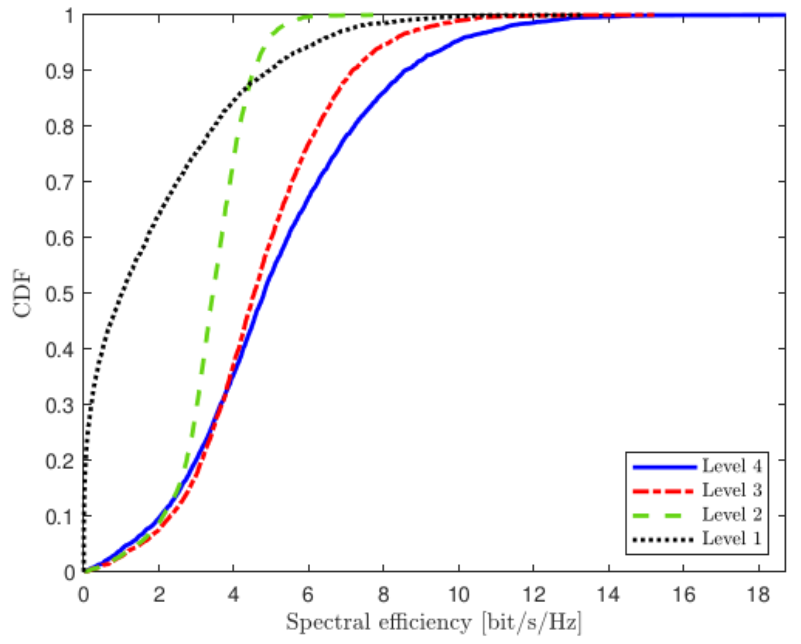
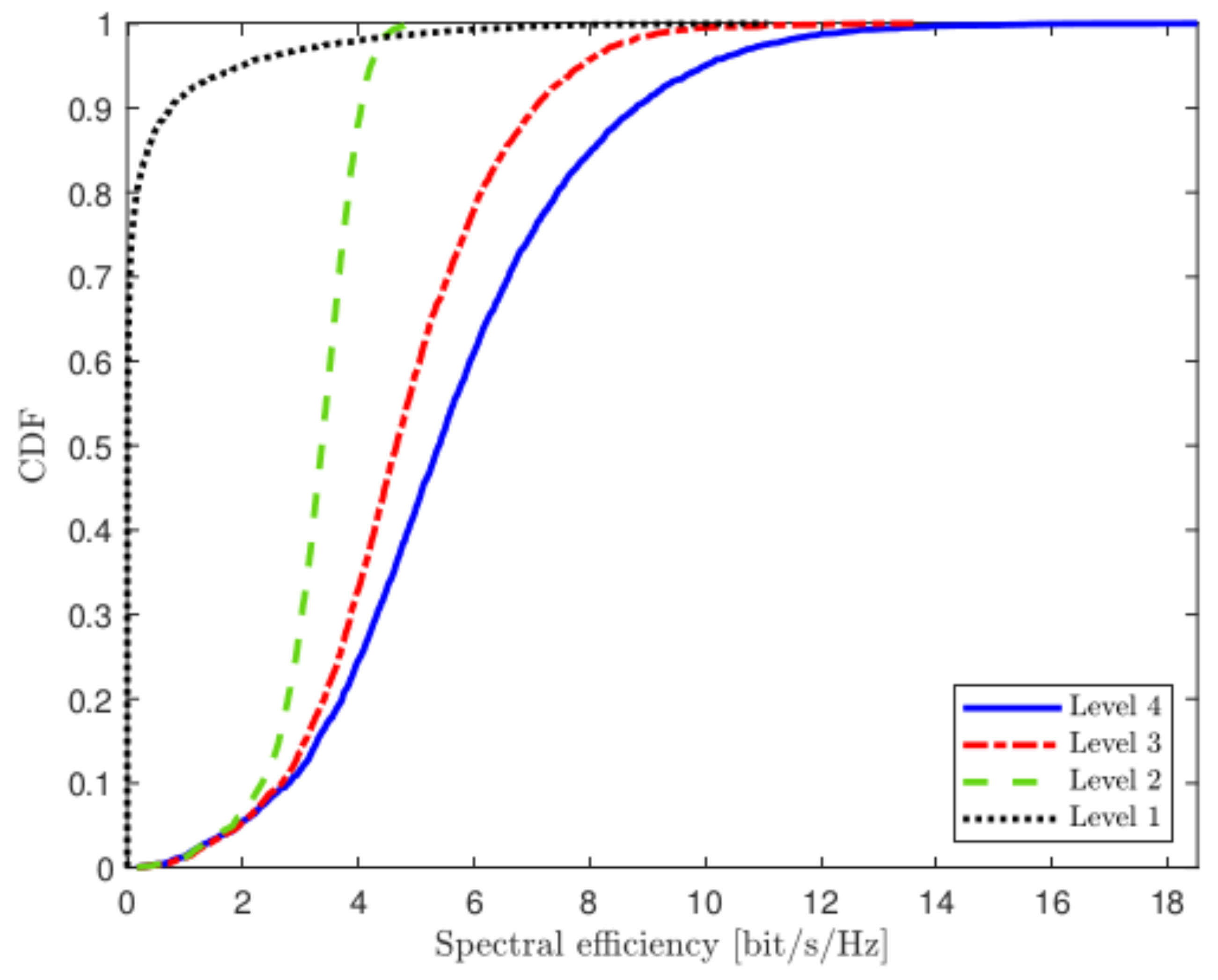
• We compare the performance of different cooperation levels. Monte Carlo simulation results show that our proposed distributed connectivity scheme can achieve scalability with lower backhual burden, and the performance loss is negligible compared to the centralized connectivity scheme.

1.2. Paper Structure

The rest of this paper is organized as follows. Section 2 defines the uplink of CF-M-MIMO system with multiple CPUs. Next, Section 3 presents the four levels of CPU cooperation. Simulation results compare the performance of the four levels of CPUs cooperation in Section 4. Finally, Section 5 concludes this paper.

2. System Model

Notation: Boldface lowercase letters denote column vectors and boldface uppercase letters denote matrices. The superscripts ()${}^{*},{\left(\right)}^{\mathrm{T}}$, and ()${}^{\mathrm{H}}$ indicate transpose, conjugate and transpose. Since we cannot guarantee full rank of matrices, we use ${\left(·\right)}_{}^{†}$ to denote the matrix pseudoinverse. The $n\times n$ identity matrix stands for ${\mathrm{I}}_{\mathrm{N}}$. The $diag\left({\mathbf{h}}_1,\dots ,{\mathbf{h}}_n\right)$ is used to denote a block-diagonal matrix. $z\sim \mathcal{CN}\left(0,{\sigma }^2\right)$ denotes a circularly symmetric complex Gaussian random variable (RV) z with zero mean and variance ${\sigma }^2$. $\left|\mathcal{Z}\right|$ is applied to denote the cardinality of the set $\mathcal{Z}$.

We consider a CF-M-MIMO system operating in TDD mode, which consists of K single-antenna UEs, L single-antenna APs and U CPUs as shown in Figure 1. All of these APs are divided into U predetermined real clusters (RCs). Each RC is connected to a different CPU via error-free fronthaul links. The indexes of the APs belonging to the u-th RC are included in the subsets ${\mathcal{P}}_u^{}$. All CPUs are interconnected through error-free backhual links and can be cooperated with each other. The generic k-th UE is served by a subset of the APs and the subset is termed virtual cluster (VC). We define by ${\mathcal{Z}}_k^{}$ the sets consisting of AP indexes in the k-th VC. Although the RCs are non-overlapped, due to the connection between different CPUs, the VCs can be overlapped so that CPUs can cooperate to serve UEs in the network. In addition, ${\mathcal{A}}_{ku}$ is used to define the set including the AP indexes belonging to both the u-th RC and the k-th VC, i.e.,

$${\mathcal{A}}_{ku}=\left\{l\in {\mathcal{P}}_u^{}:l\in {\mathcal{Z}}_k^{}\right\}.$$

(1)

If the set ${\mathcal{A}}_{ku}$, is not empty, i.e., at least one AP in ${\mathcal{P}}_u^{}$ serves the k-th UE, then the u-th CPU serves UE k.

The channel between AP l and UE k can be modeled as:

$$h_{kl}={\beta }_{kl}^{1/2}{g}_{kl},$$

(2)

where ${\beta }_{kl}$ is the large-scale fading coefficient related to geometric path loss and shadow fading and $g_{mk}$ is the small scale fading. The large-scale fading coefficient ${\beta }_{kl}$ changes tardily, and thus, can be traced and acquired. We assume that $g_{kl}$, $l=1,\dots ,L,k=1,\dots ,K$, are independent and identically distributed (i.i.d.) $\mathcal{CN}(0,1)$ RVs.

2.1. Channel Estimation

We consider the uplink with ${\tau }_{\mathrm{c}}$ channel use, which consists of ${\tau }_{\mathrm{p}}^{}$ channels for transmitting pilots and ${\tau }_{\mathrm{c}}-{\tau }_{\mathrm{p}}^{}$ channels for payload data. In the pilot transmission phase, ${\tau }_{\mathrm{p}}^{}$ mutually orthogonal ${\tau }_{\mathrm{p}}^{}$-length pilot signals ${\mathit{\phi }}_{\mathbf{1}}$, ${\mathit{\phi }}_{\mathbf{2}}$…${\mathit{\phi }}_{{\mathit{\tau }}_{\mathit{p}}^{}}$ are applied for channel estimation, where ${∥{\mathit{\phi }}_{\mathit{n}}∥}_{}^2={\tau }_{\mathrm{p}}^{}$. The case of practical interest is a big network with ${\tau }_{\mathrm{p}}^{}<K$, which means that more than one UE is assigned to each pilot. This is so-called pilot contamination that degrades the system performance. We suppose that $t_k\in \left\{1,\dots ,{\tau }_p\right\}$ is the index of the pilot assigned to UE k and ${\mathcal{G}}_k^{}\subset \left\{1,2...K\right\}$ denotes the subset of UEs which are assigned the same pilot as UE k. When all UEs send their pilots, the received signal at AP l is:

$${\mathbf{y}}_l^{pilot}=\sum _{i=1}^K\sqrt{p_i}{h}_{il}{\mathit{\phi }}_{t_k}^{\mathrm{H}}+{\mathbf{n}}_l,$$

(3)

where $p_i$ is the transmission power of UE i, ${\mathbf{n}}_l\in {\mathbb{C}}^{{\tau }_{\mathrm{p}}^{}\times 1}$ is the noise vector whose elements are i.i.d. $\mathcal{C}\mathcal{N}(0,{\sigma }_{}^2)$ RVs. According to the received signal ${\mathbf{y}}_l^{pilot}$, AP l places it on the project with ${\mathit{\phi }}_{t_k}^{*}$ to obtain ${\widehat{y}}_l$, which is given by:

$$\begin{array}{cc}\hfill {\widehat{y}}_l& =\sum _{i=1}^K\frac{\sqrt{p_i}}{\sqrt{{\tau }_p}}{h}_{il}{\mathit{\phi }}_{t_k}^{\mathrm{H}}{\mathit{\phi }}_{t_k}^{*}+\frac{1}{\sqrt{{\tau }_p}}{\mathbf{n}}_l{\mathit{\phi }}_{t_k}^{*}\hfill \\ \hfill & =\sum _{i\in {\mathcal{G}}_k}\sqrt{p_i{\tau }_p}{h}_{il}+\frac{1}{\sqrt{{\tau }_p}}{\mathbf{n}}_l{\mathit{\phi }}_{t_k}^{*}.\hfill \end{array}$$

(4)

Applying standard formulas from paper [13], the minimum mean-squared error (MMSE) estimate of $h_{kl}$ is expressed as:

$${\widehat{h}}_{kl}=\sqrt{p_k{\tau }_p}{\beta }_{kl}{\Psi }_{t_{k}l}^{-1}{\widehat{y}}_l^{},$$

(5)

where:

$${\Psi }_{t_{k}l}=\mathbb{E}\left\{{\widehat{y}}_l^{}{\widehat{y}}_l^{\mathrm{H}}\right\}=\sum _{i\in {\mathcal{G}}_k^{}}{\tau }_p{p}_i{\beta }_{il}+{\sigma }_{}^2.$$

(6)

We define the estimation error as ${\tilde{h}}_{kl}=h_{kl}-{\widehat{h}}_{kl}$, where ${\widehat{h}}_{kl}\sim \mathcal{CN}\left(0,p_k{\tau }_p{\beta }_{kl}{\Psi }_{t_{k}l}^{-1}{\beta }_{kl}\right)$ and ${\tilde{h}}_{kl}\sim \mathcal{CN}\left(0,C_{kl}\right)$ with:

$$C_{kl}={\beta }_{kl}-p_k{\tau }_p{\beta }_{kl}{\Psi }_{t_{k}l}^{-1}{\beta }_{kl}.$$

(7)

The channel estimation error mainly caused by pilot contamination.

2.2. Uplink Payload Transmission

During the uplink transmission, all the UEs transmit signals to the APs. In the AP cluster ${\mathcal{A}}_{ku}$, the signal received by AP l is:

$$y_l^{\mathit{ul}}=\sum _{i=1}^K{h}_{il}{s}_i+n_{u,l},$$

(8)

where $s_i$ is information-bearing signal sent by UE i with $\mathbb{E}\left({\left|s_i\right|}^2\right)=1$ and $n_{u,l}\sim \mathcal{CN}\left(0,1\right)$ is additive noise at AP l.

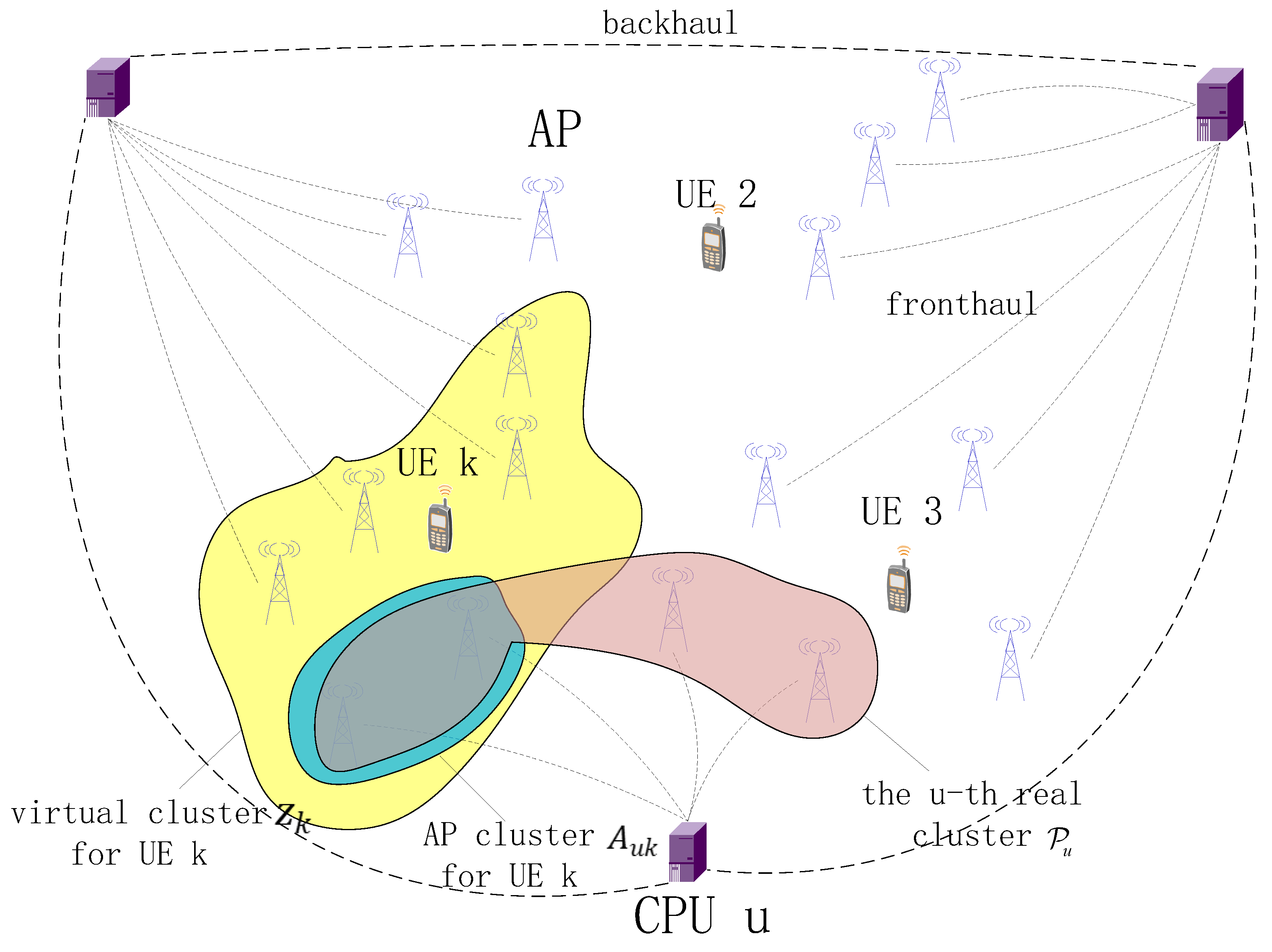
2.3. Dynamic Cooperation Clustering Network

The DCC network was considered in [20,26] to achieve scalability in CF-M-MIMO, and we use it to set the VCs. It is obtained by stipulating a number $d_{il}$, for $i=1,\dots ,K$ and $l=1,\dots ,L$, which set the subset of APs that serve UEs. More specifically, $d_{il}$ is 1 if AP l is allowed to convey and decode signals from UE i and 0 otherwise. The DCC network does not alter the received uplink signals since all the APs physically receive the signals from all the UEs. However, only a subset of the APs is participating in signal detection. This is equivalent to setting $d_{il}^{}$ as:

$$d_{il}=\left\{\begin{array}{cc}1\hfill & \mathrm{if}l\in {\mathcal{Z}}_i\\ 0\hfill & \mathrm{if}l\notin {\mathcal{Z}}_i\end{array}\right..$$

(9)

3. Multiple CPUs Cooperative Transmission

In order to obtain better performance, each VC appoints a $Master$ $CPU$ that possesses high computational resources to receive information from other CPUs for joint processing. Four different levels of cooperation are considered below.

3.1. Level 4: Centralized Connectivity

The highest level of multiple CPUs cooperation network is that all the CPUs share their instantaneous CSIs with the Master CPU. Thus, the Master CPU can be capable of designing an overall MMSE combining matrix. In other words, all the CPUs except the Master CPU play as relays without processing signals from the APs and forward all signals to the Master CPU [35]. In fact, it is equivalent to setting a large VC for each UE, where all the APs in the large VC are managed by a single CPU. In the uplink transmission phase, the received signal at the Master CPU is expressed as:

$$\begin{array}{cc}\hfill {\widehat{s}}_k& =\sum _{l=1}^L{v}_{kl}^{\mathrm{H}}{d}_{kl}{y}_l^{ul}\hfill \\ \hfill & ={\mathbf{v}}_k^{\mathrm{H}}{\mathbf{D}}_k{\mathbf{h}}_k{s}_k+\sum _{i=1,i\ne k}^K{\mathbf{v}}_k^{\mathrm{H}}{\mathbf{D}}_k{\mathbf{h}}_i{s}_i+{\mathbf{v}}_k^{\mathrm{H}}{\mathbf{D}}_k\mathbf{n},\hfill \end{array}$$

(10)

where ${\mathbf{D}}_k^{}$ = diag$[d_{k1}^{},\dots ,d_{kL}^{}]\in {\mathbb{C}}^{L\times L}$ is a block diagonal matrix, $\mathbf{n}={\left[n_1,\dots ,n_L\right]}^{\mathrm{H}}\in {\mathbb{C}}^{L\times 1}$ denotes noise vector at the k-th VC and ${\mathbf{h}}_k={\left[h_{k1},\dots ,h_{kL}\right]}^{\mathrm{H}}\in {\mathbb{C}}^{L\times 1}$ is the collective channel vector at the k-th VC.

Although the capacity of Level 4 with perfect CSIs is supposed to be known in some cases [35], the ergodic capacity is usually unknown when taking into account imperfect CSIs. Nevertheless, we can utilize the lower bounds of standard capacity to analyze the performance [36], which can be used to achieve the following SE.

Proposition 1.

At Level 4, an achievable SE for UE k is:

$${\mathrm{SE}}_k^{\left(4\right)}=\left(1-\frac{{\tau }_p}{{\tau }_c}\right)\mathbb{E}\left\{{log}_2\left(1+{\mathrm{SINR}}_k^{\left(4\right)}\right)\right\},$$

(11)

and a lower bound of capacity to signal-to-interference-and-noise ratio (SINR) for UE k is given by:

$${\mathrm{SINR}}_k^{\left(4\right)}=\frac{p_k{\left|{\mathbf{v}}_k^{\mathrm{H}}{\mathbf{D}}_k^{}{\widehat{\mathbf{h}}}_k\right|}^2}{{\displaystyle \sum _{i=1,i\ne k}^K}{p}_i{\left|{\mathbf{v}}_k^{\mathrm{H}}{\mathbf{D}}_k^{}{\widehat{\mathbf{h}}}_i\right|}^2+{\mathbf{v}}_k^{\mathrm{H}}{\mathbf{L}}_k{\mathbf{v}}_k}$$

(12)

with:

$${\mathbf{L}}_k={\mathbf{D}}_k\left(\sum _{i=1}^K{p}_i{\mathbf{C}}_i+{\sigma }_{}^2{\mathbf{I}}_L\right){\mathbf{D}}_k,$$

(13)

where${\mathbf{C}}_i=diag[C_{i1}^{},\dots ,C_{iL}^{}]\in {\mathbb{C}}^{L\times L}$.

Proof. 

This proof follows the same steps as the proof of [18] for CF-M-MIMO with a single CPU.    □

The pre-log factor $1-\frac{{\tau }_p}{{\tau }_c}$ in (11) denotes the fraction of channel uses which are utilized for uplink data transmission. The term ${\mathrm{SINR}}_k^{\left(4\right)}$ uses the form as effective instantaneous SINR [24]. The numerator is the desired signal power received over the estimated channel, and the denominator is interference plus noise. We note that ${\mathrm{SINR}}_k^{\left(4\right)}$ is in the form of the generalized Rayleigh quotient. Hence, the MMSE combining can be achieved to maximize (12).

Corollary 1.

According to the generalized Rayleigh quotient [24], the ${\mathrm{SINR}}_k^{\left(4\right)}$ (12) for UE k is maximized by the MMSE combining:

$${\mathbf{v}}_k=p_k{\left(\sum _{i=1}^K{p}_i{\mathbf{D}}_k^{}{\widehat{\mathbf{h}}}_i{\widehat{\mathbf{h}}}_i^{\mathrm{H}}{\mathbf{D}}_k^{}+{\mathbf{L}}_k\right)}^{†}{\mathbf{D}}_k^{}{\widehat{\mathbf{h}}}_k,$$

(14)

which obtains the maximum value:

$${\mathrm{SINR}}_k^{\left(4\right)}=p_k{\mathbf{D}}_k^{\mathrm{H}}{\widehat{\mathbf{h}}}_k{\left(\sum _{i=1}^K{p}_i{\mathbf{D}}_k^{}{\widehat{\mathbf{h}}}_i{\widehat{\mathbf{h}}}_i^{\mathrm{H}}{\mathbf{D}}_k^{}+{\mathbf{L}}_k\right)}^{†}{\mathbf{D}}_k^{}{\widehat{\mathbf{h}}}_k.$$

(15)

Proof. 

It follows from [24] (Lemma B.10), and note that (12) is a generalized Rayleigh quotient with respect to ${\mathbf{v}}_k$.    □

Table 2. Number of complex scalars that other CPUs send to the Master CPU through the backhaul, either in each coherence block or for each realization of the UE locations/statistics.

	Each Coherence Block	Statistical Parameters
Level 4	${\tau }_{\mathrm{c}}\left|{\mathcal{Z}}_k^{}\right|-{\tau }_{\mathrm{c}}\left|{\mathcal{A}}_{MCk}\right|$	$\left(K\left|{\mathcal{Z}}_k^{}\right|\right)/2$
Level 3	$K({\tau }_{\mathrm{c}}-{\tau }_{\mathrm{p}}^{})\left(\right|{\mathcal{U}}_k^{}|-1)$	$K\left|{\mathcal{Z}}_k^{}\right|+\left(\right|{\mathcal{U}}_k^{}{|}^2{K}^2+K|{\mathcal{U}}_k^{}\left|\right)/2$
Level 2	$K({\tau }_{\mathrm{c}}-{\tau }_{\mathrm{p}}^{})\left(\right|{\mathcal{U}}_k^{}|-1)$	−
Level 1	−	−

shows the number of complex scalars that the other CPUs send to the Master CPU through the backhaul, in which ${\mathcal{A}}_{MCk}\subset {\mathcal{Z}}_k^{}$ includes the indexes of the APs that serve UE k and are controlled by the Master CPU. In each coherence block, all the CPUs except the Master CPU need to send ${\tau }_{\mathrm{c}}\left|{\mathcal{Z}}_k^{}\right|-{\tau }_{\mathrm{c}}\left|{\mathcal{A}}_{MCk}\right|$ complex scalars to the Master CPU. In addition, the collective channel $\left\{{\mathbf{D}}_k{\mathbf{h}}_k:k=1,\dots ,K\right\}$ are supposedly available at the Master CPU, which can be expressed as $\left(K\left|{\mathcal{Z}}_k^{}\right|\right)/2$ complex scalars.

Although centralized processing can obtain the best performance in most cases, it puts high demands on bandwidth and the delay of backhaul. This poses a difficulty in achieving scalability in CF-M-MIMO. In addition, it is difficult for the Master CPU to handle a large amount of instantaneous CSIs. Therefore, a more practical connection mode is considered below.

3.2. Level 3: Distributed Connectivity and Complex Processing

This solution requires that statistical CSIs can be exchanged among multiple CPUs. Instead of setting a large VC and sending all the signals to the Master CPU for unified processing, we select a set of CPUs for each UE to reduce the pressure of backhaul. We assume that the CPU in each RC can deal with its signals collected from APs, and then these signals are transferred to the Master CPU for final decoding.

Based on the neighborhood criterion, we suppose that the corresponding setting of the DCC framework in the u-th RC is ${\mathbf{D}}_{ku}^{}$ = diag$[b_{k1}^{},\dots ,b_{k|{\mathcal{P}}_u^{}|}^{}]\in {\mathbb{C}}^{|{\mathcal{P}}_u^{}|\times |{\mathcal{P}}_u^{}|}$, where $b_{kl}$ can be written as:

$$b_{kl}=\left\{\begin{array}{cc}1\hfill & \mathrm{if}l\in {\mathcal{A}}_{ku}\\ 0\hfill & \mathrm{if}l\notin {\mathcal{A}}_{ku}\end{array}\right..$$

(16)

We assume by ${\mathcal{U}}_k^{}$ the sets consisting of the CPU indexes in the k-th VC. Unlike Level 4, each CPU can utilize the local channel estimation to design the combining. Let ${\mathbf{v}}_{ku}\in {\mathbb{C}}^{|{\mathcal{P}}_u^{}|\times 1}$ be the local combining vector that CPU u determines for UE k. The local estimates at CPU u is:

$${\widehat{s}}_{ku}={\mathbf{v}}_{ku}^{\mathrm{H}}{\mathbf{D}}_{ku}^{}{\mathbf{h}}_{ku}{s}_k+\sum _{i=1,i\ne k}^K{\mathbf{v}}_{ku}^{\mathrm{H}}{\mathbf{D}}_{ku}^{}{\mathbf{h}}_{iu}{s}_i^{}+{\mathbf{v}}_{ku}^{\mathrm{H}}{\mathbf{D}}_{ku}^{}{\mathbf{n}}_{ku},$$

(17)

where ${\mathbf{v}}_{ku}={\left[v_{k1},\dots ,v_{k|{\mathcal{P}}_u^{}|}\right]}^{\mathrm{H}}\in {\mathbb{C}}^{|{\mathcal{P}}_u^{}|\times 1}$ denotes the local combining for UE k designd by CPU u, ${\mathbf{h}}_{ku}={\left[h_{k1},\dots ,h_{k|{\mathcal{P}}_u^{}|}\right]}^{\mathrm{H}}\in {\mathbb{C}}^{|{\mathcal{P}}_u^{}|\times 1}$ is the collective channel vector at CPU u and ${\mathbf{n}}_{ku}={\left[n_1,\dots ,n_{|{\mathcal{P}}_u^{}|}\right]}^{\mathrm{H}}\in {\mathbb{C}}^{|{\mathcal{P}}_u^{}|\times 1}$ denotes the collective noise vector at CPU u.

Then, the local estimates $\left\{{\widehat{s}}_{ku}:u\in {\mathcal{U}}_k^{}\right\}$ need to be sent to the Master CPU, and the Master CPU is capable of using the weights $\left\{a_{ku}:u\in {\mathcal{U}}_k^{}\right\}$ for linear combination to obtain ${\widehat{s}}_k={\displaystyle \sum _{u\in {\mathcal{U}}_k^{}}}{a}_{ku}^{*}{\widehat{s}}_{ku}$. Let ${\mathbf{g}}_{ki}={\left[{\mathbf{v}}_{k1}^{\mathrm{H}}{\mathbf{D}}_{k1}{\mathbf{h}}_{i1}^{}...{\mathbf{v}}_{k|{\mathcal{U}}_k^{}|}^{\mathrm{H}}{\mathbf{D}}_{k|{\mathcal{U}}_k^{}|}{\mathbf{h}}_{i|{\mathcal{U}}_k^{}|}^{}\right]}^{\mathrm{H}}\in {\mathbb{C}}^{|{\mathcal{U}}_k|\times 1}$ be the $|{\mathcal{U}}_k|$-dimensional vector with the receive-combined channels between UE k and each of the CPUs. Equation (17) can be written as:

$${\widehat{s}}_k={\mathbf{a}}_k^{\mathrm{H}}{\mathbf{g}}_{kk}{s}_k+\sum _{i=1,i\ne k}^K{\mathbf{a}}_k^{\mathrm{H}}{\mathbf{g}}_{ki}{s}_i+{\mathbf{n}}_k^{},$$

(18)

where ${\mathbf{n}}_k^{}={\displaystyle \sum _{u\in {\mathcal{U}}_k^{}}}{a}_{ku}^{*}{\mathbf{v}}_{ku}^{\mathrm{H}}{\mathbf{n}}_{ku}$, ${\mathbf{a}}_k={\left[{\mathrm{a}}_{k1}^{},\dots ,{\mathrm{a}}_{k|{\mathcal{U}}_k^{}|}^{}\right]}^{\mathrm{H}}\in {\mathbb{C}}^{|{\mathcal{U}}_k|\times 1}$ denotes the weighting coefficient vector and $\left\{{\mathbf{a}}_k^{\mathrm{H}}{\mathbf{g}}_{ki}:i=1,\dots ,K\right\}$ represents weighted signal. Using the same combining as Level 4, ${\mathbf{v}}_{ku}^{}$ is expressed as:

$${\mathbf{v}}_{ku}=p_k{\left(\sum _{i=1}^K{p}_i{\mathbf{D}}_{ku}^{}{\widehat{\mathbf{h}}}_{iu}{\widehat{\mathbf{h}}}_{iu}^{\mathrm{H}}{\mathbf{D}}_{ku}^{}+{\mathbf{L}}_{ku}\right)}^{†}{\mathbf{D}}_{ku}^{}{\widehat{\mathbf{h}}}_{ku},$$

(19)

where:

$${\mathbf{L}}_{ku}={\mathbf{D}}_{ku}\left(\sum _{i=1}^K{p}_i{\mathbf{C}}_i+{\sigma }_{}^2{\mathbf{I}}_{|{\mathcal{P}}_u^{}|}\right){\mathbf{D}}_{ku}.$$

(20)

Note that ${\mathbf{a}}_k$ is optimized by the Master CPU through statistical CSIs to maximize the SEs. This approach is similar to a continuation of the large-scale fading decoding (LSFD) framework in [18,33,37,38]. We make it further developed to CF-M-MIMO with multiple CPUs. Although the Master CPU does not know the effective channel ${\mathbf{a}}_k^{\mathrm{H}}{\mathbf{g}}_{ki}$, it can be replaced by its average ${\mathbf{a}}_k^{\mathrm{H}}\mathbb{E}\left\{{\mathbf{g}}_{ki}\left.\right\}\right.$. Note that ${\mathbf{a}}_k^{\mathrm{H}}\mathbb{E}\left\{{\mathbf{g}}_{ki}\left.\right\}\right.$ is non-zero. Hence, ${\mathrm{SINR}}_k^{\left(3\right)}$ for UE k can be achieved below.

Proposition 2.

At Level 3, an achievable SE for UE k is:

$${\mathrm{SE}}_k^{\left(3\right)}=\left(1-\frac{{\tau }_p}{{\tau }_c}\right)\mathbb{E}\left\{{log}_2\left(1+{\mathrm{SINR}}_k^{\left(3\right)}\right)\right\},$$

(21)

and the effective ${\mathrm{SINR}}_k^{\left(3\right)}$ can be written as:

$${\mathrm{SINR}}_k^{\left(3\right)}=\frac{p_k{\left|{\mathbf{a}}_k^{\mathrm{H}}\mathbb{E}\left\{{\mathbf{g}}_{kk}\right\}\right|}^2}{{\displaystyle \sum _{i=1}^K}{p}_i\mathbb{E}\left\{{\left|{\mathbf{a}}_k^{\mathrm{H}}{\mathbf{g}}_{ki}\right|}^2\right\}-p_k{\left|{\mathbf{a}}_k^{\mathrm{H}}\mathbb{E}\left\{{\mathbf{g}}_{kk}\right\}\right|}^2+{\sigma }^2{\mathbf{a}}_k^{\mathrm{H}}{\mathbf{N}}_k{\mathbf{a}}_k^{}},$$

(22)

where ${\mathbf{N}}_k=\mathrm{diag}\left(\mathbb{E}\left\{{∥{\mathbf{v}}_{k1}^H{\mathbf{D}}_{k1}∥}^2\right\},\cdots ,\mathbb{E}\left\{{∥{\mathbf{v}}_{k|{\mathcal{U}}_k^{}|}^H{\mathbf{D}}_{k|{\mathcal{U}}_k^{}|}∥}^2\right\}\right)$$\in {\mathbb{C}}^{|{\mathcal{U}}_k^{}|\times |{\mathcal{U}}_k^{}|}$.

Proof. 

The proof is given in Appendix A.    □

Note that ${\mathrm{SINR}}_k^{\left(3\right)}$ conforms to the generalized Rayleigh quotient [24] (Lemma B.10). The deterministic weighting vector ${\mathbf{a}}_k$ can be calculated to maximize ${SINR}_k^{\left(3\right)}$.

Corollary 2.

Weighting vector ${\mathbf{a}}_k$ is expressed as:

$${\mathbf{a}}_k={\left(\sum _{i=1}^K{p}_i\mathbb{E}\left\{{\mathbf{g}}_{ki}{\mathbf{g}}_{ki}^{\mathrm{H}}\right\}+{\sigma }^2{\mathbf{N}}_k\right)}^{†}\mathbb{E}\left\{{\mathbf{g}}_{kk}^{}\right\},$$

(23)

which leads to the maximum result:

$$\begin{array}{cc}\hfill {SINR}_k^{\left(3\right)}=p_k\mathbb{E}\left\{{\mathbf{g}}_{kk}^{\mathrm{H}}\right\}& \left(\sum _{i=1}^K{p}_i\mathbb{E}\left\{{\mathbf{g}}_{ki}{\mathbf{g}}_{ki}^{\mathrm{H}}\right\}+{\sigma }^2{\mathbf{N}}_k\right.\hfill \\ \hfill & {\left.-p_k\mathbb{E}\left\{{\mathbf{g}}_{kk}\right\}\mathbb{E}\left\{{\mathbf{g}}_{kk}^{\mathrm{H}}\right\}\right)}^{†}\mathbb{E}\left\{{\mathbf{g}}_{kk}\right\}.\hfill \end{array}$$

(24)

The above ${SINR}_k^{\left(3\right)}$ holds for any combining scheme and only requires statistical CSIs. Although it can not approximate ${\mathbf{a}}_k^{\mathrm{H}}{\mathbf{g}}_{ki}$ with its mean value ${\mathbf{a}}_k^{\mathrm{H}}\mathbb{E}\left\{{\mathbf{g}}_{ki}\left.\right\}\right.$ completely when the number of antennas is small, it is still the best available capacity bound. The pseudo-code for this algorithm is shown in Algorithm 1.

Algorithm 1 Optimization algorithm for Level 3

Input: Channel gain $h_{kl}$, MMSE combining ${\mathbf{v}}_{ku}$, noise variance ${\sigma }^2$, DCC matrix ${\mathbf{D}}_{ku}^{}$ Output: ${\mathbf{a}}_k$   1:  Initialization: calculate ${\mathcal{U}}_k^{}$-dimensional vector ${\mathbf{g}}_{ki}={\left[{\mathbf{v}}_{k1}^{\mathrm{H}}{\mathbf{D}}_{k1}{\mathbf{h}}_{i1}^{},...,{\mathbf{v}}_{k|{\mathcal{U}}_k^{}|}^{\mathrm{H}}{\mathbf{D}}_{k|{\mathcal{U}}_k^{}|}{\mathbf{h}}_{i|{\mathcal{U}}_k^{}|}^{}\right]}^{\mathrm{H}}$   2:  for u = 1:U do   3:        for k = 1:K do   4:              if $D_{ku}=1$ then   5:                    calculate diagonal matrix ${\mathbf{N}}_k=\mathrm{diag}\left(\mathbb{E}\left\{{∥{\mathbf{v}}_{k1}^H{\mathbf{D}}_{k1}∥}^2\right\},\cdots ,\mathbb{E}\left\{{∥{\mathbf{v}}_{k|{\mathcal{U}}_k^{}|}^H{\mathbf{D}}_{k|{\mathcal{U}}_k^{}|}∥}^2\right\}\right)$   6:                    update ${\mathbf{g}}_{kk}={\left[{\mathbf{v}}_{k1}^{\mathrm{H}}{\mathbf{D}}_{k1}{\mathbf{h}}_{k1}^{},...,{\mathbf{v}}_{k|{\mathcal{U}}_k^{}|}^{\mathrm{H}}{\mathbf{D}}_{k|{\mathcal{U}}_k^{}|}{\mathbf{h}}_{k|{\mathcal{U}}_k^{}|}^{}\right]}^{\mathrm{H}}$   7:                    calculate ${\mathbf{a}}_k$ by (23).   8:              end if   9:        end for 10: end for

In each coherence block, all the CPUs except the Master CPU are required to send $K({\tau }_{\mathrm{c}}-{\tau }_{\mathrm{p}}^{})$ to the Master CPU, which become $K({\tau }_{\mathrm{c}}-{\tau }_{\mathrm{p}}^{})\left(\right|{\mathcal{U}}_k^{}|-1)$ totally. Moreover, the computation of (23) demands for the knowledge of $|{\mathcal{U}}_k^{}|$-dimensional complex scalar ${\mathbf{g}}_{ki}$, of the $|{\mathcal{U}}_k^{}|\times |{\mathcal{U}}_k^{}|$ complex matrix $\mathbb{E}\left\{{\mathbf{g}}_{ki}\left.{\mathbf{g}}_{ki}^{\mathrm{H}}\right\}\right.$ and of the real-valued $K\times \left|Z_k^{}\right|$ matrix ${\mathbf{N}}_k$ for $\left\{k=1,\dots ,K\right\}$. Total $K\left|Z_k^{}\right|+\left(\right|{\mathcal{U}}_k^{}{|}^2{K}^2+K|{\mathcal{U}}_k^{}{|}^{})/2$, as shown in Table 2.

Compared with Level 4, Level 3 has much milder requirements for backhaul overhead. Owing to the large-scale information being constant for a long time, exchanging statistical CSIs among multiple CPUs is a feasible method.

3.3. Level 2: Distributed Connectivity and Simple Processing

Although Level 3 can achieve high SEs among schemes with local combining at each CPU, it requires the knowledge of a great quantity of statistical parameters, which is also a large number of expense. A large number of statistical parameters needs to be sent to the CPU by APs and then exchanged among multiple CPUs. It may be difficult, especially when there are a lot of CPUs in the network. To confront the challenge, the Master CPU can calculate the estimation of signals ${\widehat{s}}_k$ by simply averaging the local estimates without statistical parameters, as considered in early articles [13,32]. It can be written as:

$${\widehat{s}}_k=\frac{1}{|{\mathcal{U}}_k^{}|}\sum _{u\in {\mathcal{U}}_k^{}}{\widehat{s}}_{ku},$$

(25)

where ${\widehat{s}}_{ku}$ is given by (17). This is equivalent to putting up ${\mathbf{a}}_k=[1/|{\mathcal{U}}_k^{}|,\dots ,1/|{\mathcal{U}}_k^{}{\left|\right]}^{\mathrm{H}}$. The achievable SE is shown as follows.

Proposition 3.

At Level 2, an achievable SE for UE k is:

$${\mathrm{SE}}_k^{\left(2\right)}=\left(1-\frac{{\tau }_p}{{\tau }_c}\right)\mathbb{E}\left\{{log}_2\left(1+{\mathrm{SINR}}_k^{\left(2\right)}\right)\right\}.$$

(26)

The effective ${\mathrm{SINR}}_k^{\left(2\right)}$ can be expressed as:

$${\mathrm{SINR}}_k^{\left(2\right)}=\frac{p_k{\left|\mathbb{E}\left\{{\mathbf{g}}_{kk}\right\}\right|}^2}{{\displaystyle \sum _{i=1}^K}{p}_i\mathbb{E}\left\{{\left|{\mathbf{g}}_{ki}\right|}^2\right\}-p_k{\left|\mathbb{E}\left\{{\mathbf{g}}_{kk}\right\}\right|}^2+{\sigma }^2{\mathbf{N}}_k},$$

(27)

where ${\mathbf{g}}_{ki}={\left[{\mathbf{v}}_{k1}^{\mathrm{H}}{\mathbf{D}}_{k1}{\mathbf{h}}_{i1}^{},...,{\mathbf{v}}_{k|{\mathcal{U}}_k^{}|}^{\mathrm{H}}{\mathbf{D}}_{k|{\mathcal{U}}_k^{}|}{\mathbf{h}}_{i|{\mathcal{U}}_k^{}|}^{}\right]}^{\mathrm{H}}\in {\mathbb{C}}^{|{\mathcal{U}}_k^{}|\times 1}$.

Proof. 

This proof follows the same steps as the proof of Proposition 3. □

As for Proposition 3, the above SE can also be calculated by using statistical CSIs. Actually, this method is similar to “$weak$ $connectivity$” in paper [34].

The number of complex scalars that need to be exchanged among multiple CPUs is the same as Level 3. The main difference between Levels 2 and 3 is that the Master CPU does not need statistical parameters in Level 2. Thus, Level 2 further reduces data requirements compared to Level 3, as shown in Table 2.

3.4. Level 1: No Connectivity

The lowest level is that exchanging the CSIs and signals is only performed between APs and CPUs in each VC. In this case, there is no signal exchange among multiple CPUs. In reality, this network is equivalent to arranging some RCs for UE k and selecting one of them to serve UE k. Note that UE k is only served by a single CPU. This method is similar to Level 4 but the VC contains fewer APs.

Proposition 4.

At Level 1, we let the CPU providing the highest SINR to UE k be responsible for supplying the signal. An achievable SE for UE k is:

$${\mathrm{SE}}_k^{\left(1\right)}=\left(1-\frac{{\tau }_p}{{\tau }_c}\right)\underset{u\in {\mathcal{U}}_k^{}}{max}\mathbb{E}\left\{{log}_2\left(1+{\mathrm{SINR}}_{ku}^{\left(1\right)}\right)\right\}.$$

(28)

For CPU u, ${\mathrm{SINR}}_{ku}^{\left(1\right)}$ can be expressed as:

$${\mathrm{SINR}}_{ku}^{\left(1\right)}=\frac{p_k{\left|{\mathbf{v}}_{ku}^{\mathrm{H}}{\mathbf{D}}_{ku}^{}{\widehat{\mathbf{h}}}_{ku}\right|}^2}{{\displaystyle \sum _{i=1,i\ne k}^K}{p}_i{\left|{\mathbf{v}}_{ku}^{\mathrm{H}}{\mathbf{D}}_{ku}^{}{\widehat{\mathbf{h}}}_{iu}\right|}^2+{\mathbf{v}}_{ku}^{\mathrm{H}}{\mathbf{L}}_{ku}{\mathbf{v}}_{ku}},$$

(29)

where ${\mathbf{L}}_{ku}={\mathbf{D}}_{ku}\left({\sum }_{i=1}^K{p}_i{\mathbf{C}}_i+{\sigma }_{}^2{\mathbf{I}}_{|{\mathcal{P}}_u^{}|}\right){\mathbf{D}}_{ku}$. The expected value is related to the channel estimation value. Similar to (15), the maximum value of (29) is given by:

$$\begin{array}{c}\hfill {\mathrm{SINR}}_{ku}^{\left(1\right)}=p_k{\mathbf{D}}_{ku}^{\mathrm{H}}{\widehat{\mathbf{h}}}_{ku}{\left(\sum _{i=1}^K{p}_i{\mathbf{D}}_{ku}^{}{\widehat{\mathbf{h}}}_{iu}{\widehat{\mathbf{h}}}_{iu}^{\mathrm{H}}{\mathbf{D}}_{ku}^{}+{\mathbf{L}}_{ku}\right)}^{†}{\mathbf{D}}_{ku}^{}{\widehat{\mathbf{h}}}_{ku},\end{array}$$

(30)

when ${\mathbf{v}}_{ku}=p_k{\left({\displaystyle \sum _{i=1}^K}{p}_i{\mathbf{D}}_{ku}^{}{\widehat{\mathbf{h}}}_{iu}{\widehat{\mathbf{h}}}_{iu}^{\mathrm{H}}{\mathbf{D}}_{ku}^{}+{\mathbf{L}}_{ku}\right)}^{†}{\mathbf{D}}_{ku}^{}{\widehat{\mathbf{h}}}_{ku}$ obtained.

Proof. 

This proof follows the same steps as the proof of Proposition 1. □

Table 3. Computational complexity of different level of cooperation per coherence block. Only complex multiplications and complex divisions are considered, and additions/subtractions are neglected.

	Computing Combining Vectors		Computing Weighted Vectors
	Multiplications	Divisions	Multiplications	Divisions
Level 4	$\begin{array}{c}\hfill \frac{\left(3{\left|{\mathcal{Z}}_k^{}\right|}^2+\left|{\mathcal{Z}}_k^{}\right|\right)K}{2}+\frac{{\left|{\mathcal{Z}}_k^{}\right|}^3-\left|{\mathcal{Z}}_k^{}\right|}{3}\\ \hfill +\left|{\mathcal{Z}}_k^{}\right|{\tau }_p\left({\tau }_p-K\right)\end{array}$	$|{\mathcal{Z}}_k^{}|$	−	−
Level 3	$\begin{array}{c}\hfill {\displaystyle \sum _{u\in {\mathcal{U}}_k^{}}}(\frac{\left(3{\left|{\mathcal{P}}_u^{}\right|}^2+\left|{\mathcal{P}}_u^{}\right|\right)K}{2}+\frac{{\left|{\mathcal{P}}_u^{}\right|}^3-\left|{\mathcal{P}}_u^{}\right|}{3}\\ \hfill +\left|{\mathcal{P}}_u^{}\right|{\tau }_p\left({\tau }_p-K\right))\end{array}$	${\displaystyle \sum _{u\in {\mathcal{U}}_k^{}}}\left|{\mathcal{P}}_u^{}\right|$	$\begin{array}{c}\hfill \frac{\left({|{\mathcal{U}}_k^{}|}^2+\left|{\mathcal{U}}_k^{}\right|\right)K}{2}+\frac{{|{\mathcal{U}}_k^{}|}^3-\left|{\mathcal{U}}_k^{}\right|}{3}\\ \hfill +|{\mathcal{U}}_k^{}{|}^2\end{array}$	$|{\mathcal{U}}_k^{}|$
Level 2	$\begin{array}{c}\hfill {\displaystyle \sum _{u\in {\mathcal{U}}_k^{}}}(\frac{\left(3{\left|{\mathcal{P}}_u^{}\right|}^2+\left|{\mathcal{P}}_u^{}\right|\right)K}{2}+\frac{{\left|{\mathcal{P}}_u^{}\right|}^3-\left|{\mathcal{P}}_u^{}\right|}{3}\\ \hfill +\left|{\mathcal{P}}_u^{}\right|{\tau }_p\left({\tau }_p-K\right))\end{array}$	${\displaystyle \sum _{u\in {\mathcal{U}}_k^{}}}\left|{\mathcal{P}}_u^{}\right|$	−	−
Level 1	$\begin{array}{c}\hfill \frac{\left(3{\left|{\mathcal{A}}_{MCk}^{}\right|}^2+\left|{\mathcal{A}}_{MCk}^{}\right|\right)K}{2}+\frac{{\left|{\mathcal{A}}_{MCk}^{}\right|}^3-\left|{\mathcal{A}}_{MCk}^{}\right|}{3}\\ \hfill +\left|{\mathcal{A}}_{MCk}^{}\right|{\tau }_p\left({\tau }_p-K\right)\end{array}$	$|{\mathcal{A}}_{MCk}^{}|$	−	−

shows the computational complexity of different level of cooperation per coherence block. The proof follows [24] (Lemma B.1).

4. Simulation Results

In this section, we have made a series of comparisons on the uplink performance of CF-M-MIMO with multiple CPUs, with different levels of multiple CPUs cooperation and either using DCC or not, and power control. In addition, when the total number of APs remains unchanged, the effect of the number of CPUs in the VCs on the SEs is investigated.

We consider a CF-M-MIMO network where 300 APs, 20 UEs, and 30 CPUs are randomly distributed in a 2000 × 2000 m square. Each CPU controls the 10 APs closest to it. By using a wrap-around structure, we ensure that there are a large number of APs around each UE. In addition, we assume each UE is served by 20 APs. We use the same propagation model as in [26] with ${\tau }_{\mathrm{c}}=200$, ${\tau }_{\mathrm{p}}^{}=10$, $p_i=$ 100 mW, and 20 MHz bandwidth.

4.1. Uplink Transmission

Figure 2 shows the cumulative distribution function (CDF) of the SEs at different levels of multiple CPUs cooperation. Level 4 provides the highest SEs but it does not have significant advantages at high possible SE points. The reason for this phenomenon is that the interference between UEs is very large and cannot be completely eliminated due to the few APs in the VCs. By contrast, although Level 3 also cannot completely suppress interference, it can use weights to linearly combine the received information, which achieves better performance. Since Level 2 does not have the above functions, it lags behind Level 3 in performance. Level 1 did not cooperate with multiple CPUs, which leads to the lowest SEs.

Figure 3 considers the same setup but all the APs serve all the UEs. It indicates that Level 4 performs the best all the time. The reason is that there are enough APs provided for Level 4 to suppress the interference. It shows that Level 4 relies on the cooperation of multiple APs, thus it is more sensitive to the number of APs. Level 1 still performs the worst in terms of SE. Levels 2 and 3 are roughly in the middle of Levels 1 and 4.

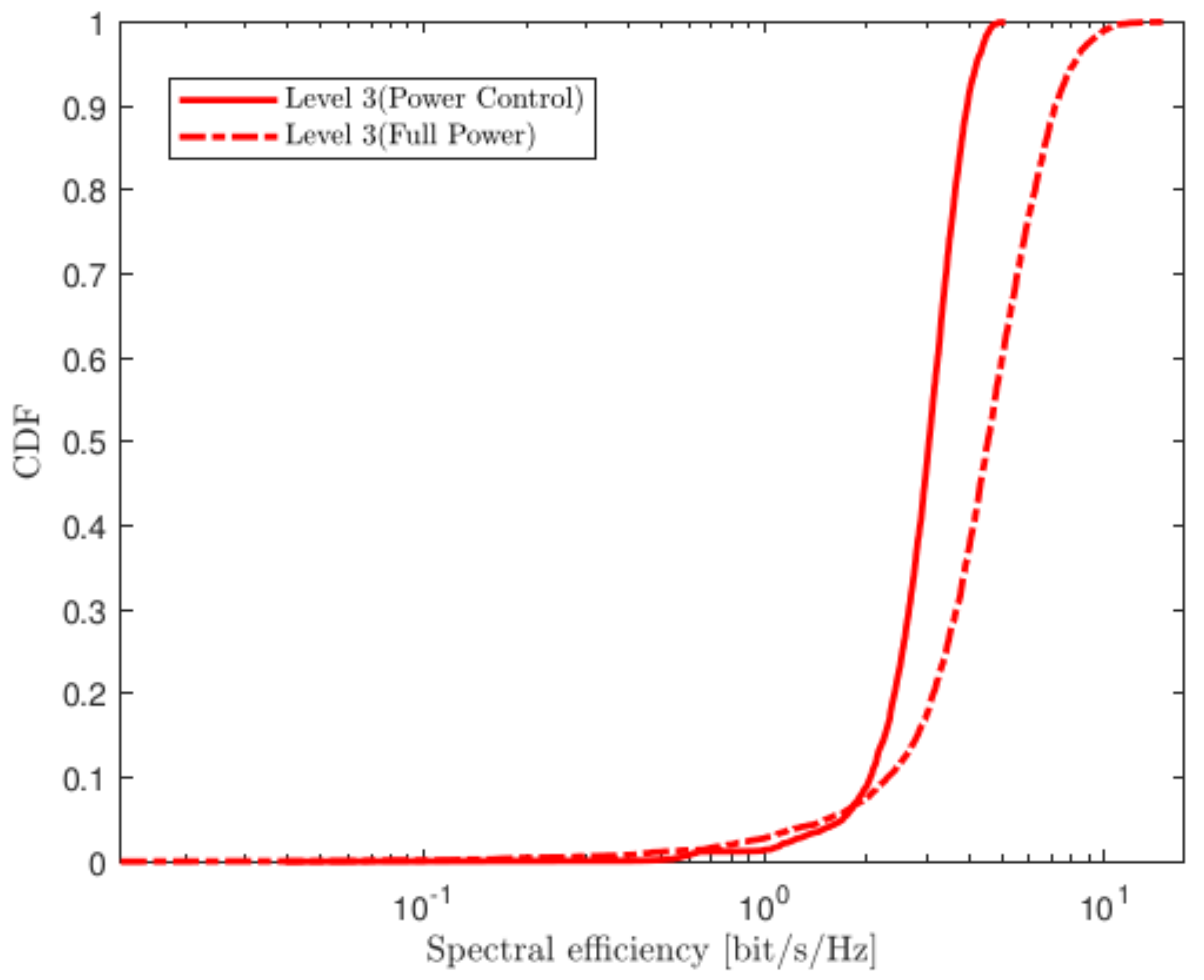
4.2. Power Allocation

A power allocation scheme is considered in [29,39], which is carried out in the uplink transmission phase and only related to statistical CSIs, so it is a feasible scheme for Level 3. The power allocation algorithm can be expressed as:

$$p_k=\frac{\eta }{{\displaystyle \sum _{l\in {\mathcal{Z}}_k^{}}}{\beta }_{kl}}{p}_{max},$$

(31)

where $\eta =\underset{1\le i\le K}{min}{\displaystyle \sum _{l\in {\mathcal{Z}}_i}}{\beta }_{kl}$ and $p_{max}$ denotes the maximum uplink power of each UE. This algorithm is applied to Level 3 and the results are shown in Figure 4.

Figure 4 exposes that Level 3 with power allocation improves the 90%-likely throughput. However, Level 3 with with full power can achieve higher SEs, which means the power allocation algorithm can obtain better SEs of the worst UEs at the expense of total SE loss.

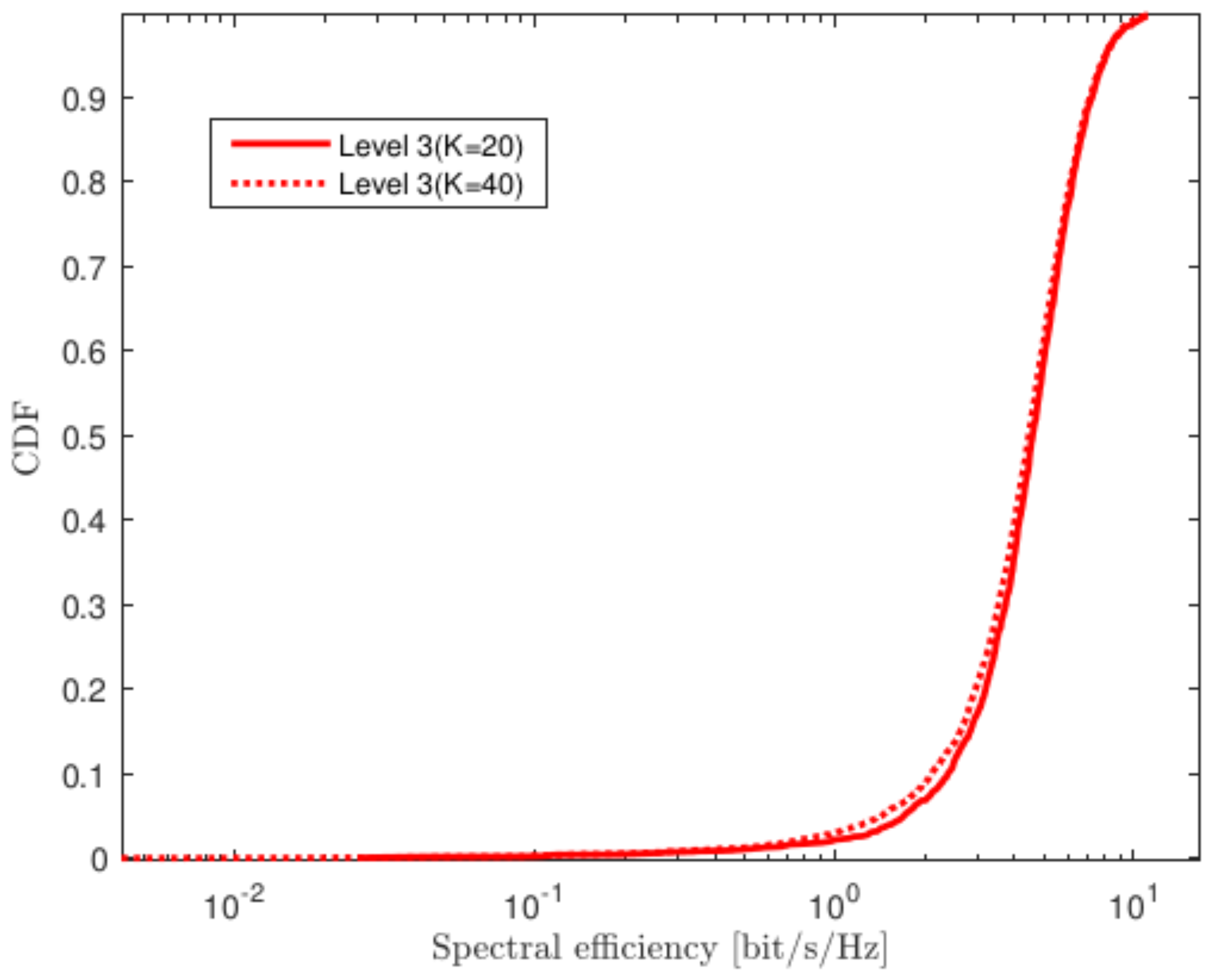
4.3. Varying Numbers of CPUs

Figure 5 plots the CDF of the SEs of Level 3 when varying numbers of CPUs in the VCs. We assume that the total number of APs and CPUs serving for each UE is 24 and $\overline{U}$, respectively. To facilitate calculation, we specify that each CPU provides the same number of APs in the VCs (i.e., when $\overline{U}=3$, 8 APs are selected from the RC of each CPU to associate with the UE.) To satisfy fairness, we shrink the simulation area by 100 times to ensure that each AP can provide the effective signals. The result shows that increasing the number of $\overline{U}$ leads to decreasing the SEs generally, which are caused by reducing the degree of freedom for suppressing the interference in each RC.

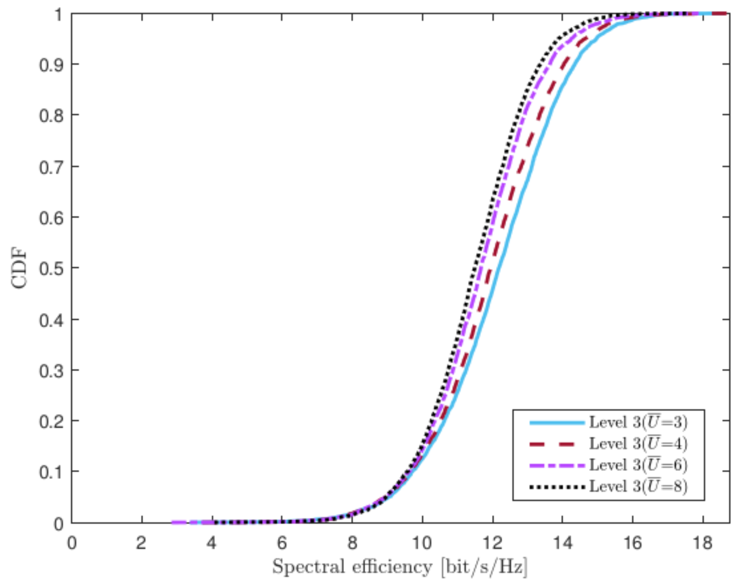
4.4. Varying Numbers of UEs

Figure 6 demonstrates the CDF of the SEs of Level 3 under different numbers of UEs. As can be shown in Figure 6, we can see that the performance of Level 3 only slightly degrades as more UEs are served. It indicates that Level 3 can effectively suppress the interference coming from more UEs.

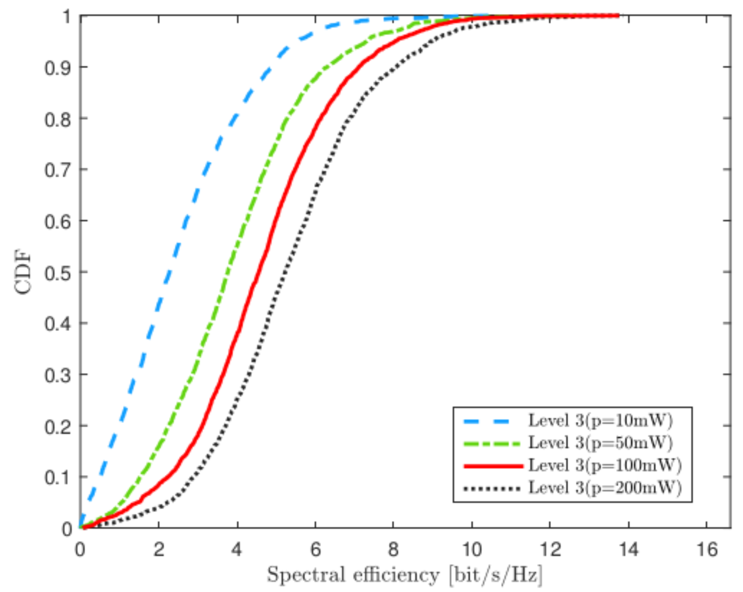
4.5. Varying the Uplink Transmit Power

Figure 7 plots the CDF of the SEs of Level 3 when varying the uplink transmit power for $p_i=p$. Although Level 3 can deal with the interference that comes from UEs, it is greatly affected by the uplink transmit power. The result shows that the performance of Level 3 decreases with the degrades in uplink transmit power.

5. Conclusions

This paper has studied a scalable and user-centric CF-M-MIMO with multiple CPUs. All the APs were divided into several RCs linked to different CPUs and each UE was affiliated with a VC. According to the different degrees of multiple CPUs cooperation, we have derived SE expressions for four different levels of cooperation among multiple CPUs. In particular, we have proposed a low complexity optimization algorithm based on statistical CSI (i.e., Level 3). The results have shown that Level 3 can achieve scalability with lower backhual burden, and the performance loss is negligible compared to Level 4.

References

1. Dai, H.; Molisch, A.F.; Poor, H.V. Downlink capacity of interference-limited MIMO systems with joint detection. IEEE Trans. Wirel. Commun. 2004, 3, 442–453. [Google Scholar] [CrossRef]
2. Choi, W.; Andrews, J.G. Downlink performance and capacity of distributed antenna systems in a multicell environment. IEEE Trans. Wirel. Commun. 2007, 6, 69–73. [Google Scholar] [CrossRef]
3. Andrews, J.G.; Choi, W.; Heath, R.W. Overcoming interference in spatial multiplexing MIMO cellular networks. IEEE Wirel. Commun. Mag. 2007, 14, 95–104. [Google Scholar] [CrossRef]
4. Irmer, R.; Droste, H.; Marsch, P.; Grieger, M.; Fettweis, G.; Brueck, S.; Mayer, H.P.; Thiele, L.; Jungnickel, V. Coordinated multipoint: Concepts, performance, and field trial results. IEEE Commun. Mag. 2011, 49, 102–111. [Google Scholar] [CrossRef] [Green Version]
5. Lozano, A.; Heath, R.W.; Andrews, J.G. Fundamental limits of cooperation. IEEE Trans. Inf. Theory 2013, 59, 5213–5226. [Google Scholar] [CrossRef] [Green Version]
6. Björnson, E.; Kountouris, M.; Debbah, M. Massive MIMO and small cells: Improving energy efficiency by optimal soft-cel coordination. In Proceedings of the 20th International Conference Telecommunication (ICT 2013), Casablanca, Morocco, 6–8 May 2013; pp. 1–5. [Google Scholar]
7. Truong, K.T.; Heath, R.W. The viability of distributed antennas for massive MIMO systems. In Proceedings of the 45nd Asilomar Conference Signals, Systems and Computers, Pacific Grove, CA, USA, 3–6 November 2013; pp. 1318–1323. [Google Scholar]
8. Björnson, E.; Sanguinetti, L.; Hoydis, J.; Debbah, M. Optimal design of energy-efficient multi-user MIMO systems: Is massive MIMO the answer. IEEE Trans. Wirel. Commun. 2015, 14, 3059–3075. [Google Scholar] [CrossRef] [Green Version]
9. Larsson, E.G.; Tufvesson, F.; Edfors, O.; Marzetta, T.L. Massive MIMO for next generation wireless systems. IEEE Commun. Mag. 2014, 52, 186–195. [Google Scholar] [CrossRef] [Green Version]
10. Marzetta, T.L.; Ngo, H.Q. Fundamentals of Massive MIMO; Cambridge University Press: Cambridge, UK, 2016. [Google Scholar]
11. Björnson, E.; Larsson, E.G.; Debbah, M. Massive MIMO for maximal spectral efficiency: How many users and pilots should be allocated? IEEE Trans. Wirel. Commun. 2015, 15, 1293–1308. [Google Scholar] [CrossRef] [Green Version]
12. Ngo, H.Q.; Ashikhmin, A.; Yang, H.; Larsson, E.G.; Marzetta, T.L. Cell-free massive MIMO: Uniformly great service for everyone. In Proceedings of the 2015 IEEE 16th International Workshop on Signal Processing Advances in Wireless Communications (SPAWC), Stockholm, Sweden, 28 June–1 July 2015; pp. 201–205. [Google Scholar]
13. Ngo, H.Q.; Ashikhmin, A.; Yang, H.; Larsson, E.G.; Marzetta, T.L. Cell-free massive MIMO versus small cells. IEEE Trans. Wirel. Commun. 2017, 16, 1834–1850. [Google Scholar] [CrossRef] [Green Version]
14. Interdonato, G.; Björnson, E.; Ngo, H.Q.; Frenger, P.; Larsson, E.G. Ubiquitous cell-free massive MIMO communications. EURASIP J. Wirel. Commun. Netw. 2019, 2019, 197. [Google Scholar] [CrossRef] [Green Version]
15. Zhang, J.; Björnson, E.; Matthaiou, M.; Ng, D.W.K.; Yang, H.; Love, D.J. Prospective Multiple Antenna Technologies for Beyond 5G. IEEE J. Sel. Areas Commun. 2020, 38, 1637–1660. [Google Scholar] [CrossRef]
16. Burr, A.; Bashar, M.; Maryopi, D. Ultra-dense Radio Access Networks for Smart Cities: Cloud-RAN, Fog-RAN and cell-free Massive MIMO. arXiv 2018, arXiv:1811.11077. [Google Scholar]
17. Li, S.; Tolbert, L.M.; Wang, F.; Peng, F.Z. Stray inductance reduction of commutation loop in the P-cell and N-cell-based IGBT phase leg module. IEEE Trans. Power Electron. 2013, 29, 3616–3624. [Google Scholar] [CrossRef]
18. Björnson, E.; Sanguinetti, L. Making cell-free massive MIMO competitive with MMSE processing and centralized implementation. IEEE Trans. Wirel. Commun. 2019, 19, 77–90. [Google Scholar] [CrossRef] [Green Version]
19. Nguyen, L.D.; Duong, T.Q.; Ngo, H.Q.; Tourki, K. Energy efficiency in cell-free massive MIMO with zero-forcing precoding design. IEEE Commun. Lett. 2017, 21, 1871–1874. [Google Scholar] [CrossRef] [Green Version]
20. Björnson, E.; Jorswieck, E. Optimal Resource Allocation in Coordinated Multi-Cell Systems; Now Publishers Inc.: Delft, The Netherlands, 2013. [Google Scholar]
21. Kaltenberger, F.; Jiang, H.; Guillaud, M.; Knopp, R. Relative channel reciprocity calibration in MIMO/TDD systems. In Proceedings of the 2010 Future Network & Mobile Summit, Florence, Italy, 16–18 June 2010; pp. 1–10. [Google Scholar]
22. Zhou, S.; Zhao, M.; Xu, X.; Wang, J.; Yao, Y. Distributed wireless communication system: A new architecture for future public wireless access. IEEE Commun. Mag. 2003, 41, 108–113. [Google Scholar] [CrossRef]
23. Buzzi, S.; D’Andrea, C. Cell-free massive MIMO: User-centric approach. IEEE Commun. Lett. 2017, 6, 706–709. [Google Scholar] [CrossRef]
24. Björnson, E.; Hoydis, J.; Sanguinetti, L. Massive MIMO networks: Spectral, energy, and hardware efficiency. Found. Trends Signal Process. 2017, 11, 154–655. [Google Scholar] [CrossRef]
25. Sanguinetti, L.; Björnson, E.; Hoydis, J. Toward massive MIMO 2.0: Understanding spatial correlation, interference suppression, and pilot contamination. IEEE Trans. Commun. 2019, 68, 232–257. [Google Scholar] [CrossRef] [Green Version]
26. Björnson, E.; Sanguinetti, L. Scalable cell-free massive MIMO systems. IEEE Trans. Commun. 2020, 68, 4247–4261. [Google Scholar] [CrossRef] [Green Version]
27. Zhang, J.; Zhang, J.; Björnson, E.; Ai, B. Local partial zero-forcing combining for cell-free massive MIMO systems. IEEE Trans. Commun. 2021, 69, 8459–8473. [Google Scholar] [CrossRef]
28. Interdonato, G.; Buzzi, S. Conjugate beamforming with fractional-exponent normalization and scalable power control in cell-free massive MIMO. In Proceedings of the 2021 IEEE 22nd International Workshop on Signal Processing Advances in Wireless Communications (SPAWC), Lucca, Italy, 27–30 September 2021; pp. 396–400. [Google Scholar]
29. Nikbakht, R.; Mosayebi, R.; Lozano, A. Uplink fractional power control and downlink power allocation for cell-free networks. IEEE Wirel. Commun. Lett. 2020, 9, 774–777. [Google Scholar] [CrossRef]
30. Interdonato, G.; Karlsson, M.; Björnson, E.; Larsson, E.G. Local partial zero-forcing precoding for cell-free massive MIMO. IEEE Trans. Wirel. Commun. 2020, 19, 4758–4774. [Google Scholar] [CrossRef] [Green Version]
31. Interdonato, G.; Frenger, P.; Larsson, E.G. Scalability aspects of cell-free massive MIMO. In Proceedings of the ICC 2019—2019 IEEE International Conference on Communications (ICC), Shanghai, China, 20–24 May 2019; pp. 1–6. [Google Scholar]
32. Nayebi, E.; Ashikhmin, A.; Marzetta, T.L.; Yang, H.; Rao, B.D. Precoding and power optimization in cell-free massive MIMO systems. IEEE Trans. Wirel. Commun. 2017, 16, 4445–4459. [Google Scholar] [CrossRef]
33. Nayebi, E.; Ashikhmin, A.; Marzetta, T.L.; Rao, B.D. Performance of cell-free massive MIMO systems with MMSE and LSFD receivers. In Proceedings of the 2016 50th Asilomar Conference on Signals, Systems and Computers, Pacific Grove, CA, USA, 6–9 November 2016; pp. 203–207. [Google Scholar]
34. Riera-Palou, F.; Femenias, G. Decentralization issues in cell-free massive MIMO networks with zero-forcing precoding. In Proceedings of the 2019 57th Annual Allerton Conference on Communication, Control, and Computing (Allerton), Monticello, IL, USA, 24–27 September 2019; pp. 521–527. [Google Scholar]
35. Aguerri, I.E.; Zaidi, A.; Caire, G.; Shitz, S.S. On the capacity of cloud radio access networks with oblivious relaying. IEEE Trans. Inf. Theory 2019, 65, 4575–4596. [Google Scholar] [CrossRef] [Green Version]
36. Biglieri, E.; Proakis, J.; Shamai, S. Fading channels: Information-theoretic and communications aspects. IEEE Trans. Inf. Theory 1998, 44, 2619–2692. [Google Scholar] [CrossRef]
37. Ngo, H.Q.; Tataria, H.; Matthaiou, M.; Jin, S.; Larsson, E.G. On the performance of cell-free massive MIMO in Ricean fading. In Proceedings of the 2018 52nd Asilomar Conference on Signals, Systems, and Computers, Pacific Grove, CA, USA, 28–31 October 2018; pp. 980–984. [Google Scholar]
38. Adhikary, A.; Ashikhmin, A.; Marzetta, T.L. Uplink interference reduction in large-scale antenna systems. IEEE Trans. Commun. 2017, 65, 2194–2206. [Google Scholar] [CrossRef]
39. Nikbakht, R.; Lozano, A. Uplink fractional power control for cell-free wireless networks. In Proceedings of the ICC 2019—2019 IEEE International Conference on Communications (ICC), Shanghai, China, 20–24 May 2019; pp. 1–5. [Google Scholar]
Figure 1. Example of virtual clusters in the CF-M-MIMO with multiple CPUs. The yellow area, red area and blue area represent virtual cluster, real cluster and the intersection of virtual cluster and real cluster, respectively.
Mathematics 10 01900 g001
Figure 2. Comparison of CF-M-MIMO with different levels of multiple CPUs cooperation in the case that partial APs serve the UEs.
Mathematics 10 01900 g002
Figure 3. Comparison of CF-M-MIMO with different levels of multiple CPUs cooperation in the case that all APs serve the UEs.
Mathematics 10 01900 g003
Figure 4. In the case that partial APs serve the UEs, the SE comparison of Level 3 between full power and power allocation.
Mathematics 10 01900 g004
Figure 5. When the total number of APs is fixed, the SE comparison of different number of CPUs.
Mathematics 10 01900 g005
Figure 6. The SE comparison of different number of UEs.
Mathematics 10 01900 g006
Figure 7. The SE comparison under different uplink transmit power.
Mathematics 10 01900 g007