Epidemic Dynamics of Two-Pathogen Spreading for Pairwise Models

Abstract

In the real world, pathogens do not exist in isolation. The transmission of one pathogen may be affected by the presence of other pathogens, and certain pathogens generate multiple strains with different spreading features. Hence, the behavior of multi-pathogen transmission has attracted much attention in epidemiological research. In this paper, we use the pairwise approximation method to formulate two-pathogen models capturing cross-immunity, super-infection, and co-infection phenomena, in which each pathogen follows a susceptible-infected-susceptible (SIS) mechanism. For each model, we calculate the basic reproduction number and analyze the stability of equilibria, and discuss the differences from the mean-field approach. We demonstrate that simulations are in good agreement with the analytical results.

1. Introduction

Epidemic diseases have been a great threat throughout human history. Examples of these ancestral enemies include dengue fever [1], severe acute respiratory syndrome (SARS) [2,3], tuberculosis (TB) [4], and swine-origin influenza A (H1N1) [5]. During disease propagation, infections of different pathogens may impact each other. Furthermore, a single pathogen always generates many strains with different spreading features. Hence, an important issue in current epidemiological research is the behavior of multi-pathogens. The majority of existing work focuses on cross-immunity and competing pathogens [6,7,8]. In this case, multiple pathogens compete for the same host, and a host infected by one disease will have increased immunity to another. For example, the human immunodeficiency virus (HIV) has many genetic varieties, and can be divided into several different strains, such as HIV-1 and HIV-2, which provide cross-immunity [9]. However, there are forms of interaction between two pathogens other than cross-immunity, including super-infection, where one more virulent pathogen can out-compete the other less virulent pathogen at the level of intra-host competition [10,11]; or co-infection [12,13,14], in which two pathogens can be hosted in one individual. 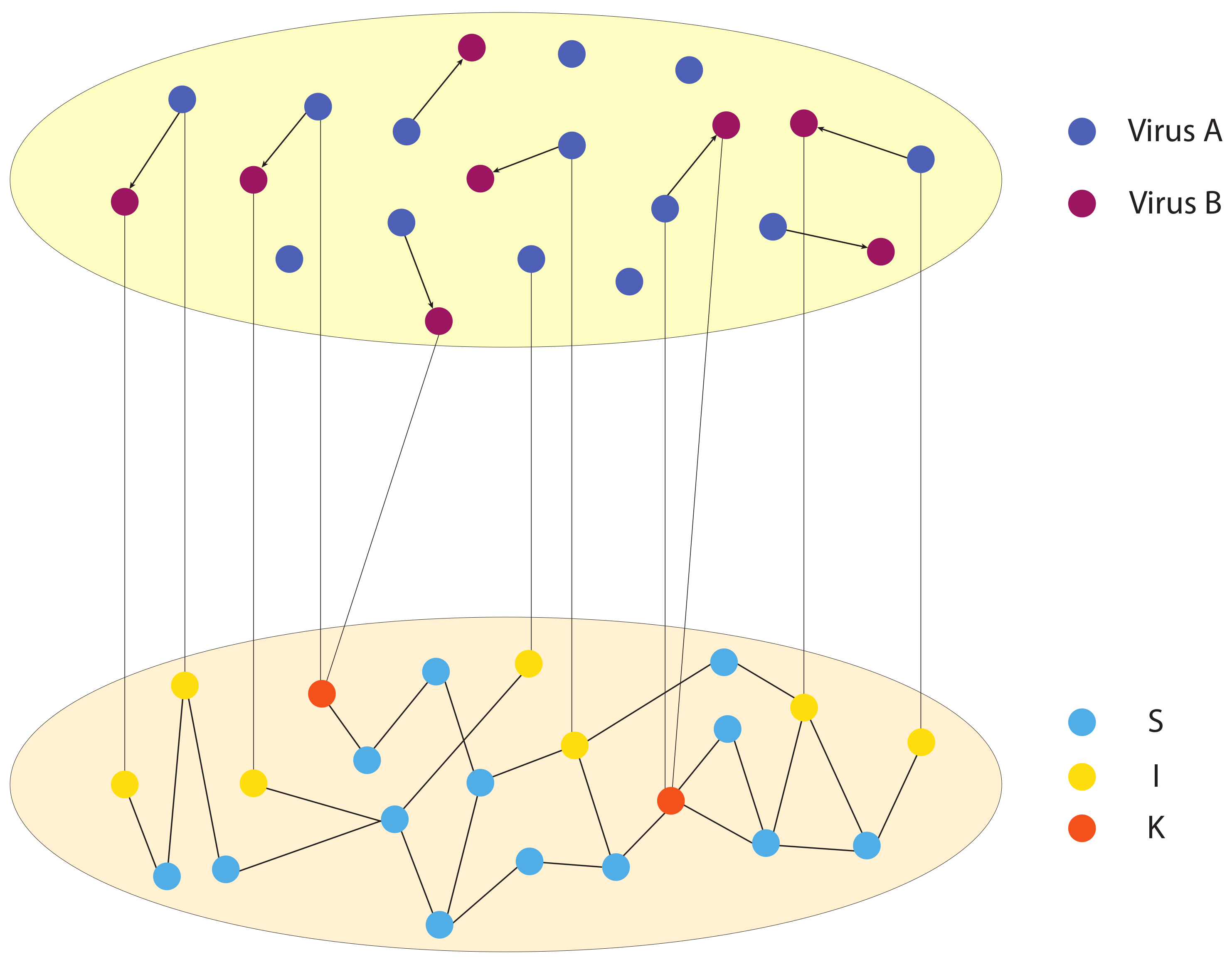For example, COVID-19 has multiple SARS-CoV-2 haplotypes [15]. As Figure 1 illustrates, one person can be infected by one virus, or two viruses in sequence; one virus can evolve into another virus; and one person can be infected by another person with two viruses.

Existing work on the spreading of multiple super-infection and co-infection pathogens is limited. Differential equation models are a useful tool in investigating and predicting the dynamical behavior of epidemic spreading. Most of these models are based on the assumption of a randomly mixing population, where contacts between any two individuals (nodes) are equally likely. However, in many cases the assumption of a randomly mixing population can be unrealistic. Disease transmission in many epidemic systems can be represented as a graph where vertices denote individuals, and edges connecting a pair of vertices indicate interactions between individuals. It is obvious that only when the susceptible vertices (S) and the infected vertices (I) form a pair (a connection between S and I) can infection occur. For example, if we consider sexually transmitted diseases and ignore all spread by non-sexual means, connections are only between people that have sexual contact with each other. Hence, mean-field models constructed at the single node level cannot capture the vital spatial structure of the network.

The key insight to capturing spatial information is to track pairs rather than individuals [12,16,17,18,19,20,21,22,23,24,25,26]. Altmann first formulated a partner model to investigate the sexual disease and inferred the basic reproduction number based on a Markov process [16]. Keeling and Rand formulated a correlation model to study measles [17], and Morris put forward the corresponding pair approximation method and estimated the error [18]. More recently, Sharkey investigated the asymmetric pair-level model on a directed network, and provided the asymmetric pair-level closure approximation [19]. In 2007, Trapman formulated a pair approximation method and discussed problems inherent to this approach. They also defined a new reproduction number similar to the basic reproduction number $R_0$ [20]. By comparing the impact of regular and random contacts, Eames found that disease spreads faster and further when contacts are random, especially in highly clustered populations [21]. In all, the idea of a pair approximation method on a homogeneous network is basically the same as the idea behind randomly mixing populations, but here the pairs of connected individuals are randomly mixing instead of the single individuals.

In this paper, we study three two-pathogen epidemic models with the pairwise method. All models follow a susceptible-infected-susceptible (SIS) process. In Section 2, we formulate two-pathogen models in which pathogen interactions correspond to cross-immunity, super-infection or co-infection. We calculate the basic reproduction number for each model, and show the differences from the value calculated using the traditional mean-field method. In Section 3, we validate each model via comparison with numerical simulations on networks. Finally, some remarks and conclusions are given in Section 4.

2. Models and Their Epidemic Thresholds

In this section, we introduce the two-pathogen models in cross-immunity infection, then give the super-infection or co-infection forms. We calculate the basic reproduction numbers for each model and compare them with those calculated using the traditional mean-field method.

Flowcharts of two-pathogen disease transmission with cross-immunity infection, super-infection, and co-infection forms are given in Figure 2, and notation and parameters are listed in

Table 1. Notation used in models.

Symbol	Meaning
$\left[S\right]$	The total number of susceptible nodes in the network
$\left[I_1\right]$	The total number of nodes infected by pathogen 1 in the network
$\left[I_2\right]$	The total number of nodes infected by pathogen 2 in the network
$\left[AB\right]$	The number of two-tuples composed of connected nodes in state A and a node in state B
$\left[ABC\right]$	The number of connected triples comprising a node in state A, a node in state B, and a node in state C
$[A_1\dots A_q]$	The number of q-tuples (q connected nodes in a path of length $q-1$) comprising a sequence of nodes in the states $A_1,\dots ,A_q$
$C_{AB}$	$C_{AB}=\frac{N\left[AB\right]}{n\left[A\right]\left[B\right]}$, the correlation coefficient between state A and B
${\lambda }_k$	The spreading rate of pathogen k, $k=1,2$
${\lambda }_k^{\prime }$	The super-spreading rate at which a node becomes infected by pathogen k when it is already infected with the other pathogen, $k=1,2$
${\gamma }_k$	The recovery rate of pathogen k to state S, $k=1,2$
${\gamma }_k^{\prime }$	The recovery rate from the two-pathogen state K to state $I_k$, $k=1,2$
${\gamma }_3$	The recovery rate to state S for both pathogen 1 and 2
n	The average degree of a vertice in the network
N	The size of the network

.

2.1. Cross-Immunity Infection Pathogens

In the cross-immunity form of pathogen interaction, two pathogens compete for one host. If an individual is infected by pathogen 1, it will be immune to pathogen 2. Using the traditional mean-field approach, we can formulate the model as follows:

$$\left\{\begin{array}{c}\frac{d\left[S\right]}{dt}=-n{\lambda }_1\left[S\right]\left[I_1\right]/N-n{\lambda }_2\left[S\right]\left[I_2\right]/N+{\gamma }_1\left[I_1\right]+{\gamma }_2\left[I_2\right]\hfill \\ \frac{d\left[I_1\right]}{dt}=n{\lambda }_1\left[S\right]\left[I_1\right]/N-{\gamma }_1\left[I_1\right]\hfill \\ \frac{d\left[I_2\right]}{dt}=n{\lambda }_2\left[S\right]\left[I_2\right]/N-{\gamma }_2\left[I_2\right]\hfill \end{array}\right.$$

(1)

Following [18,27,28], a pairwise method can be applied to formulate the competing form. The infection occurs only if there is a pair (edge) between a susceptible individual and an infected individual. The authors of [29] provide a pairwise model of two cross-immunity pathogens with rewiring on a regular or random network. In the absence of rewiring, differential equations can be formulated as follows:

$$\left\{\begin{array}{c}\frac{d\left[S\right]}{dt}=-{\lambda }_1\left[S{I}_1\right]-{\lambda }_2\left[S{I}_2\right]+{\gamma }_1\left[I_1\right]+{\gamma }_2\left[I_2\right]\hfill \\ \frac{d\left[I_1\right]}{dt}={\lambda }_1\left[S{I}_1\right]-{\gamma }_1\left[I_1\right]\hfill \\ \frac{d\left[I_2\right]}{dt}={\lambda }_2\left[S{I}_2\right]-{\gamma }_2\left[I_2\right]\hfill \end{array}\right.$$

(2)

Because infection spreads from infected nodes to susceptible nodes, the governing equation for node state $\left[A\right]$ contains terms of the form $\left[AB\right]$, representing counts of two-tuples. Similarly, the evolution of two-tuples depends on triples (three-tuples) and, more generally, the governing equation of q-tuples will involve $(q+1)$-tuples. Therefore, without approximation, the system comprises an infinite-dimensional set. To allow for a solution, we need to find an approximation which allows us to truncate the set of equations at some point—i.e., to close the system—in a process called moment closure. We consider a method of moment closure called pair approximation.

The above system of differential equations, with $\left[S{I}_1\right]$ and $\left[S{I}_2\right]$ on the right-hand side, but without governing equations for $\left[S{I}_1\right]$ and $\left[S{I}_2\right]$, are not closed. We express the dynamics of these counts of two-tuples $\left[AB\right]$ in terms of counts of triples $\left[CDE\right]$:

$$\left\{\begin{array}{c}\frac{d\left[SS\right]}{dt}=-2{\lambda }_1\left[SS{I}_1\right]-2{\lambda }_2\left[SS{I}_2\right]+2{\gamma }_1\left[S{I}_1\right]+2{\gamma }_2\left[S{I}_2\right]\hfill \\ \frac{d\left[S{I}_1\right]}{dt}={\lambda }_1\left[SS{I}_1\right]-{\gamma }_1\left[S{I}_1\right]+{\gamma }_1\left[I_1{I}_1\right]+{\gamma }_2\left[I_1{I}_2\right]-{\lambda }_1\left[S{I}_1\right]-{\lambda }_1\left[I_{1}S{I}_1\right]-{\lambda }_2\left[I_{1}S{I}_2\right]\hfill \\ \frac{d\left[S{I}_2\right]}{dt}={\lambda }_2\left[SS{I}_2\right]-{\gamma }_2\left[S{I}_2\right]+{\gamma }_1\left[I_1{I}_2\right]+{\gamma }_2\left[I_2{I}_2\right]-{\lambda }_2\left[S{I}_2\right]-{\lambda }_1\left[I_{1}S{I}_2\right]-{\lambda }_2\left[I_{2}S{I}_2\right]\hfill \\ \frac{d\left[I_1{I}_1\right]}{dt}=-2{\gamma }_1\left[I_1{I}_1\right]+2{\lambda }_1\left[S{I}_1\right]+2{\lambda }_1\left[I_{1}S{I}_1\right]\hfill \\ \frac{d\left[I_1{I}_2\right]}{dt}=-{\gamma }_1\left[I_1{I}_2\right]-{\gamma }_2\left[I_1{I}_2\right]+{\lambda }_1\left[I_{1}S{I}_2\right]+{\lambda }_2\left[I_{1}S{I}_2\right]\hfill \\ \frac{d\left[I_2{I}_2\right]}{dt}=-2{\gamma }_2\left[I_2{I}_2\right]+2{\lambda }_2\left[S{I}_2\right]+2{\lambda }_2\left[I_{2}S{I}_2\right]\hfill \end{array}\right.$$

(3)

In these equations, triples appear on the right-hand side, so that the system still is not closed. To close the system, the number of triples in certain states will be approximated by the number of pairs [20]. On a homogeneous network, such as an ER random graph, the degree distribution is similar to Poisson distribution, meaning that the degrees of most nodes are near the mean degree n. Assuming that the state of the third individual in the triple only depends on the state of the second individual [18,28], the number of triples $\left[ABC\right]$ can be approximated as the product of: (1) the number of two-tuples involving a node in state A and a node in state B, $\left[AB\right]$; (2) the expected number of neighbors in the C state of a node in the $\left[B\right]$ state: $\frac{\left[BC\right]}{\left[B\right]}$; and (3) a factor $p=\frac{n}{n-1}$, which corrects for the fact that one of the n links in which the node in state B connects with a node in state A and so cannot connect with a node in state C. Therefore the approximation for the number of triples is (full details in [18,28]):

$$\left[ABC\right]\approx p\frac{\left[AB\right]\left[BC\right]}{\left[B\right]}$$

(4)

Using Equation (4), we can close the pairwise differential Equation (3) to obtain the following equivalent equations:

$$\left\{\begin{array}{c}\frac{d\left[I_1\right]}{dt}={\lambda }_1\left[S{I}_1\right]-{\gamma }_1\left[I_1\right]\hfill \\ \frac{d\left[I_2\right]}{dt}={\lambda }_2\left[S{I}_2\right]-{\gamma }_2\left[I_2\right]\hfill \\ \frac{d\left[S{I}_1\right]}{dt}=-({\lambda }_1+{\gamma }_1)\left[S{I}_1\right]+{\gamma }_1\left[I_1{I}_1\right]+{\gamma }_2\left[I_1{I}_2\right]+{\lambda }_{1}p\frac{\left[SS\right]\left[S{I}_1\right]}{\left[S\right]}-{\lambda }_{1}p\frac{{\left[S{I}_1\right]}^2}{\left[S\right]}-{\lambda }_{2}p\frac{\left[S{I}_1\right]\left[S{I}_2\right]}{\left[S\right]}\hfill \\ \frac{d\left[S{I}_2\right]}{dt}=-({\lambda }_2+{\gamma }_2)\left[S{I}_2\right]+{\gamma }_1\left[I_1{I}_2\right]+{\gamma }_2\left[I_2{I}_2\right]+{\lambda }_{2}p\frac{\left[SS\right]\left[S{I}_2\right]}{\left[S\right]}-{\lambda }_{2}p\frac{{\left[S{I}_2\right]}^2}{\left[S\right]}-{\lambda }_{1}p\frac{\left[S{I}_1\right]\left[S{I}_2\right]}{\left[S\right]}\hfill \\ \frac{d\left[I_1{I}_1\right]}{dt}=2{\lambda }_1\left[S{I}_1\right]-2{\gamma }_1\left[I_1{I}_1\right]+2{\lambda }_{1}p\frac{{\left[S{I}_1\right]}^2}{\left[S\right]}\hfill \\ \frac{d\left[I_1{I}_2\right]}{dt}=-({\gamma }_1+{\gamma }_2)\left[I_1{I}_2\right]+{\lambda }_{1}p\frac{\left[S{I}_1\right]\left[S{I}_2\right]}{\left[S\right]}+{\lambda }_{2}p\frac{\left[S{I}_1\right]\left[S{I}_2\right]}{\left[S\right]}\hfill \\ \frac{d\left[I_2{I}_2\right]}{dt}=2{\lambda }_2\left[S{I}_2\right]-2{\gamma }_2\left[I_2{I}_2\right]+2{\lambda }_{2}p\frac{{\left[S{I}_2\right]}^2}{\left[S\right]}\hfill \end{array}\right.$$

(5)

with the total counts of nodes and two-tuples satisfying:

$$N=\left[S\right]+\left[I_1\right]+\left[I_2\right],nN=\left[SS\right]+2\left[S{I}_1\right]+2\left[S{I}_2\right]+\left[I_1{I}_1\right]+2\left[I_1{I}_2\right]+\left[I_2{I}_2\right]$$

Since N is the number of individuals, and n is the mean degree, the number of two-tuples is $nN$.

Now, we study the stability of the disease-free equilibrium. Following [29], we obtain the characteristic equation of the cross-immunity two-pathogen model Equation (5). The Jacobian matrix of the infected part of Equation (5) at the disease-free equilibrium (where $\left[S\right]=N,\left[SS\right]=nN$, and other infected individuals and pairs are equal to zero) is:

$$A=\left[\begin{array}{ccccccc}-{\gamma }_1& 0& {\lambda }_1& 0& 0& 0& 0\\ 0& -{\gamma }_2& 0& {\lambda }_2& 0& 0& 0\\ 0& 0& -({\lambda }_1+{\gamma }_1)+{\lambda }_{1}pn& 0& {\gamma }_1& {\gamma }_2& 0\\ 0& 0& 0& -({\lambda }_2+{\gamma }_2)+{\lambda }_{2}pn& 0& {\gamma }_1& {\gamma }_2\\ 0& 0& 2{\lambda }_1& 0& -2{\gamma }_1& 0& 0\\ 0& 0& 0& 0& 0& -({\gamma }_1+{\gamma }_2)& 0\\ 0& 0& 0& 2{\lambda }_2& 0& 0& -2{\gamma }_2\end{array}\right]$$

The disease-free equilibrium will be stable as long as all eigenvalues $\mu$ of A are negative, but if any eigenvalues have a positive real part, then this equilibrium cannot be stable. Let E denote the identity matrix. The characteristic equation $|A-\mu E|=0$ is:

$$\begin{array}{cc}\hfill a·[{\mu }^2-({\lambda }_{1}pn-{\lambda }_1-3{\gamma }_1)\mu +& 2{\gamma }_1^2-2{\lambda }_1{\gamma }_{1}pn]\hfill \\ \hfill & ·[{\mu }^2-({\lambda }_{2}pn-{\lambda }_2-3{\gamma }_2)\mu +2{\gamma }_2^2-2{\lambda }_2{\gamma }_{2}pn]=0\hfill \end{array}$$

(6)

where $a=({\gamma }_1+\mu )·({\gamma }_2+\mu )·({\gamma }_1+{\gamma }_2+\mu )$. All the eigenvalues of Equation (6) are negative when the constant terms in the final two quadratic factors are positive, i.e., when $2{\gamma }_1^2-2{\lambda }_1{\gamma }_{1}pn>0$ and $2{\gamma }_2^2-2{\lambda }_2{\gamma }_{2}pn>0$ or, equivalently, when $\frac{{\lambda }_1(n-1)}{{\gamma }_1},\frac{{\lambda }_2(n-1)}{{\gamma }_2}<1$. Based on this condition, we infer the basic reproduction number $R_0$ as:

$$R_0=max\left\{\frac{{\lambda }_1(n-1)}{{\gamma }_1},\frac{{\lambda }_2(n-1)}{{\gamma }_2}\right\}$$

From this analysis, we obtain the following theorem.

Theorem 1.

If $R_0<1$, then the system (5) has a unique disease-free equilibrium and is locally asymptotically stable; it is unstable if $R_0\ge 1$.

In comparison, a calculation with the mean-field equation, Equation (1), would yield a slightly larger value for the basic reproduction number, $R_0=max\left\{\frac{n{\lambda }_1}{{\gamma }_1},\frac{n{\lambda }_2}{{\gamma }_2}\right\}$.

2.2. Super-Infection Pathogens

As in the cross–immunity infection case, under super-infection both viruses cannot coexist in a single host. The individual’s states are divided into susceptible, infected state 1, and infected state 2, respectively. Infected states 1 and 2 represent different strains and have transmission rates ${\lambda }_1$ and ${\lambda }_2$, respectively. Infected persons in state 1 are transformed into infected persons in state 2 at rate ${\lambda }_2^{\prime }$, but the reverse transformation is not possible. The mean-field equation can be written:

$$\left\{\begin{array}{c}\frac{d\left[S\right]}{dt}=-n{\lambda }_1\left[S\right]\left[I_1\right]/N-n{\lambda }_2\left[S\right]\left[I_2\right]/N+{\gamma }_1\left[I_1\right]+{\gamma }_2\left[I_2\right]\hfill \\ \frac{d\left[I_1\right]}{dt}=n{\lambda }_1\left[S\right]\left[I_1\right]/N-{\gamma }_1\left[I_1\right]-n{\lambda }_2^{\prime }\left[I_1\right]\left[I_2\right]/N\hfill \\ \frac{d\left[I_2\right]}{dt}=n{\lambda }_2\left[S\right]\left[I_2\right]/N-{\gamma }_2\left[I_2\right]+n{\lambda }_2^{\prime }\left[I_1\right]\left[I_2\right]/N\hfill \end{array}\right.$$

(7)

Similarly to Section 2.1, the pairwise equations of super-infection pathogens can be formulated as:

$$\left\{\begin{array}{c}\frac{d\left[S\right]}{dt}=-{\lambda }_1\left[S{I}_1\right]-{\lambda }_2\left[S{I}_2\right]+{\gamma }_1\left[I_1\right]+{\gamma }_2\left[I_2\right]\hfill \\ \frac{d\left[I_1\right]}{dt}={\lambda }_1\left[S{I}_1\right]-{\gamma }_1\left[I_1\right]-{\lambda }_2^{\prime }\left[I_1{I}_2\right]\hfill \\ \frac{d\left[I_2\right]}{dt}={\lambda }_2\left[S{I}_2\right]-{\gamma }_2\left[I_2\right]+{\lambda }_2^{\prime }\left[I_1{I}_2\right]\hfill \\ \frac{d\left[SS\right]}{dt}=-2{\lambda }_1\left[SS{I}_1\right]-2{\lambda }_2\left[SS{I}_2\right]+2{\gamma }_1\left[S{I}_1\right]+2{\gamma }_2\left[S{I}_2\right]\hfill \\ \frac{d\left[S{I}_1\right]}{dt}={\lambda }_1\left[SS{I}_1\right]-{\gamma }_1\left[S{I}_1\right]+{\gamma }_1\left[I_1{I}_1\right]+{\gamma }_2\left[I_1{I}_2\right]-{\lambda }_1\left[S{I}_1\right]-{\lambda }_1\left[I_{1}S{I}_1\right]-{\lambda }_2\left[I_{1}S{I}_2\right]-{\lambda }_2^{\prime }\left[S{I}_1{I}_2\right]\hfill \\ \frac{d\left[S{I}_2\right]}{dt}={\lambda }_2\left[SS{I}_2\right]-{\gamma }_2\left[S{I}_2\right]+{\gamma }_1\left[I_1{I}_2\right]+{\gamma }_2\left[I_2{I}_2\right]-{\lambda }_2\left[S{I}_2\right]-{\lambda }_1\left[I_{1}S{I}_2\right]-{\lambda }_2\left[I_{2}S{I}_2\right]+{\lambda }_2^{\prime }\left[S{I}_1{I}_2\right]\hfill \\ \frac{d\left[I_1{I}_1\right]}{dt}=-2{\gamma }_1\left[I_1{I}_1\right]+2{\lambda }_1\left[S{I}_1\right]+2{\lambda }_1\left[I_{1}S{I}_1\right]-2{\lambda }_2^{\prime }\left[I_1{I}_1{I}_2\right]\hfill \\ \frac{d\left[I_1{I}_2\right]}{dt}=-{\gamma }_1\left[I_1{I}_2\right]-{\gamma }_2\left[I_1{I}_2\right]+{\lambda }_1\left[I_{1}S{I}_2\right]+{\lambda }_2\left[I_{1}S{I}_2\right]-{\lambda }_2^{\prime }\left[I_1{I}_2\right]-{\lambda }_2^{\prime }\left[I_2{I}_1{I}_2\right]+{\lambda }_2^{\prime }\left[I_1{I}_1{I}_2\right]\hfill \\ \frac{d\left[I_2{I}_2\right]}{dt}=-2{\gamma }_2\left[I_2{I}_2\right]+2{\lambda }_2\left[S{I}_2\right]+2{\lambda }_2\left[I_{2}S{I}_2\right]+2{\lambda }_2^{\prime }\left[I_2{I}_1{I}_2\right]+2{\lambda }_2^{\prime }\left[I_1{I}_2\right]\hfill \end{array}\right.$$

(8)

Once again, we use the approximation of Equation (4) to close the triples on the right-hand-side. To derive the basic reproduction number, we focus on the terms involving infection:

$$\left\{\begin{array}{c}\frac{d\left[I_1\right]}{dt}={\lambda }_1\left[S{I}_1\right]-{\gamma }_1\left[I_1\right]-{\lambda }_2^{\prime }\left[I_1{I}_2\right]\hfill \\ \frac{d\left[I_2\right]}{dt}={\lambda }_2\left[S{I}_2\right]-{\gamma }_2\left[I_2\right]+{\lambda }_2^{\prime }\left[I_1{I}_2\right]\hfill \\ \frac{d\left[S{I}_1\right]}{dt}=-({\lambda }_1+{\gamma }_1)\left[S{I}_1\right]+{\gamma }_1\left[I_1{I}_1\right]+{\gamma }_2\left[I_1{I}_2\right]+{\lambda }_{1}p\frac{\left[SS\right]\left[S{I}_1\right]}{\left[S\right]}-{\lambda }_{1}p\frac{{\left[S{I}_1\right]}^2}{\left[S\right]}-{\lambda }_{2}p\frac{\left[S{I}_1\right]\left[S{I}_2\right]}{\left[S\right]}-{\lambda }_2^{\prime }p\frac{\left[S{I}_1\right]\left[I_1{I}_2\right]}{\left[I_1\right]}\hfill \\ \frac{d\left[S{I}_2\right]}{dt}=-({\lambda }_2+{\gamma }_2)\left[S{I}_2\right]+{\gamma }_1\left[I_1{I}_2\right]+{\gamma }_2\left[I_2{I}_2\right]+{\lambda }_{2}p\frac{\left[SS\right]\left[S{I}_2\right]}{\left[S\right]}-{\lambda }_{2}p\frac{{\left[S{I}_2\right]}^2}{\left[S\right]}-{\lambda }_{1}p\frac{\left[S{I}_1\right]\left[S{I}_2\right]}{\left[S\right]}+{\lambda }_2^{\prime }p\frac{\left[S{I}_1\right]\left[I_1{I}_2\right]}{\left[I_1\right]}\hfill \\ \frac{d\left[I_1{I}_1\right]}{dt}=2{\lambda }_1\left[S{I}_1\right]-2{\gamma }_1\left[I_1{I}_1\right]+2{\lambda }_{1}p\frac{{\left[S{I}_1\right]}^2}{\left[S\right]}-{\lambda }_2^{\prime }p\frac{\left[I_1{I}_1\right]\left[I_1{I}_2\right]}{\left[I_1\right]}\hfill \\ \frac{d\left[I_1{I}_2\right]}{dt}=-({\gamma }_1+{\gamma }_2+{\lambda }_2^{\prime })\left[I_1{I}_2\right]+{\lambda }_{1}p\frac{\left[S{I}_1\right]\left[S{I}_2\right]}{\left[S\right]}+{\lambda }_{2}p\frac{\left[S{I}_1\right]\left[S{I}_2\right]}{\left[S\right]}-{\lambda }_2^{\prime }p\frac{{\left[I_1{I}_2\right]}^2}{\left[I_1\right]}+{\lambda }_2^{\prime }p\frac{\left[I_1{I}_1\right]\left[I_1{I}_2\right]}{\left[I_1\right]}\hfill \\ \frac{d\left[I_2{I}_2\right]}{dt}=2{\lambda }_2\left[S{I}_2\right]+2{\lambda }_2^{\prime }\left[I_1{I}_2\right]-2{\gamma }_2\left[I_2{I}_2\right]+2{\lambda }_{2}p\frac{{\left[S{I}_2\right]}^2}{\left[S\right]}+2{\lambda }_2^{\prime }p\frac{{\left[I_1{I}_2\right]}^2}{\left[I_1\right]}\hfill \end{array}\right.$$

(9)

with the total counts of nodes and two-tuples satisfying:

$$N=\left[S\right]+\left[I_1\right]+\left[I_2\right],nN=\left[SS\right]+2\left[S{I}_1\right]+2\left[S{I}_2\right]+\left[I_1{I}_1\right]+2\left[I_1{I}_2\right]+\left[I_2{I}_2\right]$$

Theorem 2.

For the super-infection two-pathogen model, let:

$$R_0=max\left\{\frac{{\lambda }_1(n-1)}{{\gamma }_1},\frac{{\lambda }_2(n-1)}{{\gamma }_2}\right\}$$

If $R_0<1$, then the system (9) has a unique disease-free equilibrium and is locally asymptotically stable; if $R_0\ge 1$, it is unstable.

Proof. 

Near the disease-free equilibrium, $\frac{\left[II\right]}{\left[I\right]}=\frac{n{C}_{II}\left[I\right]}{N}\approx 0$ and $\frac{\left[S{I}_i\right]}{\left[I\right]}=\frac{n{C}_{SIi}\left[S\right]}{N}\approx n(i,j=1,2)$. At this point, the Jacobian matrix of Model (9) is:

$$A=\left[\begin{array}{ccccccc}-{\gamma }_1& 0& {\lambda }_1& 0& 0& -{\lambda }_2^{\prime }& 0\\ 0& -{\gamma }_2& 0& {\lambda }_2& 0& {\lambda }_2^{\prime }& 0\\ 0& 0& {\lambda }_{1}pn-({\lambda }_1+{\gamma }_1)& 0& {\gamma }_1& {\gamma }_2-{\lambda }_2^{\prime }pn& 0\\ 0& 0& 0& {\lambda }_{2}pn-({\lambda }_2+{\gamma }_2)& 0& {\gamma }_1+{\lambda }_2^{\prime }pn& {\gamma }_2\\ 0& 0& 2{\lambda }_1& 0& -2{\gamma }_1& 0& 0\\ 0& 0& 0& 0& 0& -({\gamma }_1+{\gamma }_2+{\lambda }_2^{\prime })& 0\\ 0& 0& 0& 2{\lambda }_2& 0& 2{\lambda }_2^{\prime }& -2{\gamma }_2\end{array}\right]$$

The characteristic equation $|A-\mu E|=0$ leads to:

$$\begin{array}{cc}\hfill b·c·[{\mu }^2-({\lambda }_{1}pn-{\lambda }_1-3{\gamma }_1)\mu +& 2{\gamma }_1^2-2{\lambda }_1{\gamma }_{1}pn]\hfill \\ \hfill & ·[{\mu }^2-({\lambda }_{2}pn-{\lambda }_2-3{\gamma }_2)\mu +2{\gamma }_2^2-2{\lambda }_2{\gamma }_{2}pn]=0\hfill \end{array}$$

where $b=({\gamma }_1+\mu )·({\gamma }_2+\mu )·({\gamma }_1+{\gamma }_2+{\lambda }_2^{\prime }+\mu )$, $c=[\mu -({\lambda }_{1}pn-({\lambda }_1+{\gamma }_1))]·[\mu -({\lambda }_{2}pn-({\lambda }_2+{\gamma }_2))]$. Two solutions of the characteristic equation are ${\mu }_1=({\lambda }_{1}pn-({\lambda }_1+{\gamma }_1))$, ${\mu }_2=({\lambda }_{2}pn-({\lambda }_2+{\gamma }_2))$, while other solutions satisfy the equation ${\mu }^2-({\lambda }_{1}pn-{\lambda }_1-3{\gamma }_1)\mu +2{\gamma }_1^2-2{\lambda }_1{\gamma }_{1}pn=0$ or ${\mu }^2-({\lambda }_{2}pn-{\lambda }_2-3{\gamma }_2)\mu +2{\gamma }_2^2-2{\lambda }_2{\gamma }_{2}pn=0$.

For all solutions of the characteristic equation $|A-\mu E|=0$ to be negative, we need to ensure the equation $[{\mu }^2-({\lambda }_{1}pn-{\lambda }_1-3{\gamma }_1)\mu +2{\gamma }_1^2-2{\lambda }_1{\gamma }_{1}pn]·[{\mu }^2-({\lambda }_{2}pn-{\lambda }_2-3{\gamma }_2)\mu +2{\gamma }_2^2-2{\lambda }_2{\gamma }_{2}pn]=0$ only has negative solutions, and ${\mu }_1<0$, ${\mu }_2<0$ are also satisfied. This will be the case as long as $\frac{{\lambda }_1(n-1)}{{\gamma }_1}<1$, and $\frac{{\lambda }_2(n-1)}{{\gamma }_2}<1$, or equivalently, as long as basic reproduction number $R_0$ satisfies $R_0<1$. Conversely, if $R_0\ge 1$, then the characteristic equation will have a positive solution, and the disease-free equilibrium is unstable. The proof is complete. □

Next, we study the global stability of the disease-free equilibrium $E_0$ of the system (9) by constructing a suitable Lyapunov function.

Theorem 3.

If $R_0<1$, the disease-free equilibrium $E_0$ of the system (9) is globally asymptotically stable.

Before proving the theorem, we introduce the following Lemma. Based on the Lemma, we can determine the positivity of the solutions of the system (9).

Lemma 4.

Similarly to [22], the following set is positive invariant with respect to the system (9),

$$\begin{array}{cc}\hfill \Omega =\{(\left[I_1\right],\left[I_2\right],\left[S{I}_1\right],\left[S{I}_2\right],\left[I_1{I}_1\right],\left[I_2{I}_2\right],\left[I_1{I}_2\right])\in {\mathbb{R}}_{+}^7:& \\ \hfill 0\le \left[I_1\right],\left[I_2\right]\le N,0<\left[S{I}_1\right]+& \left[S{I}_2\right]+\left[I_1{I}_1\right]+\left[I_2{I}_2\right]+\left[I_1{I}_2\right]\le Nn\}\hfill \end{array}$$

Proof. 

Since $nN=\left[SS\right]+2\left[S{I}_1\right]+2\left[S{I}_2\right]+\left[I_1{I}_1\right]+2\left[I_1{I}_2\right]+\left[I_2{I}_2\right]$, the function

$$V=(nN-[SS\left]\right)$$

is positive and bounded, with ${V|}_{E_0}=0.$ Next, we show that the derivative $\frac{dV}{dt}$ along the solution is non-positive. From the identities

$$n\left[I_1\right]+n\left[I_2\right]=\left[I_1{I}_1\right]+\left[I_2{I}_2\right]+2\left[I_1{I}_2\right],\left[SS\right]=nN-\left[I_1{I}_1\right]-\left[I_2{I}_2\right]-2\left[I_1{I}_2\right]-2\left[S{I}_1\right]-2\left[S{I}_2\right]$$

we have

$$\begin{array}{cc}\hfill \frac{dV}{dt}=& -\frac{d\left[SS\right]}{dt}=2{\lambda }_1\left[SS{I}_1\right]-2{\gamma }_1\left[S{I}_1\right]-2{\gamma }_2\left[S{I}_2\right]+2{\lambda }_2\left[SS{I}_2\right]\hfill \\ \hfill =& 2{\lambda }_1(n-1)\frac{\left[SS\right]\left[S{I}_1\right]}{nN-n\left[I_1\right]-n\left[I_2\right]}-2{\gamma }_1\left[S{I}_1\right]+2{\lambda }_2(n-1)\frac{\left[SS\right]\left[S{I}_2\right]}{nN-n\left[I_1\right]-n\left[I_2\right]}-2{\gamma }_2\left[S{I}_2\right]\hfill \\ \hfill =& -\frac{2{\lambda }_1(n-1)\left[S{I}_1\right]}{nN-n\left[I_1\right]-n\left[I_2\right]}{\omega }_1-\frac{2{\lambda }_2(n-1)\left[S{I}_2\right]}{nN-n\left[I_1\right]-n\left[I_2\right]}{\omega }_2\hfill \end{array}$$

where

$${\omega }_1=\frac{{\gamma }_1}{{\lambda }_1(n-1)}(nN-\left[I_1{I}_1\right]-\left[I_2{I}_2\right]-2\left[I_1{I}_2\right])-(nN-2\left[S{I}_1\right]-2\left[S{I}_2\right]-\left[I_1{I}_1\right]-\left[I_2{I}_2\right]-2\left[I_1{I}_2\right])$$

$${\omega }_2=\frac{{\gamma }_2}{{\lambda }_2(n-1)}(nN-\left[I_1{I}_1\right]-\left[I_2{I}_2\right]-2\left[I_1{I}_2\right])-(nN-2\left[S{I}_1\right]-2\left[S{I}_2\right]-\left[I_1{I}_1\right]-\left[I_2{I}_2\right]-2\left[I_1{I}_2\right])$$

and when $R_0=max\left\{\frac{{\lambda }_1(n-1)}{{\gamma }_1},\frac{{\lambda }_2(n-1)}{{\gamma }_2}\right\}<1$, we have ${\omega }_1,{\omega }_2\ge 2\left[S{I}_1\right]+2\left[S{I}_2\right].$ Then, we obtain

$$\begin{array}{cc}\hfill \frac{dV}{dt}=& -\frac{2{\lambda }_1(n-1)\left[S{I}_1\right]}{nN-n\left[I_1\right]-n\left[I_2\right]}{\omega }_1-\frac{2{\lambda }_2(n-1)\left[S{I}_2\right]}{nN-n\left[I_1\right]-n\left[I_2\right]}{\omega }_2\hfill \\ \hfill \le & -(\left[S{I}_1\right]+\left[S{I}_2\right])[\frac{2{\lambda }_1(n-1)\left[S{I}_1\right]}{nN-n\left[I_1\right]-n\left[I_2\right]}2\left[S{I}_1\right]+2\left[S{I}_2\right]+\frac{2{\lambda }_2(n-1)\left[S{I}_2\right]}{nN-n\left[I_1\right]-n\left[I_2\right]}]\hfill \\ \hfill <& 0\hfill \end{array}$$

Therefore, $R_0<1$ ensures that $\frac{dV}{dt}<0$ holds. Every solution of Equation (5) tends to $\Gamma$, where $\Gamma$ is the largest invariant subset in $\frac{dV}{dt}=0.$ When $R_0<1,$ the equality $\frac{dV}{dt}=0$ holds only if $\left[S{I}_1\right]=\left[S{I}_2\right]=0$. Thus, by the Laypunov–LaSalle asymptotic stability theorem for semiflows, the disease-free equilibrium $E_0$ is globally asymptotically stable whenever $R_0<1$. The proof is completed. □

Now, we discuss the boundary equilibria of this model in the following cases:

Case 1. ${\left[I_1\right]}^{*}={\left[S{I}_1\right]}^{*}={\left[I_1{I}_i\right]}^{*}=0,(i=1,2)$, $E_1^{*}=(\left[S\right],0,{\left[I_2\right]}^{*})$, which correspond to $\left[I_1\right]$ dying out with $\left[I_2\right]$ endemic. In this case, $\frac{{\lambda }_1(n-1)}{{\gamma }_1}<1$, and $\frac{{\lambda }_2(n-1)}{{\gamma }_2}>1$.

Then, $E_1^{*}$ satisfies the following equation:

$$\left\{\begin{array}{c}{\lambda }_2{\left[S{I}_2\right]}^{*}-{\gamma }_2{\left[I_2\right]}^{*}=0\hfill \\ -({\lambda }_2+{\gamma }_2){\left[S{I}_2\right]}^{*}+{\gamma }_2{\left[I_2{I}_2\right]}^{*}+{\lambda }_{2}p\frac{{\left[SS\right]}^{*}{\left[S{I}_2\right]}^{*}}{{\left[S\right]}^{*}}-{\lambda }_{2}p\frac{{\left[S{I}_2\right]}^{*2}}{{\left[S\right]}^{*}}=0\hfill \\ {\lambda }_2{\left[S{I}_2\right]}^{*}-{\gamma }_2{\left[I_2{I}_2\right]}^{*}+{\lambda }_{2}p\frac{{\left[S{I}_2\right]}^{*2}}{{\left[S\right]}^{*}}=0\hfill \end{array}\right.$$

(10)

where $\left[SS\right]=nN-\left[I_2{I}_2\right]-2\left[S{I}_2\right]$. Then, because $\left[S{I}_2\right]\ne 0$, we get

$$a{\left[S{I}_2\right]}^{2*}+b{\left[S{I}_2\right]}^{*}+c=0$$

(11)

where $a={\lambda }_2^2({\lambda }_{2}n(n-1)-\gamma ), b={\lambda }_2{\gamma }_{2}Nn(-n^2{\lambda }_2+{\lambda }_2+2{\gamma }_2), c={\gamma }_2^2{N}^2{n}^2({\lambda }_2(n-1)-{\gamma }_2)$.

When $\frac{{\lambda }_2(n-1)}{{\gamma }_2}>1$, we get $a>0,b\le 0,c>0$, and $b^2-4ac={\lambda }_2^2{\gamma }_2^4{n}^2{N}^2(n^4-4n^3-4n+6n^2+1)={\lambda }_2^4{\gamma }_2^2{n}^2{N}^2{(n-1)}^4\ge 0$. Then, we obtain the two roots of Equation (11) as

$${\left[S{I}_2\right]}^{*1}=\frac{nN{\gamma }_2}{{\lambda }_2},{\left[S{I}_2\right]}^{*2}=\frac{nN{\gamma }_2[{\lambda }_2(n-1)-{\gamma }_2]}{{\lambda }_2[{\lambda }_{2}n(n-1)-{\gamma }_2]}$$

This corresponds to ${\left[I_2\right]}^{*1}=Nn$, ${\left[I_2{I}_2\right]}^{*1}=Nn(1-\frac{{\gamma }_2}{{\lambda }_2})$, ${\left[I_2\right]}^{*2}=\frac{nN({\lambda }_2(n-1)-{\gamma }_2)}{{\lambda }_{2}n(n-1)-{\gamma }_2}$, ${\left[I_2{I}_2\right]}^{*2}=\frac{nN[{\lambda }_2(n-1)-{\gamma }_2]({\lambda }_{2}n-{\gamma }_2)]}{{\lambda }_2[{\lambda }_{2}n(n-1)-{\gamma }_2]}$. However, the result ${\left[I_2\right]}^{*1}=Nn$ is in contradiction with $N={\left[S\right]}^{*}+{\left[I_2\right]}^{*}.$

Thus, when $\frac{{\lambda }_1(n-1)}{{\gamma }_1}<1$, and $\frac{{\lambda }_2(n-1)}{{\gamma }_2}>1$, the system (9) has a unique boundary equilibrium point:

$$E_1^{*}=\left(\frac{\left[{\gamma }_{2}N(n-1)\right]}{{\lambda }_{2}n(n-1)-{\gamma }_2},0,\frac{nN[{\lambda }_2(n-1)-{\gamma }_2]}{{\lambda }_{2}n(n-1)-{\gamma }_2}\right)$$

Case 2. ${\left[I_2\right]}^{*}={\left[S{I}_2\right]}^{*}={\left[I_2{I}_i\right]}^{*}=0,(i=1,2)$,$E_2^{*}=(\left[S\right],{\left[I_1\right]}^{*},0)$, which corresponds to $\left[I_2\right]$ dying out with $\left[I_1\right]$ endemic. The corresponding result and methods are the same as Case 1. Thus, with $\frac{{\lambda }_2(n-1)}{{\gamma }_2}<1$, and $\frac{{\lambda }_1(n-1)}{{\gamma }_1}>1$, we find that the system (9) has a unique boundary equilibrium point:

$$E_2^{*}=\left(\frac{\left[{\gamma }_{1}N(n-1)\right]}{{\lambda }_{1}n(n-1)-{\gamma }_1},\frac{nN[{\lambda }_1(n-1)-{\gamma }_1]}{{\lambda }_{1}n(n-1)-{\gamma }_1},0\right)$$

The basic reproduction number of the super-infection two-pathogen model is also similar to the basic reproductive number $R_0=max\left\{\frac{n{\lambda }_1}{{\gamma }_1},\frac{n{\lambda }_2}{{\gamma }_2}\right\}$ calculated from the mean-field equation Equation (7). From Equation (11), we can find that the stability of the zero solution has no relationship with the parameter ${\lambda }_2^{\prime }$ either for the mean-field model or for the pair approximation model. Therefore, the super-infection mechanism has no influence on the disease-free equilibrium. However, subsequent simulations will indicate that ${\lambda }_2^{\prime }$ does have an influence on the boundary equilibrium and the endemic equilibrium. Furthermore, as shown in the following section on the co-infection condition, the results of mean-field and pair approximation models will be different.

2.3. Co-Infection Pathogens

In the co-infection case, an individual who is infected by pathogen 1 can also be infected by pathogen 2. This means that two pathogens can be hosted in one individual. In order to describe this property, we introduce a new compartment, ‘K’, which denotes an individual who is infected by both pathogen 1 and pathogen 2. The infection of one pathogen can influence the other pathogen by either promoting or restraining it. More precisely, we will use the word ‘restrain’ to mean that: (1) an individual who is infected by one pathogen is less susceptible to infection by the other, i.e., ${\lambda }_1>{\lambda }_1^{\prime },{\lambda }_2>{\lambda }_2^{\prime }$; and (2) an individual who is infected by one pathogen finds it is easier to recover from the other, i.e., ${\gamma }_1<{\gamma }_1^{\prime },{\gamma }_2<{\gamma }_2^{\prime }$. In order to describe the co-infection explicitly, we formulate the following mean-field model:

$$\left\{\begin{array}{c}\frac{d\left[S\right]}{dt}=-n{\lambda }_1\left[S\right](\left[I_1\right]+\left[K\right])/N-n{\lambda }_2\left[S\right](\left[I_2\right]+\left[K\right])/N+{\gamma }_1\left[I_1\right]+{\gamma }_2\left[I_2\right]+{\gamma }_3\left[K\right]\hfill \\ \frac{d\left[I_1\right]}{dt}=n{\lambda }_1\left[S\right](\left[I_1\right]+\left[K\right])/N-n{\lambda }_2^{\prime }\left[I_1\right](\left[I_2\right]+\left[K\right])/N-{\gamma }_1\left[I_1\right]+{\gamma }_2^{\prime }\left[K\right]\hfill \\ \frac{d\left[I_2\right]}{dt}=n{\lambda }_2\left[S\right](\left[I_2\right]+\left[K\right])/N-n{\lambda }_1^{\prime }\left[I_2\right](\left[I_1\right]+\left[K\right])/N-{\gamma }_2\left[I_2\right]+{\gamma }_1^{\prime }\left[K\right]\hfill \\ \frac{d\left[K\right]}{dt}=n{\lambda }_2^{\prime }\left[I_1\right](\left[I_2\right]+\left[K\right])/N+n{\lambda }_1^{\prime }\left[I_2\right](\left[I_1\right]+\left[K\right])/N-{\gamma }_1^{\prime }\left[K\right]-{\gamma }_2^{\prime }\left[K\right]-{\gamma }_3\left[K\right]\hfill \end{array}\right.$$

(12)

The basic reproductive number $R_0=max\left\{\frac{n{\lambda }_1}{{\gamma }_1},\frac{n{\lambda }_2}{{\gamma }_2}\right\}$ can be inferred. This $R_0$ has no relationship with super-spreading parameters ${\lambda }_1^{{}^{\prime }},{\lambda }_2^{{}^{\prime }},{\gamma }_1^{{}^{\prime }},{\lambda }_2^{{}^{\prime }}$. Therefore, the mean-field equations cannot represent the influence of the two pathogens on each other at the disease-free equilibrium.

Now, we consider the pair approximation model described by the following equations. Furthermore, to analyze the dynamics of the model, we focus on its following equivalent system, Equation (13):

$$\left\{\begin{array}{cc}\hfill \frac{d\left[S\right]}{dt}& ={\gamma }_1\left[I_1\right]+{\gamma }_2\left[I_2\right]+{\gamma }_3\left[K\right]-{\lambda }_1(\left[S{I}_1\right]+\left[SK\right])-{\lambda }_2(\left[S{I}_2\right]+\left[SK\right])\hfill \\ \hfill \frac{d\left[I_1\right]}{dt}& =-{\gamma }_1\left[I_1\right]+{\gamma }_2^{\prime }\left[K\right]+{\lambda }_1(\left[S{I}_1\right]+\left[SK\right])-{\lambda }_2^{\prime }(\left[I_1{I}_2\right]+\left[I_{1}K\right])\hfill \\ \hfill \frac{d\left[I_2\right]}{dt}& =-{\gamma }_2\left[I_2\right]+{\gamma }_1^{\prime }\left[K\right]+{\lambda }_2(\left[S{I}_2\right]+\left[SK\right])-{\lambda }_1^{\prime }(\left[I_1{I}_2\right]+\left[I_{2}K\right])\hfill \\ \hfill \frac{d\left[K\right]}{dt}& =-{\gamma }_1^{\prime }\left[K\right]-{\gamma }_2^{\prime }\left[K\right]-{\gamma }_3\left[K\right]+{\lambda }_2^{\prime }(\left[I_1{I}_2\right]+\left[I_{1}K\right])+{\lambda }_1^{\prime }(\left[I_1{I}_2\right]+\left[I_{2}K\right])\hfill \\ \hfill \frac{d\left[SS\right]}{dt}& =2{\gamma }_1\left[S{I}_1\right]+2{\gamma }_2\left[S{I}_2\right]+2{\gamma }_3\left[SK\right]-2{\lambda }_1(\left[SS{I}_1\right]+\left[SSK\right])-2{\lambda }_2(\left[SS{I}_2\right]+\left[SSK\right])\hfill \\ \hfill \frac{d\left[S{I}_1\right]}{dt}& =-({\lambda }_1+{\gamma }_1)\left[S{I}_1\right]+{\gamma }_2^{\prime }\left[SK\right]+{\gamma }_1\left[I_1{I}_1\right]+{\gamma }_2\left[I_1{I}_2\right]+{\gamma }_3\left[I_{1}K\right]+{\lambda }_1(\left[SS{I}_1\right]+\left[SSK\right])\hfill \\ \hfill & -{\lambda }_1(\left[I_{1}S{I}_1\right]+\left[I_{1}SK\right])-{\lambda }_2(\left[I_{1}S{I}_2\right]+\left[I_{1}SK\right])-{\lambda }_2^{\prime }(\left[S{I}_1{I}_2\right]+\left[S{I}_{1}K\right])\hfill \\ \hfill \frac{d\left[S{I}_2\right]}{dt}& =-({\lambda }_2+{\gamma }_2)\left[S{I}_2\right]+{\gamma }_1^{\prime }\left[SK\right]+{\gamma }_1\left[I_1{I}_2\right]+{\gamma }_2\left[I_2{I}_2\right]+{\gamma }_3\left[I_{2}K\right]+{\lambda }_2(\left[SS{I}_2\right]+\left[SSK\right])\hfill \\ \hfill & -{\lambda }_2(\left[I_{2}S{I}_2\right]+\left[I_{2}SK\right])-{\lambda }_1(\left[I_{1}S{I}_2\right]+\left[I_{2}SK\right])-{\lambda }_1^{\prime }(\left[S{I}_2{I}_1\right]+\left[S{I}_{2}K\right])\hfill \\ \hfill \frac{d\left[SK\right]}{dt}& =-({\lambda }_1+{\lambda }_2+{\gamma }_1^{\prime }+{\gamma }_2^{\prime }+{\gamma }_3)\left[SK\right]+{\gamma }_1\left[I_{1}K\right]+{\gamma }_2\left[I_{2}K\right]+{\gamma }_3\left[KK\right]+{\lambda }_2^{\prime }(\left[S{I}_1{I}_2\right]+\left[S{I}_{1}K\right])\hfill \\ \hfill & +{\lambda }_1^{\prime }(\left[S{I}_2{I}_1\right]+\left[S{I}_{2}K\right])-{\lambda }_1(\left[I_{1}SK\right]+\left[KSK\right])-{\lambda }_2(\left[I_{2}SK\right]+\left[KSK\right])\hfill \end{array}\right.$$

$$\left\{\begin{array}{cc}\hfill \frac{d\left[I_1{I}_1\right]}{dt}& =2{\lambda }_1\left[S{I}_1\right]-2{\gamma }_1\left[I_1{I}_1\right]+2{\gamma }_2^{\prime }\left[I_{1}K\right]+2{\lambda }_1(\left[I_{1}S{I}_1\right]+\left[I_{1}SK\right])-2{\lambda }_2^{\prime }(\left[I_1{I}_1{I}_2\right]+\left[I_1{I}_{1}K\right])\hfill \\ \hfill \frac{d\left[I_1{I}_2\right]}{dt}& =-({\gamma }_1+{\gamma }_2+{\lambda }_1^{\prime }+{\lambda }_2^{\prime })\left[I_1{I}_2\right]+{\gamma }_1^{\prime }\left[I_{1}K\right]+{\gamma }_2^{\prime }\left[I_{2}K\right]+{\lambda }_1(\left[I_{1}S{I}_2\right]+\left[I_{2}SK\right])\hfill \\ \hfill & +{\lambda }_2(\left[I_{1}S{I}_2\right]+\left[I_{1}SK\right])-{\lambda }_2^{\prime }(\left[I_2{I}_1{I}_2\right]+\left[K{I}_1{I}_2\right])-{\lambda }_1^{\prime }(\left[I_1{I}_2{I}_1\right]+\left[I_1{I}_{2}K\right])\hfill \\ \hfill \frac{d\left[I_2{I}_2\right]}{dt}& =2{\lambda }_2\left[S{I}_2\right]-2{\gamma }_2\left[I_2{I}_2\right]+2{\gamma }_1^{\prime }\left[I_{2}K\right]+2{\lambda }_2(\left[I_{2}S{I}_2\right]+\left[I_{2}SK\right])-2{\lambda }_1^{\prime }(\left[I_2{I}_2{I}_1\right]+\left[I_2{I}_{2}K\right])\hfill \\ \hfill \frac{d\left[I_{1}K\right]}{dt}& ={\lambda }_1\left[SK\right]+{\lambda }_1^{\prime }\left[I_1{I}_2\right]-({\lambda }_2^{\prime }+{\gamma }_1+{\gamma }_1^{\prime }+{\gamma }_2^{\prime }+{\gamma }_3)\left[I_{1}K\right]+{\gamma }_2^{\prime }\left[KK\right]+{\lambda }_1(\left[I_{1}SK\right]+\left[KSK\right])\hfill \\ \hfill & +{\lambda }_2^{\prime }(\left[I_1{I}_1{I}_2\right]+\left[I_1{I}_{1}K\right])+{\lambda }_1^{\prime }(\left[I_1{I}_2{I}_1\right]+\left[I_1{I}_{2}K\right])-{\lambda }_2^{\prime }(\left[I_2{I}_{1}K\right]+\left[K{I}_{1}K\right])\hfill \\ \hfill \frac{d\left[I_{2}K\right]}{dt}& ={\lambda }_2\left[SK\right]+{\lambda }_2^{\prime }\left[I_1{I}_2\right]-({\lambda }_1^{\prime }+{\gamma }_2+{\gamma }_1^{\prime }+{\gamma }_2^{\prime }+{\gamma }_3)\left[I_{2}K\right]+{\gamma }_1^{\prime }\left[KK\right]+{\lambda }_2(\left[I_{2}SK\right]+\left[KSK\right])\hfill \\ \hfill & +{\lambda }_2^{\prime }(\left[I_2{I}_1{I}_2\right]+\left[I_2{I}_{1}K\right])+{\lambda }_1^{\prime }(\left[I_2{I}_2{I}_1\right]+\left[I_2{I}_{2}K\right])-{\lambda }_1^{\prime }(\left[I_1{I}_{2}K\right]+\left[K{I}_{2}K\right])\hfill \\ \hfill \frac{d\left[KK\right]}{dt}& =2{\lambda }_2^{\prime }\left[I_{1}K\right]+2{\lambda }_1^{\prime }\left[I_{2}K\right]-2({\gamma }_1^{\prime }+{\gamma }_2^{\prime }+{\gamma }_3)\left[KK\right]\hfill \\ \hfill & +2{\lambda }_2^{\prime }(\left[I_2{I}_{1}K\right]+\left[K{I}_{1}K\right])+2{\lambda }_1^{\prime }(\left[I_1{I}_{2}K\right]+\left[K{I}_{2}K\right])\hfill \end{array}\right.$$

(13)

The triples on the right-hand side can be approximated by pairs, as in Section 2.2. The disease-free equilibrium of system (13) is $\left[I_1\right]=\left[I_2\right]=\left[K\right]=0,\left[S\right]=nN$. Then, we give the following theorem.

Theorem 5.

Define

$$R_0=max\left\{\frac{{\lambda }_1(n-1)}{{\gamma }_1},\frac{{\lambda }_2(n-1)}{{\gamma }_2}\right\}$$

In this pairwise model, if the two pathogens ‘restrain’ each other, then if $R_0<1$, the system (13) has a unique disease-free equilibrium and is locally asymptotically stable; otherwise, it is unstable.

Before proving the theorem, we introduce the following two Lemmas.

Lemma 6.

(Gershgorin Circle Theorem) Identifies a region in the complex plane that contains all the eigenvalues of a complex square matrix. For an $n\times n$ matrix A, define

$$R_j\left(C\right)=\sum _{i=1,i\ne j}^5{c}_{ij}$$

Then, each eigenvalue of A is in at least one of the disks $z:|z-a_{ij}|\le R_i.$

Lemma 7.

(Ostrowski theorem’s corollary) For an $n\times n$ matrix A, for $a\in [0,1]$, if $|a_{ii}|>R_i^a{Q}_i^{1-a},(1\le i\le n)$, where $R_j\left(C\right)={\displaystyle \sum _{i=1,i\ne j}^5}{c}_{ij}$, $Q_i\left(C\right)={\displaystyle \sum _{j=1,i\ne j}^5}{c}_{ij}$, then matrix A is non-singular.

Proof. 

We give a proof to the above result. Let A denote the Jacobian matrix at the disease-free equilibrium. Thus, the characteristic equation $|A-\mu E|=0$ leads to:

$$\begin{array}{c}m·[{\mu }^2-({\lambda }_{1}pn-{\lambda }_1-3{\gamma }_1)\mu +2{\gamma }_1^2-2{\lambda }_1{\gamma }_{1}pn]·[{\mu }^2-({\lambda }_{2}pn-{\lambda }_2-3{\gamma }_2)\mu +2{\gamma }_2^2-2{\lambda }_2{\gamma }_{2}pn]·B=0\hfill \end{array}$$

(14)

where

$$B=\left|\begin{array}{ccccc}{a}_{11}-\mu & ({\lambda }_1^{\prime }+{\lambda }_2^{\prime })pn& {\gamma }_1+{\lambda }_2^{\prime }pn& {\gamma }_2+{\lambda }_1^{\prime }pn& {\gamma }_3\\ 0& a_{22}-\mu & {\gamma }_1^{\prime }& {\gamma }_2^{\prime }& 0\\ {\lambda }_1& {\lambda }_1^{\prime }& a_{33}-\mu & 0& {\gamma }_2^{\prime }\\ {\lambda }_2& {\lambda }_2^{\prime }& 0& a_{44}-\mu & {\gamma }_1^{\prime }\\ 0& 0& 2{\lambda }_2^{\prime }& 2{\lambda }_1^{\prime }& a_{55}-\mu \end{array}\right|$$

$m=(\mu +{\gamma }_1)·(\mu +{\gamma }_2)·(\mu +{\gamma }_1+{\gamma }_2+{\lambda }_2^{\prime })$, $a_{11}=-({\gamma }_1^{\prime }+{\gamma }_2^{\prime }+{\gamma }_3+{\lambda }_1+{\lambda }_2)$, $a_{22}=-({\gamma }_1+{\gamma }_2+{\lambda }_1^{\prime }+{\lambda }_2^{\prime })$, $a_{33}=-({\lambda }_2^{\prime }+{\gamma }_1+{\gamma }_1^{\prime }+{\gamma }_2^{\prime }+{\gamma }_3)$, $a_{44}=-({\lambda }_1^{\prime }+{\gamma }_2+{\gamma }_1^{\prime }+{\gamma }_2^{\prime }+{\gamma }_3)$ and $a_{55}=-2({\gamma }_1^{\prime }+{\gamma }_2^{\prime }+{\gamma }_3)$. Now we notice that the determinant of the five-order matrix B is actually the determinant of a five-order matrix in (15). It is obvious that B is similar to the following matrix which is denoted by C:

$$B\sim C=\left(\begin{array}{ccccc}{a}_{11}& ({\lambda }_1^{\prime }+{\lambda }_2^{\prime })pn& {\gamma }_1+{\lambda }_2^{\prime }pn& {\gamma }_2+{\lambda }_1^{\prime }pn& 2{\gamma }_3\\ 0& a_{22}& {\gamma }_1^{\prime }& {\gamma }_2^{\prime }& 0\\ {\lambda }_1& {\lambda }_1^{\prime }& a_{33}& 0& 2{\gamma }_2^{\prime }\\ {\lambda }_2& {\lambda }_2^{\prime }& 0& a_{44}& 2{\gamma }_1^{\prime }\\ 0& 0& {\lambda }_2^{\prime }& {\lambda }_1^{\prime }& a_{55}\end{array}\right)$$

(15)

when $max\left\{\frac{{\lambda }_1(n-1)}{{\gamma }_1},\frac{{\lambda }_2(n-1)}{{\gamma }_2}\right\}<1$ and ${\lambda }_1>{\lambda }_1^{\prime }$, ${\lambda }_2>{\lambda }_2^{\prime }$, ${\gamma }_1<{\gamma }_1^{\prime },{\gamma }_2<{\gamma }_2^{\prime }$, we get $a_{ii}+R_i\left(C\right)<0,(i=1,2,3,4)$ and $a_{55}+R_5\left(C\right)\le 0$. According to Lemma 6, all the eigenvalues of matrix C have non-positive real parts. On the other hand, because $|a_{ii}|>R_i\left(C\right),(i=1,2,3,4)$ and $|a_{55}|\ge R_5\left(C\right)$, by Lemma 7 the eigenvalues of matrix C cannot be zero. Thus, all the eigenvalues of matrix C have negative real parts. This implies that, under the ‘restraint’ co-infection condition, when $R_0<1$ all the eigenvalues of matrix A have negative real parts. Then, the disease-free equilibrium is locally asymptotically stable. When the condition $max\left\{\frac{{\lambda }_1(n-1)}{{\gamma }_1},\frac{{\lambda }_2(n-1)}{{\gamma }_2}\right\}<1$ or the ‘restraint’ co-infection condition (${\lambda }_1>{\lambda }_1^{\prime }$, ${\lambda }_2>{\lambda }_2^{\prime }$, ${\gamma }_1<{\gamma }_1^{\prime },{\gamma }_2<{\gamma }_2^{\prime }$) cannot be satisfied, the matrix A has positive eigenvalues. Therefore, the disease-free equilibrium is unstable.

However, under the promoting co-infection condition, $max\left\{\frac{{\lambda }_1(n-1)}{{\gamma }_1},\frac{{\lambda }_2(n-1)}{{\gamma }_2}\right\}<1$ cannot ensure the stability of the zero solution. When an infection by one pathogen promotes infection by another, outbreak occurs easily. In comparing it with the mean-field model, we find that the long-term epidemic outcomes of the pair approximation model depend not just on $R_0$, but also on co-infection parameters, such as ${\gamma }_1^{{}^{\prime }}$,${\gamma }_2^{{}^{\prime }}$,${\lambda }_1^{{}^{\prime }}$,${\lambda }_1^{{}^{\prime }}$. This is a vital difference between the mean-field and pair approximation models.

Now, we discuss the boundary equilibria of this model in the following three cases:

Case 1: $E_1=\{S^{*},I_1^{*},0,0\}$. This case corresponds to an equilibrium in which pathogen 1 is the exclusive infection, and will occur if and only if $\frac{{\lambda }_1(n-1)}{{\gamma }_1}>1$.

Proof. 

Substituting $I_2=0$ and $K=0$ into Equation (16), we have:

$$\left\{\begin{array}{c}\frac{d\left[I_1\right]}{dt}={\lambda }_1\left[S{I}_1\right]-{\gamma }_1\left[I_1\right]\hfill \\ \frac{d\left[S{I}_1\right]}{dt}={\lambda }_1\left[SS{I}_1\right]-{\gamma }_1\left[S{I}_1\right]+{\gamma }_1\left[I_1{I}_1\right]-{\lambda }_1\left[S{I}_1\right]-{\lambda }_1\left[I_{1}S{I}_1\right]\hfill \\ \frac{d\left[I_1{I}_1\right]}{dt}=-2{\gamma }_1\left[I_1{I}_1\right]+2{\lambda }_1\left[S{I}_1\right]+2{\lambda }_1\left[I_{1}S{I}_1\right]\hfill \end{array}\right.$$

(16)

With an analysis similar to that in Section 2.2, for this equilibrium we can obtain ${\left[S{I}_1\right]}^{**}=\frac{nN{\gamma }_1[{\lambda }_1(n-1)-{\gamma }_1]}{{\lambda }_1[{\lambda }_{1}n(n-1)-{\gamma }_1]}$. Therefore, there will be a positive solution ${\left[S{I}_1\right]}^{**}>0$ if and only if $\frac{{\lambda }_1(n-1)}{{\gamma }_1}>1$. Then, $S^{*}=N-\frac{nN[{\lambda }_1(n-1)-{\gamma }_1]}{{\lambda }_{1}n(n-1)-{\gamma }_1}$ and $I_1^{*}=\frac{nN[{\lambda }_1(n-1)-{\gamma }_1]}{{\lambda }_{1}n(n-1)-{\gamma }_1}$.

Case 2: $E_2=\{S^{*},0,I_2^{*},0\}$. Just like Case 1, $E_2$ means that pathogen 2 has exclusive equilibrium if and only if $\frac{{\lambda }_2(n-1)}{{\gamma }_2}>1$, where $S^{*}=N-\frac{nN[{\lambda }_2(n-1)-{\gamma }_2]}{{\lambda }_{2}n(n-1)-{\gamma }_2}$ and $I_2^{*}=\frac{nN[{\lambda }_2(n-1)-{\gamma }_2]}{{\lambda }_{2}n(n-1)-{\gamma }_2}$.

Case 3: $E_3=\{S^{*},0,0,K^{*}\}$. This equilibrium corresponds to a situation in which individuals in the network are either susceptible to or host both pathogens. The $E_3$ equilibrium cannot exist because if we substitute $I_1=0$ and $I_2=0$ into Equation (13), then $\frac{d\left[K\right]}{dt}=0$ will lead to $\left[K\right]=0$, which is contradictory.

3. Numerical Simulations

In this section, we perform numerical simulations of these three pair approximation models to illustrate and validate the above theoretical results. We set $N=5000$ to be the network size and $n=3$ to be the mean degree of the network. For convenience, we define $R_{01}=\frac{{\lambda }_1(n-1)}{{\gamma }_1}$, $R_{02}=\frac{{\lambda }_2(n-1)}{{\gamma }_2}$.

Firstly, we simulate the pair model of two pathogens with cross-immunity, as shown in Figure 3.

1. In Figure 3a, we fix ${\lambda }_1=0.25,{\gamma }_1=0.6,{\gamma }_2=0.4$ and for various ${\lambda }_2$ consider the time evolution of S. The red line and blue line correspond to the condition $R_0<1$ (i.e., $R_{01}<1$ and $R_{02}<1$), for which the final population tends to the susceptible state. The yellow line and green line represent the condition $R_0=max\left\{R_{01},R_{02}\right\}>1$ with $R_{01}<1<R_{02}$. In this case, finally, the population tends to the endemic stable state. Figure 3a verifies the global stability of the disease-free equilibrium and the existence of boundary equilibria.

2. In Figure 3b, we set ${\lambda }_1=0.33$ to ensure $R_{01}>1$. In this figure, the red and blue line correspond to $R_{01}>1>R_{02}$, and the green line represents the condition $R_{01}>R_{02}>1$. They all have a similar final state in which only pathogen strain 1 remains, which corresponds to the boundary equilibrium $E_1^{*}=(\left[S^{*}\right],\left[I_1^{*}\right],0)$. However, for strain 1 to be endemic, the condition $R_{01}>R_{02}$ is also necessary. The magenta line illustrates this point. Although $R_{01}>1$, the final state of strain 1 tends to die out because of $R_{02}>R_{01}$ and strain 2 eventually dominates the system.

3.Figure 3c shows how for two pathogens with cross-immunity, two strains tend to coexist at equilibrium in the system under the condition $R_{01}=R_{02}>1$. In the depicted case, ${\lambda }_1=0.36,{\gamma }_1=0.6,{\lambda }_1=0.24,{\gamma }_2=0.4$.

Then, the dynamics of super-infection is shown from Figure 4, Figure 5 and Figure 6. For simplicity, we denote the super-spreading parameter ${\lambda }_2^{\prime }$ as ${\lambda }_3$.

1.Figure 4 shows the dynamics of susceptible individuals for various ${\lambda }_3$, when $R_0<1$. The curves for different ${\lambda }_3$ nearly coincide and indicate that the super-infection parameter ${\lambda }_3$ has no influence on the disease-free equilibrium and the transition of the stable states.

2.Figure 5 shows the dynamics of individuals versus time for different ${\lambda }_3$ under the condition $1<R_{01}<R_{02}$. Figure 5a illustrates that the super-infection parameter ${\lambda }_3$ has no influence on the size of the final infection. Figure 5b shows the time evolution of $\left[I_1\right]$,$\left[I_2\right]$. Increasing ${\lambda }_3$ accelerates the extinction of strain 1, but it cannot affect the final size of the boundary equilibrium of $\left[I_1\right]$,$\left[I_2\right]$.

3.Figure 6 depicts similar time evolution diagrams under the condition $1<R_{02}<R_{01}$. Figure 6a indicates that with the increase in the value of ${\lambda }_3$, the final number of the infectious individual $\left[I_1\right]$ will decrease. From the trend of the curves of $[I_1[$ and $\left[I_2\right]$ in Figure 6b: the super-infection system has an endemic equilibrium. However, with the increase in ${\lambda }_3$, the state in which the two strains coexist will be broken and transform into the state of boundary equilibrium $E^{*}=({\left[S\right]}^{*},0,{\left[I_2\right]}^{*})$ in which only strain 2 is endemic. From the simulations, we see that, under the condition of $1<R_{02}<R_{01}$, increasing the super-spreading parameter ${\lambda }_3$ reduces the size of disease outbreaks. That is because a larger ${\lambda }_3$ prevented coexistence and led to a boundary equilibrium.

The dynamics of co-infection is shown in Figure 7. In Figure 7a, we set the parameters as ${\lambda }_1=0.25,{\lambda }_2=0.15,{\gamma }_1=0.6,{\gamma }_2=0.4,{\lambda }_1^{\prime }=0.7,{\lambda }_2^{\prime }=0.8,{\gamma }_1^{\prime }=0.3,{\gamma }_2^{\prime }=0.6,$ and ${\gamma }_3=0.1$, which satisfy $R_0$<1, but do not correspond to ‘restrain’. Under these conditions, although $R_0=max\left\{\frac{(n-1){\lambda }_1}{{\gamma }_1},\frac{(n-1){\lambda }_2}{{\gamma }_2}\right\}<1$, the system tends towards an equilibrium in which infection is endemic.

In Figure 7b, we set the parameters as ${\lambda }_1=0.35,{\lambda }_2=0.25,{\gamma }_1=0.6,{\gamma }_2=0.4,{\lambda }_2^{\prime }=0.25,{\gamma }_1^{\prime }=0.65,{\gamma }_2^{\prime }=0.6,{\gamma }_3=0.1$, which ensure that $R_0>1$. For each choice of super-spreading parameter ${\lambda }_1^{\prime }$=0.15, 0.25, 0.5, 0.8, we depict the evolution of infected nodes over time. The lower values of ${\lambda }_1^{\prime }$ considered correspond to ${\lambda }_1^{\prime }<{\lambda }_1=0.35$, as in the ‘restrain’ case, but the higher values of ${\lambda }_1^{\prime }$ do not. The figure illustrates that when $R_0>1$, whether or not the ‘restrain’ condition is satisfied will not affect whether the disease is finally endemic. The existence and stability of positive equilibria will not be affected if ‘restrain’ is not satisfied. The increase in the super-spreading parameter ${\lambda }_1^{\prime }$ will only affect the limiting density of the disease.

Finally, to verify the greater realism of the pairwise approach, we compare both mean-field and pairwise models with random simulations on an ER network (with $N=10,000$ nodes and the average degree is 3). In Figure 8 and Figure 9, we compare random simulations with the mean field and pairwise approximation models, and find that the pairwise approximation model can fit the random simulation better. Here, for the cross-immunity simulation, we set ${\gamma }_1=0.4$, ${\gamma }_2=0.3$, ${\lambda }_1=0.2$, and ${\lambda }_2=0.75$. For the super-infection simulation, we set ${\gamma }_1=0.6$, ${\gamma }_2=0.4$, ${\lambda }_1=0.36$, ${\lambda }_2=0.24$ and ${\lambda }_3=0.8$.

4. Conclusions and Discussions

Now, we summarize the main results of this paper. By using a pair approximation method, we studied two-pathogen SIS models on homogeneous networks. We formulated the pair approximation equations for two pathogens in the case of cross-immunity, super-infection, and co-infection. For each case, we calculated the basic reproduction number and analyzed the stability. Through simulation and theoretical analysis, we found that:

1. In the cross-immunity infection model, we obtain the global stability of the disease-free equilibrium, and then found that stability of the boundary equilibrium not only needs $R_{0i}>1$, but also requires $R_{01}>R_{02}$ (when $R_{01}>1$), and $R_{02}>R_{01}$ (when $R_{02}>1)$. Simulations show the coexistence of two strains occurring only under the condition $R_{01}=R_{02}>1$.

2. In the super-infection model, the parameter ${\lambda }_2^{{}^{\prime }}$ has no influence on the disease-free equilibrium. Under the condition $1<R_{01}<R_{02}$, this parameter cannot affect the final size of the boundary equilibrium or change the stable states. However, under condition $1<R_{02}<R_{01}$, with increasing ${\lambda }_2^{{}^{\prime }}$ the state in which the two pathogen strains coexist will be broken and then transform into the state of boundary equilibrium, from which point the final level of infection changes.

3. Under the co-infection condition, the basic reproduction number is also affected by the super-spreading parameters, but this is not reflected in the traditional mean-field approach. In the co-infection case in which pathogens ‘restrain’ each other, the basic reproduction number of the pair model is simply the maximum of $\frac{{\lambda }_1(n-1)}{{\gamma }_1}$ and $\frac{{\lambda }_2(n-1)}{{\gamma }_2}$. If two strains do not ‘restrain’ each other, the local asymptotic stability of disease-free equilibrium is not ensured by $R_0=max\left\{\frac{(n-1){\lambda }_1}{{\gamma }_1},\frac{(n-1){\lambda }_2}{{\gamma }_2}\right\}<1$.

There still remain vital problems which deserve further research. Most of the real networks underlying disease transmission are not homogeneous but heterogeneous, as typified by scale-free networks. To investigate the two-pathogen models on heterogeneous networks using a pair approximation method will be our next research plan. In this future project, we also hope to incorporate real networks and transmission parameters relevant to specific two-pathogen systems, to investigate the possibility of multiple reproduction numbers or related known upper bounds [30,31,32] and, if possible, to compare to real infection time series.

References

1. Zhilan, F.; Jorge, X. Velasco-Hernàndez. Competitive exclusion in a vector-host model for the dengue fever. J. Math. Biol. 1997, 35, 523–544. [Google Scholar]
2. Moira, C.Y.; Xu, R.H. SARS: Epidemiology. Respirology 2003, 8, S9–S14. [Google Scholar]
3. Small, M.; Tse, C.K.; Walker, D.M. Super-spreaders and the rate of transmission of the SARS virus. Physica D 2006, 215, 146–158. [Google Scholar] [CrossRef] [PubMed] [Green Version]
4. Castillo-Chavez, C.; Feng, Z. To treat or not to treat: The case of tuberculosis. J. Math. Biol. 1997, 35, 629–656. [Google Scholar] [CrossRef] [Green Version]
5. Smith, G.J.D.; Vijaykrishna, D.; Bahl, J.; Lycett, S.J.; Worobey, M.; Pybus, O.G.; Ma, S.K.; Cheung, C.L.; Raghwani, J.; Bhat, S.; et al. Origins and evolutionary genomics of the 2009 swine-origin H1N1 influenza A epidemic. Nature 2009, 459, 1122–1125. [Google Scholar] [CrossRef] [PubMed] [Green Version]
6. Dietz, K. Epidemiologic interference of virus populations. J. Math. Biol. 1979, 8, 291–300. [Google Scholar] [CrossRef] [PubMed]
7. Nu no, M.; Feng, Z.; Martcheva, M.; Castillo-Chavez, C. Dynamics of two-strain influenza with isolation and partial cross-immunity. SIAM J. Appl. Math. 2005, 65, 964–982. [Google Scholar] [CrossRef] [Green Version]
8. Andreasen, V.; Lin, J.; Levin, S.A. The dynamics of cocirculating influenza strains conferring partial cross-immunity. J. Math. Biol. 1997, 35, 825–842. [Google Scholar] [CrossRef]
9. Castillo-Chavez, C.; Huang, W.; Li, J. Competitive exclusion in gonorrhea models and other sexually-transmitted diseases. SIAM J. Appl. Math. 1996, 56, 494–508. [Google Scholar] [CrossRef] [Green Version]
10. Nowak, M.A.; May, R.M. Superinfection and the evolution of virulence. Proc. R. Soc. Lond. Ser. B-Biol. Sci. 1994, 255, 81–89. [Google Scholar]
11. Velasco-Hernández, J.X.; Núñez-López, M.; Comas-García, A.; Cherpitel, D.E.N.; Ocampo, M.C. Superinfection between influenza and RSV alternating patterns in San Luis Potosi state, Mexico. PLoS ONE 2015, 10, e0115674. [Google Scholar] [CrossRef] [PubMed] [Green Version]
12. Nowak, M.A.; May, R.M. Coinfection and the evolution of parasite virulence. Proc. R. Soc. Lond. Ser. B-Biol. Sci. 1995, 261, 209–215. [Google Scholar]
13. Maliyoni, M.; Chirove, F.; Gaff, H.D.; Govinder, K.S. A stochastic epidemic model for the dynamics of two pathogens in a single tick population. Theor. Popul. Biol. 2019, 127, 75–90. [Google Scholar] [CrossRef] [PubMed]
14. Pinky, L.; Dobrovolny, H.M. Epidemiological consequences of viral interference: A mathematical modeling study of two interacting viruses. Front. Microbiol. 2022, 13, 830423. [Google Scholar] [CrossRef] [PubMed]
15. Shang, K.K.; Yang, B.; Moore, J.M.; Ji, Q.; Small, M. Growing networks with communities: A distributive link model. Chaos 2020, 30, 041101. [Google Scholar] [CrossRef]
16. Altmann, M. Susceptible-Infected-Removed epidemic models with dynamic partnerships. J. Math. Biol. 1995, 33, 661–675. [Google Scholar] [CrossRef]
17. Keeling, M.J.; Rand, D.A.; Morris, A.J. Correlation models for childhood epidemics. Proc. Biol. Sci. 1997, 264, 1149–1156. [Google Scholar] [CrossRef]
18. Morris, A.J. Representing Spatial Interactions in Simple Ecological Models. Ph.D. Thesis, University of Warwick, Warwick, UK, 1997. [Google Scholar]
19. Sharkey, K.J.; Fernandez, C.F.; Morgam, K.L.; Peeler, E.; Thrush, M.; Turnbull, J.F.; Bowers, R.G. Pair-level approximations to the spatio-temporal dynamics of epidemics on asymmetric contact networks. J. Math. Biol. 2006, 53, 61–85. [Google Scholar] [CrossRef]
20. Trapman, P. Reproduction numbers for epidemics on networks using pair approximation. Math. Biosci. 2007, 210, 464–489. [Google Scholar] [CrossRef]
21. Eames, K.T.D. Modelling disease spread through random and regular contacts in clustered populations. Theor. Popul. Biol. 2008, 73, 104–111. [Google Scholar] [CrossRef]
22. Chen, S.S.; Wang, K.; Sun, M. Spread of competing viruses on heterogeneous networks. Philos. Trans. R. Soc. Math. Phys. Eng. Sci. 2017, 375, 20160284. [Google Scholar] [CrossRef] [PubMed] [Green Version]
23. Llensa, C.; Juher, D.; Saldaña, J. On the early epidemic dynamics for pairwise models. J. Theor. Biol. 2014, 352, 71–81. [Google Scholar] [CrossRef] [PubMed] [Green Version]
24. Wang, Y.; Cao, J.; Alsaedi, A.; Ahmad, B. Edge-based SEIR dynamics with or without infectious force in latent period on random networks. Commun. Nonlinear Sci. Numer. Simul. 2017, 45, 35–54. [Google Scholar] [CrossRef]
25. Peng, X.L.; Zhang, Z.Q.; Yang, J.; Jin, Z. An SIS epidemic model with vaccination in a dynamical contact network of mobile individuals with heterogeneous spatial constraints. Commun. Nonlinear. Sci. Numer. Simulat. 2019, 73, 52–73. [Google Scholar] [CrossRef] [Green Version]
26. Wang, H.; Moore, J.M.; Small, M.; Wang, J.; Yang, H.; Gu, C. Epidemic dynamics on higher-dimensional small world networks. Appl. Math. Comput. 2022, 421, 126911. [Google Scholar] [CrossRef]
27. Rand, D.A. Correlation equations and pair approximations for spatial ecologies. In Advanced Ecological Theory; McGlade, J., Ed.; Blackwell Scientific Publishing: Oxford, UK, 1999; pp. 99–143. [Google Scholar]
28. Jin, Z.; Guiquan, S.; Maoxing, L. Dynamical Modelling and Analysis of Epidemics in Networks; China Science Press: Beijing, China, 2014. [Google Scholar]
29. Yan, Z.; Zhen, J. The epidemic behaviours of two cross-immunity strains with pairwise. Learn. J. Zhongbei Univ. 2013, 6, 147–152. [Google Scholar]
30. la Sen, D.; Nistal, R.; Alonso-Quesada, S.; Ibeas, A. Some formal results on positivity, stability, and endemic steady-state attainability based on linear algebraic tools for a class of epidemic models with eventual incommensurate delays. Discrete. Dyn. Nat. Soc. 2019, 2019, 8959681. [Google Scholar] [CrossRef] [Green Version]
31. Shuai, S.; Driessche, P.v. Global stability of infectious disease models using Lyapunov functions. Siam J. Appl. Math. 2013, 73, 1513–1532. [Google Scholar] [CrossRef] [Green Version]
32. den Driessche, V.; Watmough, J. Further notes on the basic reproduction number. In Mathematical Epidemiology; Springer: Berlin/Heidelberg, Germany, 2008; pp. 159–178. [Google Scholar]
Figure 1. The upper layer presents viruses in the environment. Virus A (blue node) can evolve into virus B (red node) in the body, as indicated by directed links. In the lower layer, nodes represent people and links represent contact: S (blue node) is susceptible, I (yellow node) is infected, and K (orange node) represents people with two virus pathogens. A link between the two layers means that a person has been infected by the corresponding virus.
Mathematics 10 01906 g001
Figure 2. Two-pathogen models with cross-immunity infection, super-infection, and co-infection forms, respectively: (a) cross-immunity; (b) super-infection; (c) co-infection.
Mathematics 10 01906 g002
Figure 3. Two pathogens with cross-immunity. (a) Evolution of number of nodes in S state for various λ 2 : 0.15 , 0.19 , 0.21 , and 0.23 . Here, λ 1 = 0.25 , γ 1 = 0.6 , γ 2 = 0.4 . (b) Evolution of number of nodes in I 1 , I 2 states for various λ 2 : 0.15 , 0.19 , 0.21 , and 0.23 . Here, λ 1 = 0.33 , γ 1 = 0.6 , γ 2 = 0.4 . (c) Evolution of number of nodes in S, I 1 , I 2 states. Here, λ 1 = 0.36 , γ 1 = 0.6 , λ 1 = 0.24 , γ 2 = 0.4 .
Mathematics 10 01906 g003
Figure 4. Time evolution of the number of nodes in the S state for various values of the parameter λ 3 : R 0 < 1 . Here, λ 1 = 0.25 , λ 2 = 0.3 , γ 1 = 0.6 , γ 2 = 0.7 .
Mathematics 10 01906 g004
Figure 5. Two pathogens in the super-infection case: 1 < R 01 < R 02 . Here, λ 1 = 0.3 , λ 2 = 0.5 , γ 1 = 0.4 , γ 2 = 0.5 . (a) Dynamic of S for various values of the parameter λ 3 . (b) Dynamics of S , I 1 , I 2 for the boundary equilibrium case.
Mathematics 10 01906 g005
Figure 6. Super-infection case with 1 < R 02 < R 01 . Here, λ 1 = 0.31 , λ 2 = 0.3 , γ 1 = 0.45 , γ 2 = 0.5 . (a) Time evolution of the number of S for various values of the parameter λ 3 . (b) Time evolution of the number of I 1 , I 2 for various values of the parameter λ 3 .
Mathematics 10 01906 g006
Figure 7. The evolution of the number of [ S ] , I 1 , I 2 over time for the co-infection case. (a) R 0 < 1 and restraint condition satisfied: λ 1 = 0.25 , λ 2 = 0.15 , γ 1 = 0.6 , γ 2 = 0.4 , λ 1 = 0.7 , λ 2 = 0.8 , γ 1 = 0.3 , γ 2 = 0.6 , γ 3 = 0.1 . (b) R 0 > 1 with various values of the super-spreading parameter λ 1 : λ 1 = 0.35 , λ 2 = 0.25 , γ 1 = 0.6 , γ 2 = 0.4 , λ 2 = 0.25 , γ 1 = 0.65 , γ 2 = 0.6 , γ 3 = 0.1 .
Mathematics 10 01906 g007
Figure 8. Comparison of random simulation with mean-field and pairwise models for cross-immunity: γ 1 = 0.4 , γ 2 = 0.3 , λ 1 = 0.2 , and λ 2 = 0.75 . (a) Comparison of random simulation and mean-field models. (b) Comparison of random simulation and pairwise models.
Mathematics 10 01906 g008
Figure 9. Comparison of random simulation with mean-field and pairwise models for super-infection, in ER network: γ 1 = 0.6 , γ 2 = 0.4 , λ 1 = 0.36 , λ 2 = 0.24 , and λ 3 = 0.8 . (a) Comparison of random simulation and mean-field model. (b) Comparison of random simulation and pairwise model.
Mathematics 10 01906 g009